Responses and Indicators of Composition, Diversity, and Productivity of Plant Communities at Different Levels of Disturbance in a Wetland Ecosystem

Abstract

Grassland tourism is a very popular leisure activity in many parts of the world. However, the presence of people in these areas causes disturbance to the local environment and grassland resources. This study analyzes the composition, diversity, and productivity under different levels of disturbance of the plant communities in the Kangxi Grassland Tourist Area and the Yeyahu Wetland Nature Reserve of Beijing, China. It aims to identify indicators of plant communities and their responses to different levels of disturbance. Our analysis shows that the plant community density and coverage have a certain compensatory increase under disturbed conditions. With the increase in disturbances, more drought-tolerant species have appeared (increased by 5.7%), some of which have become the grazing-tolerance indicator species in the trampled grazed area (TGA). For plant community productivity, biomass and height are good indicators for distinguishing different disturbances (p < 0.05). In addition, several diversity indices reveal the change of plant communities from different perspectives (three of the four indices were significant at the p < 0.05 level). For soil parameters, soil water content and organic matter concentration help to indicate different disturbance levels (the former has a 64% change). Moreover, the standard deviation of the plant community and soil parameters is also a good indicator of their spatial variability and disturbance levels, especially for the TGA. Our analysis confirms that the indicators of productivity, diversity, and soil parameters can indicate the disturbance level in each subarea from different perspectives. However, under disturbed conditions, a comprehensive analysis of these indicators is needed before we can accurately understand the state of health of the plant community.

1. Introduction

With increasing urbanization and improving economic levels, the demand for tourism is growing, and various forms of tourist activity, such as grassland tourism, have gradually emerged and are becoming increasingly popular [1,2]. However, in meeting people’s needs, these activities have adverse effects on the local environment and grassland resources. For example, overgrazing and tourism mismanagement have degraded both natural grassland and pastoral land [3,4,5,6]. This has significantly reduced the productivity and diversity of plant communities in the areas [7,8], thereby compromising their stability and sustainability.

For these human-induced disturbances, we usually need to quantitatively describe the plant communities’ responses and evaluate the impacts suffered. Many recent studies have used indicators of productivity, diversity, or species to compare changes in plant communities under different disturbance gradients. For example, biomass has been widely used to assess the impact of grazing on productivity [9,10,11]. However, in this respect, research results have been inconsistent. In fact, grazing has been shown to lead to both an increase [9,11,12] and a decrease in productivity [10,13,14,15,16], or to have no obvious effects [9,17], depending on the intensity, duration, frequency, extent of grazing, the composition of the plant community, and the soil productivity [10,18,19].

To analyze the impact of grazing on plant diversity, diversity indices are often used; the richness index is most widely used among these. In many cases, these indices can reveal the diversity of plant communities under different levels of disturbance. Although there have been many corresponding studies, the results are inconsistent [20,21,22,23,24]. The different findings appear to reflect different environmental conditions and grazing intensities. For example, there is some evidence that a moderate grazing intensity is beneficial to plant diversity [25,26,27,28]. However, other research has demonstrated that, although grazing can promote diversity in more productive grasslands, it has no effect or may even reduce diversity in more barren, harsher environments [29,30]. Therefore, evaluating the impact of grazing requires a consideration of natural factors, such as soil fertility [31], as well as artificial or management factors, such as stocking rates [18] over relevant temporal and spatial scales [32,33,34].

There has been a relatively large amount of research on the effect of grazing on plant productivity or diversity. However, some of these studies have only considered the impact of grazing on diversity [35] and have failed to evaluate its effects on productivity, community succession, and pasture sustainability. Although some studies have associated differences in diversity to a productivity gradient [30], they have only considered the effects of productivity on diversity under different grazing conditions. Furthermore, because many studies only used the number of species, or a richness index, to measure diversity [21,30] and did not measure Shannon diversity, evenness, and dominance indices, they could not fully assess the pattern of change in plant communities under grazing pressure. Many studies were conducted on systems with just a single disturbance factor, such as grazing, without considering the impact of human activities such as tourism. However, because grassland tourism has become a growing trend, especially where pasture is near urban areas, the effects of this type of disturbance on plant communities should not be ignored [1].

Grassland tourism impacts pasture mainly through leisure activities, such as horseback riding, with consequent trampling of plants by both humans and horses [36,37]. Of these, horseback riding has the most significant impact, especially on and near racecourses. However, disturbance from grassland tourism also involves grazing, which has a greater impact in scope and intensity. Usually, a ranch provides some horses for tourists to ride, while other horses graze in other areas of the ranch. In some cases, the effects of grazing and tourism are superimposed [7]. For example, tourists may gather at a racecourse; while there, they may also go on a hike or ride horses on adjacent grassland. During the ride, the horses occasionally feed on grassland plants. Therefore, for plant communities, grassland tourism activities act as a disturbance that combines the effects of both grazing and tourism activities. This raises a number of questions. How does this type of disturbance affect plant communities’ composition, diversity, and productivity? What are the performances of the aforementioned indicators in disturbance caused by grassland tourism activities?

In this study, we have investigated and analyzed the composition, diversity, and productivity of plant communities and soil characteristics, which are subject to three levels of disturbance in the Kangxi Grassland Tourist Area (KGTA) and the Yeyahu Wetland Nature Reserve (YWNR) of Yanqing County, Beijing Municipality. Through a comparative analysis of plant community composition, diversity, and productivity in the three subareas, we expect to test some hypotheses: (1) under different levels of disturbance, the composition, diversity, and productivity of plant communities and the physical and chemical properties of soil have corresponding responses and indicators; (2) different from the performance under natural conditions, each diversity index has different indicative roles. By correlating different levels of disturbance with the corresponding changes in plant community composition, diversity, productivity, and soil characteristics, we hoped to understand the actual state of disturbed plant communities and identify their respective responses and indicators.

2. Materials and Methods

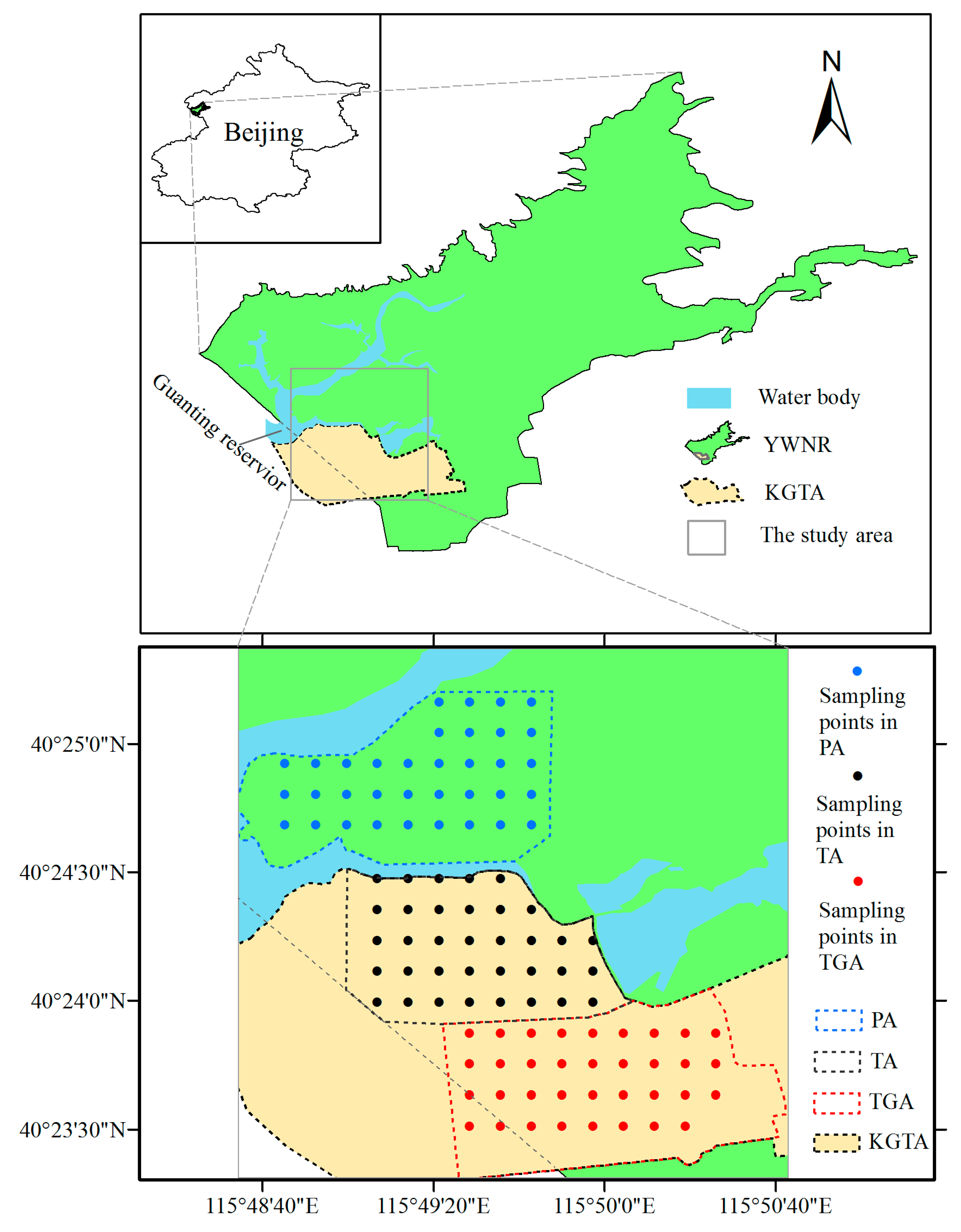
2.1. Study Area

The study sites were located in the Kangxi Grassland Tourist Area (KGTA) and the Yeyahu Wetland Nature Reserve (YWNR) in Yanqing County, Beijing Municipality (115°48′19″–115°49′58″ E, 40°24′29″–40°25′28″ N; see Figure 1). These two areas are located in the fluctuating shore zone of the Guanting Reservoir, which had long been the water source for Beijing City, at least until the excessive use of water upstream of the reservoir for industry and agriculture, combined with deterioration in water quality, caused this to be discontinued [38,39]. Nevertheless, the area around the reservoir is still the largest wetland nature reserve in the Beijing Municipality, with the most diversity of plant and animal species in the region. The main dominant plant species in this area include Phragmites australis, Hemarthria altissima, and Salsola collina, among which Phragmites australis and Hemarthria altissima are the two primary dominant species. This area lies within the north temperate monsoon region, with long, cold winters and hot, rainy summers [40]. The average annual temperature is 9 °C and the average annual rainfall is 436 mm [41].

The local administrative boundary of the YWNR encompasses much of the KGTA (here, the name was given only to distinguish it from the YWNR and to facilitate comparison). However, the relevant administrative authority does not have permission to manage this region. For a long time, the KGTA and YWNR actually belonged to different management institutions with different management objectives [42]. Although the KGTA also has the goal of ecological protection, it permits tourist activities, including hiking and horseback riding, whereas the YWNR is mainly responsible for monitoring and protecting biological diversity, local natural resources, and the environment. Due to its long history of tourism, the KGTA’s plant community composition and structure are significantly different from those of the YWNR, and its soil is usually dry and sandy with less litter on the surface, showing a tendency to decline [43]. In the KGTA, the height of vegetation is usually lower and more uniform, whereas the YWNR has lusher and more diverse vegetation, which provides a better habitat for wild animals such as migratory birds.

2.2. Experimental Design and Sampling

According to their actual management and plant growth situations, we selected three distinct and representative subareas in the study area: a protected area (PA), a trampled area (TA), and a trampled grazed area (TGA) (see Figure 1). The PA has clear management objectives, its own monitoring team, and prohibits any adverse human activity in order to protect the natural environment and biodiversity. In the TA, visitors are permitted to hike or take horseback riding tours on a few designated trails. However, we found that some hikers and riders leave these trails, thereby causing more widespread damage to the vegetation and the wider distribution of horse manure at this site. The TGA is specifically designated for horseback riding and is consequently subject to extensive trampling by horses and tourists and grazing by horses. Horse manure is also widely distributed within this site. There is a clear boundary between the PA and the other two subareas, the TA and the TGA, but there is no such boundary between the two subareas themselves, which we distinguished based on our own field observation and investigation. The two subareas are actually quite different in some respects. The TGA is directly connected to the KGTA entrance and contains almost all its recreational facilities; horses and tourists often gather in this subarea. It is evident that the plant growth here is poor, and the soil quality is worse than that of the adjacent TA. For the convenience of analysis, we artificially created a boundary in the transition zone between these two subareas (see Figure 1). In this study, we regarded PA, TA, and TGA as control, low, and high level of disturbance areas, respectively.

According to our on-site investigation, the number of horses grazing on grassland and providing recreational activities for tourists, such as riding, is approximately 200 and, based on publicly available statistics and our field inquiries, the KGTA attracted 93,000 visitors in 2004, accounting for 0.99% of visitors in the Yanqing District that year [44]. In 2011, 17.37 million tourists visited the district [45], while an estimated 172,000 tourists visited the KGTA based on the above proportion. The KGTA is usually closed in spring and winter every year to prevent fires in the dry season and for maintenance, so visitors are mainly seen in summer and fall.

We conducted field sampling from August to September 2011, a period in which variations in plant growth and community diversity are very small. We sampled 35 systematically placed quadrats (1 m²) in each of the three subareas (see Figure 1). For each quadrat, we recorded the geographical coordinates and took some measurements to characterize the plant communities, including the number of plant species and their respective abundance, average height, coverage, and aboveground biomass (dry matter weight). In addition, the physical and chemical characteristics of the soil in each quadrat were measured, including soil water content, pH, and organic matter. What follows below are the steps that we took. (1) Determination of soil water content. After removing surface floating soil, we used a shovel to obtain a soil sample of about 20 cm depth at a representative point of each quadrat, crushed, removed roots, mixed evenly, and packed it in a marked sealed bag. We brought the fresh soil samples back to the laboratory and immediately placed an appropriate amount in each aluminum box to weigh, then dried them in the oven at 105 °C to a constant weight. We used the electronic balance to weigh and obtain corresponding weight values when the reading was stable. The percentage of lost water in fresh soil samples was calculated as the soil water content of each sample point [46,47]. (2) Determination of soil pH. For each sample, we weighed 10 g of air-dried soil subsample that was passed through a 2 mm sieve and was placed in a 50 mL beaker, with an additional 50 mL of carbon-dioxide-free deionized water; it was stirred vigorously with a glass rod for 1~2 min and we measured the pH value with a pH meter (Professional Meter PP-20, Sartorius Company, Göttingen, Germany) after standing for 30 min. (3) Determination of soil organic matter. We weighed 0.25 g of air-dried soil subsample that passed through 0.25 mm sieve and poured it into the bottom of dry hard glass tube, and then added 5 mL potassium dichromate standard solution and 5 mL concentrated sulfuric acid successively. We heated the hot bath pot (Liquid Paraffin) to 185~190 °C in advance, and put the test tube rack with test tube into the hot oil bath pot for heating. When the solution was boiling in the test tube, the temperature of the bath pot was maintained at 170~180 °C for 5 min. After cooling, we poured the solution in the test tube into a 250 mL triangular flask, added 2~3 drops of o-phenanthroline indicator, and titrated it with 0.2 mol/L FeSO₄ [46,47].

2.3. Data Analysis

We used four diversity indices, including species richness (denoted by R here) [48], Shannon–Wiener (H′) [49,50], evenness (E) [50,51,52], and Simpson index (D) [50,51,53,54] for the measurement of plant diversity. In addition, we used the Jaccard index (J) to assess the degree of similarity between the communities [55]. The specific formulas used for calculating diversity indices and community similarity are as follows (1) to (5). One-way analysis of variance (ANOVA) and Tukey multiple comparisons were used to test the significance of differences in diversity indices and other parameters among the three subareas.

Richness index:

$$\mathrm{R}=\frac{\left(S-1\right)}{lnN}$$

(1)

Shannon-Wiener index:

$${\mathrm{H}}^{\prime }=-{{\displaystyle \sum }}_{i=1}^s{p}_{i}ln{p}_i$$

(2)

Evenness index:

$$\mathrm{E}=\frac{{\mathrm{H}}^{\prime }}{lnS}$$

(3)

Simpson index:

$$\mathrm{D}={{\displaystyle \sum }}_{i=1}^S\frac{n_i\left(n_i-1\right)}{N\left(N-1\right)}$$

(4)

Here, S represents the number of species in the community, N is the total number of individuals, n_i is the number of individuals of the ith species, and p_i is the proportion of the number of individuals of species i in the community.

Jaccard index:

$$\mathrm{J}=\frac{c}{a+b+c}$$

(5)

where c is the number of species that occur in both communities, a indicates the number of species that occur only in community A, and b indicates the number of species that occur only in community B.

The importance value (IV) is a measure for evaluating the dominance of a species within a specific community. It is the mean of its relative coverage, relative density, and relative frequency in a given community [56]. The species with the highest IV is regarded as the dominant species in that community. The relative value of a parameter, such as coverage, refers to the ratio of a species’ coverage to the total plant cover in a community.

We classified species as mesophytic and hygrophytic, according to the relevant literature [57,58] and advice from relevant experts. In addition, we analyzed indicator species by the Indicator Species Analysis program of the Pcord 7.08 (MjM Software Design, Gleneden Beach, OR, USA, 2018).

Maps were drawn using Esri ArcGIS 10.0 software (Esri Inc., Redlands, CA, USA, 1999–2012), and statistical analyses were performed using SPSS 20 (IBM Corp., Armonk, NY, USA, 2011) and Excel 2007 (Microsoft Corp., Redmond, WA, USA, 2006).

3. Results

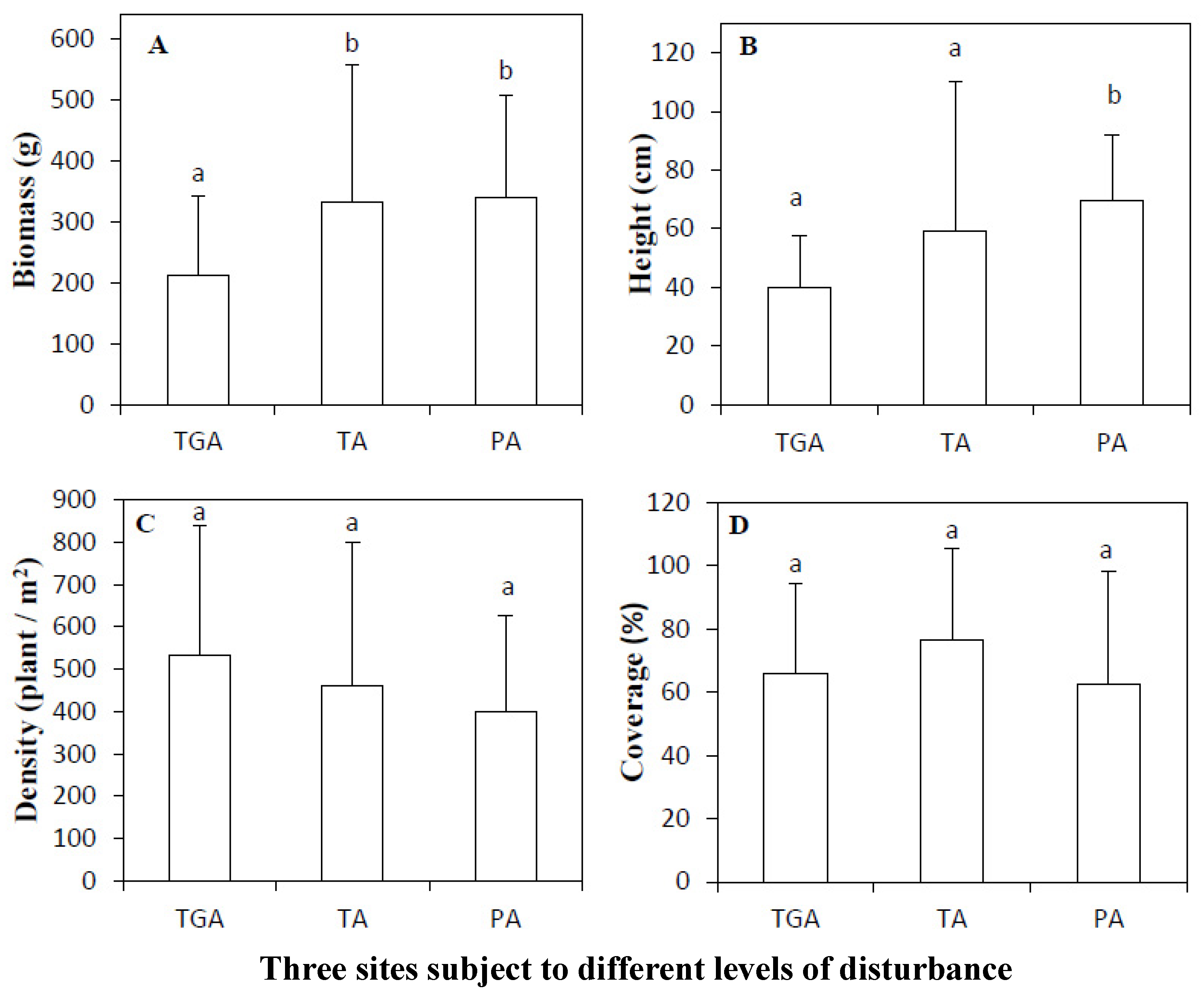
3.1. Comparison of Plant Growth in the Three Subareas

The biomass and average height of plant communities decreased with increasing disturbance, which was highest in the PA, moderate in the TA, and lowest in the TGA. The biomass was significantly lower in the TGA than in the other two subareas, but there was only a significant difference in height between the TGA and the PA (see Figure 2A,B). The density and coverage of plant communities tended to increase with disturbance, although the differences between the subareas were not significant (see Figure 2C,D). Variations in biomass, coverage, and height were the lowest, and the variation in density was lower in the TGA. Except for coverage, which was less variable, variation in the other three parameters was highest in the TA (see Figure 2).

3.2. Composition of Plant Communities and Their Indicators in the Three Subareas

The total number of plant species in the TGA, the TA, and the PA was 36, 49, and 43, respectively. The lowest number of species was found in the TGA and the largest in the TA (see

Table 1. Proportions of mesophytic and hygrophytic plant species at three sites subject to different levels of disturbance in the KGTA and YWNR, Beijing Municipality, China.

Site	N	Mesophytic Species		Hygrophytic Species
		nm (Percentage)	IVm (%)	nh (Percentage)	IVh (%)
TGA	36	28 (77.8%)	53	8 (22.2%)	47
TA	49	37 (75.5%)	49.7	12 (24.5%)	50.3
PA	43	31 (72.1%)	35.7	12 (27.9%)	64.3

N = Total number of species; n_m = number of mesophytic species; n_h = number of hygrophytic species; IV_m = importance value of mesophytic species; IV_h = importance value of hygrophytic species. Numbers in brackets indicate the percentage of the mesophytic or hygrophytic species at each site.

). The most dominant species with the largest IVs in the TA and the PA were Hemarthria altissima (IV of 21.5% in the TA and 36.8% in the PA) and Phragmites australis (IV of 12.2% in the TA and 10% in the PA). In the TGA, Hemarthria altissima was the most dominant species (IV of 32.7%). The next most dominant species was Salsola collina (IV of 10.3%), a mesophytic species that is not preferred by livestock.

The number of mesophytic species accounted for more than 72% of the total number in each subarea. This proportion gradually increased with disturbance, being lowest in the PA and highest in the TGA. The IV of mesophytic species showed the same trend, although these values were not so high. In the TGA, this was just over 50%, and it was lowest in the PA. Mesophytic species were barely dominant in the TGA. However, hygrophytic species were clearly dominant in the PA (see Table 1). In addition, in the dominant species, the IVs of mesophytic species were all less than 50%, whereas the proportion of rare species was far higher than that of dominant species (see

Table 2. Number and importance value (IV) of mesophytic species and their proportion in the dominant (IV > 5%) and rare (IV < 5%) species at three sites subject to different levels of disturbance in the KGTA and YWNR, Beijing Municipality, China.

Site	nm (Percentage)		IVm (%) (Percentage)
	Dominant Species	Rare Species	Dominant Species	Rare Species
TGA	6 (67%)	30 (80%)	77.5 (45%)	22.5 (80%)
TA	6 (50%)	43 (79%)	64.6 (36.8%)	35.4 (75%)
PA	5 (40%)	38 (76%)	62.6 (15.8%)	37.4 (69%)

n_m = number of mesophytic species; IV_m = importance value of mesophytic species. Numbers in brackets indicate the percentage of the number or the important value (IV) of the mesophytic species in the dominant species and the rare species at each site.

). Moreover, the IV of mesophytic species tended to increase with disturbance, being lowest in the PA and highest in the TGA, irrespective of whether these were dominant or rare species, although the trend for rare species was not as obvious as that for the dominant species (see Table 2). In general, the number and proportion of mesophytic species, and especially rare species, are higher in all three subareas. Moreover, more drought-tolerant species have emerged with increasing disturbance.

The indicator species analysis shows that the three subareas have their respective indicator species. The only indicator of the TA is a hygrophytic species, and there are two hygrophytic species among the five indicators of the PA. However, the indicators in the TGA are all mesophytic species (see

Table 3. Indicator species in the three subareas.

TGA	TA	PA
Salsola collina Ixeris chinensis Elymus dahuricus Artemisia scoparia Lespedeza davurica Astragalus adsurgens	Calamagrostis epigejos *	Cynanchum chinensis Inula japonica * Sonchus brachyotus * Artemisia japonica Kummerowia stipulacea

* Hygrophytic plant species.

).

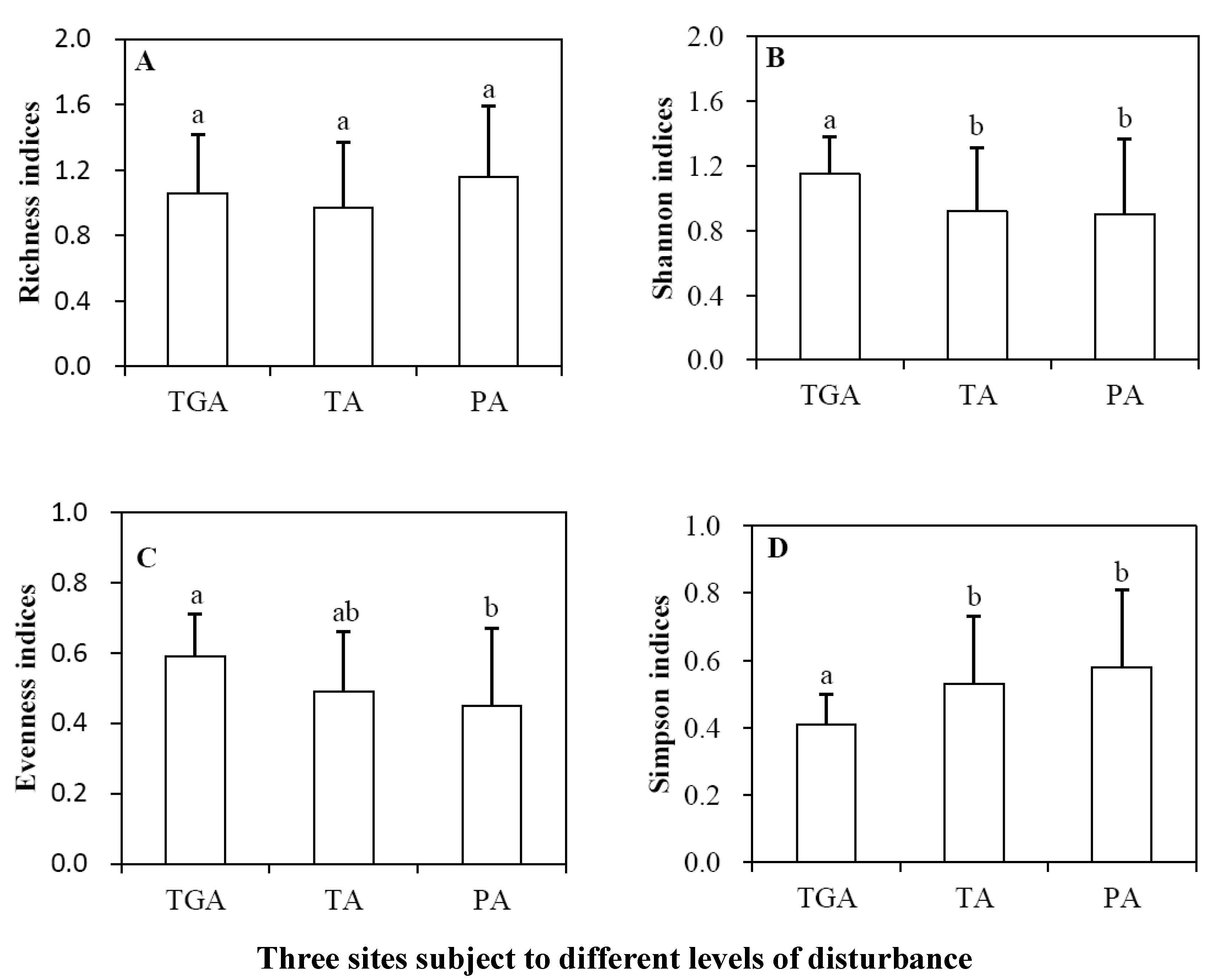
3.3. Plant Diversity of Three Subareas

Species richness was highest in the PA, followed by the TGA and the TA, but these differences were not statistically significant (see Figure 3A). The Shannon and evenness indices generally increased with disturbance, being lowest in the PA and higher in the TA and the TGA (see Figure 3B,C). There were, however, no significant differences in these two indices between the TA and the PA. The Shannon–Wiener index of the TGA was significantly higher than that of the TA and the PA, and the evenness index was only significantly higher than that of the PA. The trend of the Simpson index was the opposite to that of the Shannon and evenness indices (see Figure 3D). This index was significantly lower in the TGA than in the other two subareas, which did not significantly differ from each other in this index.

The standard deviations (SDs) of all four diversity indices were lowest in the TGA (see Figure 3), and SD generally decreased with increasing disturbance. This trend was particularly obvious for the Shannon, evenness, and Simpson indices, but less so for the richness index.

3.4. Community Similarity among Three Subareas

Analysis of community similarity shows that the change in similarity was consistent among the three subareas, irrespective of whether the analysis included all species or just rare species (see

Table 4. Comparison of community similarity among different plant species groups at three sites subject to different levels of disturbance within the KGTA and YWNR, Beijing Municipality, China.

Species Groups	PA and TGA	PA and TA	TGA and TA
Dominant species	0.38	0.38	0.71
Rare species	0.31	0.37	0.46
All species	0.41	0.48	0.55

). The similarity between the PA and the TGA or the TA is lower, whereas that of the two disturbance areas is higher. When the analysis was confined to the dominant species, the similarity between the PA and either of the two disturbance areas is the same. However, the composition of the dominant species showed more similarity in the two disturbed subareas.

3.5. Physical and Chemical Characteristics of the Soil of the Three Subareas

Soil water content tended to decrease with increasing disturbance (see

Table 5. Comparison of physical and chemical characteristics of soil at three sites subject to different levels of disturbance in the KGTA and YWNR, Beijing Municipality, China. Data are means ± standard deviations. Per column, different superscripts indicate statistically significant differences between means (p < 0.05).

Site	Water Content (%)	Organic Matter Content (g/kg)	pH
TGA	4.85 ± 1.69 a	13.97 ± 4.32 a	8.79 ± 0.22 a
TA	10.58 ± 11.56 b	10.67 ± 7.47 b	8.59 ± 0.18 b
PA	13.58 ± 8.72 c	14.22 ± 7.01 a	8.57 ± 0.29 b

) and was significantly lower in the TGA than in the TA and the PA. In the TGA, the soil surface was loose and the deep soil layer was dry and harder, with greater disturbance. In addition, the TGA and the PA had significantly higher soil organic matter content than the TA. Moreover, the soil of the TGA was more alkaline.

The soil water content and organic matter content were least variable in the TGA, and there were no obvious differences in variability in pH among the three subareas (see Table 5).

4. Discussion

4.1. The Rationality of the Division of Subareas

We divided the two disturbed subareas by observing and comparing the on-site recreational facilities, the types and levels of disturbance, and their actual impact. Although there may be some vegetation or environmental similarities near the artificial boundary, and sometimes a few horses cross the boundary of the two subareas, overall, the two subareas are significantly different in the characteristics of plants and soils, as well as the types and levels of disturbance. Certain subjective judgments went into setting the boundary, but that does not affect the purpose of our research, which is to understand the actual state of disturbed plant communities and identify their respective responses and indicators. The results also showed that there were significant differences in plant community composition, diversity, productivity, and soil characteristics between the two subareas (see Figure 2 and Figure 3; see Table 5). Some indicators also showed those differences under disturbance conditions fairly well. Therefore, overall, we found that such a division is both feasible and reasonable, and it could meet our research objectives.

4.2. Responses and Indications of Plant Growth Parameters to Different Levels of Disturbance

In our results, different levels of disturbance have a negative impact on plant biomass and height and, the greater the disturbance, the greater the harm (see Figure 2A,B). Compared with coverage and density, the variations in biomass and height truly reflect the different levels of disturbance experienced in the three subareas, showing a clear indication of these disturbances, especially for areas of severe interference such as the TGA. Our study is similar to some prior studies that focused solely on grazing results [10,13,27,59,60,61], which also showed an adverse effect on productivity. This indicates that parameters, such as biomass, applied to grazing, can also be applied to the assessment of grassland tourism because both grazing and grassland tourism include feeding and trampling on plant communities, and the effects are in some ways similar. Although a certain level of disturbance can significantly reduce productivity, it may also increase plant diversity, such as the Shannon–Wiener index in our study (see Figure 3B). This seems to support the intermediate disturbance hypothesis (IDH), which assumes that species diversity is greatest under a moderate intensity of disturbance [25,26,27,28,62,63]. However, whether this increase in diversity is our true goal needs to be considered in conjunction with the diversity indices used, as well as the productivity and sustainability of the grassland.

Despite the negative impacts of disturbances, individual plants also showed some growth potential. According to our observations, although the aboveground parts of some plants were damaged or destroyed, there was some new seedling growth in other locations, which increased plant density (see Figure 2C). Surviving leaves of damaged plants also tended to increase in size to absorb more sunshine and soil nutrition, which obscured the overall decrease in plant coverage (see Figure 2D).

Not only can the parameters of plant communities indicate their disturbance intensity, but the variation of these parameters can also be used as an important reference for judging the disturbances. For example, SD is usually a measure of data variability around the mean. We can use it indirectly to measure the plant parameters’ spatial variations because each data point represents a certain location in space. In our study, biomass and height and their variations were minimal in the TGA, indicating that different locations of the subarea suffered a similar degree of serious damage. Compared with the TGA, the biomass and height in the TA are higher, and their variation is greater, indicating that the hazard in that subarea is not as severe and extensive as in the TGA.

4.3. Indicator Species in Plant Communities under Different Levels of Disturbance

Grazing and tourism promoted the development of mesophytic species, which are common in this region due to long-term drought conditions [41]. In addition, the proportion of mesophytic species tended to increase with the levels of disturbance (see Table 1). The similarity of species composition between areas gradually reduced with increasing levels of disturbance, and this was even more obvious for dominant species (see Table 4). This is mainly due to the emergence of more mesophytic species, accompanied by an increase in disturbance. In the TGA, the high proportion of mesophytic species is closely related to the significantly lower water content in this subarea (see Table 5), which is due, in part, to grazing and tourism activities. Trampling by livestock and humans and grazing by livestock significantly decreased the height and biomass of plant communities, greatly reduced the accumulation of litter, and degraded the soil, leading to decreased soil water retention and water content. Reduced soil water content is not conducive to the survival of hygrophytic species, which likely explains why mesophytic species have, over years of succession, become dominant in the TGA (see Table 1 and Table 2).

According to the analysis of indicator species, the indicators of the TGA are six mesophyte species, which are actually the plant types that are not palatable to horses. This may be due to the fact that certain characteristics of these plants, such as their unpleasant smell and taste, have made horses avoid them, resulting in their widespread preservation in this area. Our results are similar to those of Pueyoa, Y. et al. [64], which also indicate that some plant species are not palatable to livestock and can act as indicators of heavily grazed areas. There is only one indicator of hygroscopic species in the TA, which indicates that soil moisture in this region is relatively high and plants are less disturbed. There are five indicators in the PA, two of which are hygrophytes, which indicates diverse habitats and plant types. These indicators will provide an important reference and an optional tool for judging the level of disturbance of plant communities in each subarea.

4.4. Indicative Role of Diversity Indices under Different Levels of Disturbance

Grazing and tourism significantly decreased the dominance of plant communities, thereby increasing community evenness and Shannon diversity (see Figure 3B–D). Our results reflect the high level of disturbance throughout the TGA, which can be confirmed from the relatively low variability of vegetation height, biomass, and the three diversity indices measured among sampling points (see Figure 2 and Figure 3). From the perspective of interspecific interactions within plant communities, the larger effect of this disturbance on the dominant species greatly reduced the pressure of interspecific competition for sub-dominant species, including rare species, and indirectly promoted their access to limited resources (e.g., sun, water, and soil nutrients) and their opportunities for growth, thereby increasing the evenness and Shannon diversity of the plant community. This shows that the diversity indices and their variability can indicate the disturbance level of the plant community from different perspectives, particularly for severely disturbed areas. Several studies have also confirmed that grazing disturbance promotes diversity [61], and that diversity was greatest in the presence of moderate disturbance [25,26,27,28,62,63]. However, some of these studies used the Shannon–Wiener index [25,28], while others used the richness index (number of species per unit area) [26,27]. Considering the differences in the environmental background of these studies, the comparison of these results needs to be cautious. Despite similar effects on plant diversity, there are relatively few studies on grazing disturbance combined with tourism.

In cases of natural competition, one or several species in the community tend to occupy a dominant position. Therefore, the dominance is greater, the evenness is lower, and the Shannon–Wiener index is commonly low [61], just as in the case of the PA. In the case of high disturbance areas, such as the TGA, the dominance of plant communities tends to decrease, as does the total number of species, while evenness increases and the Shannon–Wiener index shows an increasing trend. The TA region suffered fewer disturbances and its indices were mostly between the two subareas, but the number of its species was the highest, which indicates that the restraint of disturbance on competition led to the emergence of more species. Therefore, in the case of disturbances, the total number of species may be a better indicator. Dominance, evenness, and the Shannon–Weiner index also better indicate the state of interference. However, the richness index does not show significant differences among the three subareas, and its role as an indicator has certain limitations.

The diversity of plant communities in natural grasslands is an objective reality under specific temporal and spatial conditions. If there is no human interference, the composition and diversity of these communities should be a result of their response to environmental stress and natural succession. It is possible to use diversity indices to measure or compare the characteristics of plant communities. However, using only a diversity index may be misleading because it is difficult to measure the real growth status of plants, the specific species in the community [35], and the sustainability of grassland resources under different levels of disturbance, especially when those levels are high [65]. Although the Shannon and evenness indices of the TGA were high, negative impacts on the vegetation were also apparent in the TGA. For example, the number of total species, productivity (e.g., plant height and biomass), and soil quality were significantly lower in this subarea than the less disturbed subareas. In addition, more drought-tolerant species occurred in this subarea. Thus, despite its relatively high Shannon and evenness indices, plant communities in the TGA have actually been severely adversely affected by disturbance. If we only observe and compare diversity indices without considering the types and intensity of the disturbances and actual plant growth, we may reach inaccurate conclusions, which misinform protection and management policies. Therefore, to accurately grasp the productivity and sustainability of grassland resources, we need to understand not only the plant diversity of the grasslands but also the health of said plants.

4.5. Indicators of Soil Characteristics under Different Levels of Disturbance

Soil water content is a good indicator of different disturbances [66]. In the TGA, sustained high grazing intensity and tourist activity reduced plant height, loosened the soil surface, and hardened the soil, none of which are conducive to moisture retention. The thin layer of branches and leaves and the lack of litter in this subarea make it relatively easy for any soil water that is present to evaporate. These are the main causes of the significant decrease in soil water content in this subarea (see Table 5). The reduction in litter accompanied by disturbance and the resulting decrease in soil water content has also been confirmed by two other studies [67,68]. The other two subareas have a higher soil water content, which is closely related to more successful vegetation growth (such as height and coverage) and less disturbance in these two regions.

Organic matter content can also indicate different disturbance levels. As organic matter can be converted into nutrients for plant growth, the amount of organic matter can be regarded as an indicator of soil fertility. For example, in the PA, the organic matter content is high, the soil is relatively fertile, and the plant grows better. However, in the two disturbed areas, the TA and the TGA, the distribution and quantity of horse droppings are different due to the different degrees of disturbance. Accordingly, these are inevitably reflected in the content of soil organic matter in these two areas (see Table 5). Therefore, the organic matter content also indicates the disturbance level in different regions. Although there was no difference in the amount of organic matter between the TGA and the PA, the main sources of organic matter differed between these subareas. The PA’s organic matter was mainly due to its higher plant biomass and thicker litter layer, whereas the TGA’s was mainly comprised of horse droppings rather than biomass or litter. This result is consistent with that of Walters and Martin [59] but contrary to that of Pei et al. [60]. This discrepancy is likely the result of the combined effects of feeding and excretion of livestock on soil nutrition under different grazing intensities. In our study, horse droppings have become an important component of organic matter in the TGA due to the sharp reduction in litter caused by grazing in that area. This suggests that the soil fertility of grazed areas can be maintained, or at least not be reduced. However, in the TGA, the lower soil water content, higher soil alkalinity, and desertification are extremely disadvantageous for the effective utilization of the soil’s nutrients by plants and the maintenance of the soil’s fertility, and are, therefore, not conducive to plant growth and development. The soil quality in the TGA is clearly declining. The TA has been plowed and planted with alfalfa for livestock feed. In addition, it has less horse manure than the TGA and, consequently, less accumulated organic matter than the other two subareas.

4.6. Management Applications

(1) In a broad sense, indicators, including those of plant communities, provide an optional and convenient tool for monitoring the levels of disturbance in the grassland plant community. We can easily observe and judge the site’s conditions by observing indicators such as the height and coverage of plants, the condition of plants being eaten and trampled, other interference factors such as the number of tourists and the paths they travel, the distribution of amusement facilities, the feeding area and quantity of horses, and the quantity and distribution of horse manure. In addition, a quick judgment can be made by the type and distribution of the indicator species. For example, the occurrence and frequency of mesophyte and grazing-tolerance species can be used to judge the damaged status of plants.

On the basis of field observation, the level of disturbance of the plant community needs to be further evaluated through investigation and comprehensive analysis of plant composition, diversity, and soil conditions. For example, the level of disturbance of plant communities or the health of these communities can be judged comprehensively by multiple diversity indexes, combined with the average height and biomass of the community, proportion of mesophytes, as well as soil hardness and humidity.

(2) The lack of effective management is a crucial factor that has led to the current situation. It is necessary to develop an effective monitoring system and put this into practice [1,69]. In addition, management activities should be scientific and reasonable [1,7,8]. For example, a reasonable livestock carrying capacity and visitor numbers should be determined according to the available grassland resources. In order to reduce human interference as much as possible, there is a need to strengthen the guidance and supervision of human activity [1,2,7].

(3) Restoration of degraded grassland areas is required. One method of restoration could be rotational grazing, or even fencing in, of some less degraded areas [1,16]. This has been shown to be an effective method for restoring and managing grasslands [61,70]. Artificial restoration is required to restore the ecological function of severely degraded grasslands. Through these measures, we may be able to maintain a dynamic balance between maintaining productivity, biodiversity, and tourism.

5. Conclusions

The results of this study confirm our hypotheses. The density and coverage of the plant community have a certain compensatory increase under disturbance conditions. With the increase in disturbances, more drought-tolerant species have appeared, some of which have become the grazing-tolerance indicator species in the TGA. For plant community productivity, biomass and height are good indicators for distinguishing different disturbances. In addition, several diversity indices indicate the change of plant communities from different perspectives. For soil parameters, soil water content and organic matter concentration help to indicate different disturbance levels. The SD of the plant community and soil parameters is also a good indicator of their spatial variability and levels of disturbance, especially for the TGA. Our analysis confirms that the indicators of productivity, diversity, and soil parameters all reveal the disturbance level in each subarea from different angles. However, under disturbed conditions, a more comprehensive analysis of these indicators is needed before we can accurately understand the health of the plant community.

References

1. Zhong, L.-S.; Niu, Y.-F.; Liu, J.-M.; Chen, T. Development of Grassland Tourism Resource in Inner Mongolia Autonomous Region. J. Arid Land Resour. Environ. 2005, 19, 105–110. [Google Scholar]
2. Shi, K.-B.; Wang, W.-R.; Yang, Y.-C.; Shao, R.; Shi, Y.-B. Impacts of tourists’activities on vegetation of Gannan grassland—A case study on tourist spot of Sangke prairie. Arid Zone Res. 2015, 32, 1220–1228. [Google Scholar]
3. Mainguet, M. Desertification: Natural Background and Human Mismanagement; Speringer: Berlin/Heidelberg, Germany, 1994. [Google Scholar]
4. Manzano, M.G.; Návar, J. Processes of desertification by goats overgrazing in the Tamaulipan thornscrub (matorral) in north-eastern Mexico. J. Arid Environ. 2000, 44, 1–17. [Google Scholar] [CrossRef]
5. Su, Y.-Z.; Li, Y.-L.; Cui, J.-Y.; Zhao, W.-Z. Influences of continuous grazing and livestock exclusion on soil properties in a degraded sandy grassland, Inner Mongolia, northern China. Catena 2005, 59, 267–278. [Google Scholar] [CrossRef]
6. Liu, L.-M.; Lv, J. The environmental influence of tourism on vegetation in typical grassland areas. Resour. Sci. 2009, 31, 442–449. [Google Scholar]
7. Gao, X.-M.; Ma, K.-P.; Chen, L.-Z.; Li, D.-Q. The effects of tourism on species diversity of subalpine meadows in Dongling mountainous area, Beijing. Biodivers. Sci. 2002, 10, 189–195. [Google Scholar]
8. Wu, J.-Z.; Shangguan, T.-L.; Zhang, J.; Li, J.-C.; Cao, T.-W.; Yue, J.-Y. Disturbing effects of tourism on plant species diversity of Malun subalpine meadow, Shanxi Province. J. MT Sci. 2007, 25, 534–540. [Google Scholar]
9. Turner, C.L.; Seastedt, T.R.; Dyer, M.I. Maximization of aboveground grassland production—The role of defoliation frequency, intensity, and history. Ecol. Appl. 1993, 3, 175–186. [Google Scholar] [CrossRef]
10. Virtanen, R. Effects of Grazing on Above-Ground Biomass on a Mountain Snowbed, NW Finland. Oikos 2000, 90, 295–300. [Google Scholar] [CrossRef]
11. Patton, B.D.; Dong, X.J.; Nyren, P.E.; Nyren, A. Effects of Grazing Intensity, Precipitation, and Temperature on Forage Production. Rangel. Ecol. Manag. 2007, 60, 656–665. [Google Scholar] [CrossRef]
12. de Mazancourt, C.; Loreau, M.; Abbadie, L. Grazing Optimization and Nutrient Cycling: When Do Herbivores Enhance Plant Production? Ecology 1998, 79, 2242–2252. [Google Scholar] [CrossRef]
13. Semmartin, M.; Oesterheld, M. Effects of grazing pattern and nitrogen availability on primary productivity. Oecologia 2001, 126, 225–230. [Google Scholar] [CrossRef]
14. Li, C.; Hao, X.; Zhao, M.; Han, G.; Willms, W.D. Influence of historic sheep grazing on vegetation and soil properties of a Desert Steppe in Inner Mongolia. Agric. Ecosyst. Environ. 2008, 128, 109–116. [Google Scholar] [CrossRef]
15. Fedorov, N.I.; Zharkikh, T.L.; Mikhailenko, O.I.; Bakirova, R.T.; Martynenko, V.B. Forecast changes in the productivity of plant communities in the pre-urals steppe site of orenburg state nature reserve (russia) in extreme drought conditions using ndvi. Nat. Conserv. Res. 2019, 4 (Suppl. 2), 104–110. [Google Scholar] [CrossRef]
16. Bulgakova, M.A.; Pyatina, E.V. The role of ungulates in soil zoocoenosis development of the steppe zone of the urals. Nat. Conserv. Res. 2019, 4 (Suppl. 2), 94–97. [Google Scholar] [CrossRef]
17. Biondini, M.E.; Patton, B.D.; Nyren, P.E. Grazing Intensity and Ecosystem Processes in a Northern Mixed-Grass Prairie, USA. Ecol. Appl. 1998, 8, 469–479. [Google Scholar] [CrossRef]
18. Hickman, K.R.; Hartnett, D.C.; Cochran, R.C.; Owensby, C.E. Grazing management effects on plant species diversity in tallgrass prairie. J. Range Manag. 2004, 57, 58–65. [Google Scholar] [CrossRef]
19. Battisti, C.; Poeta, G.; Fanelli, G. An Introduction to Disturbance Ecology; Springer International Publishing: Cham, Switzerland, 2016. [Google Scholar]
20. Waser, N.M.; Price, M.V. Effects of Grazing on Diversity of Annual Plants in the Sonoran Desert. Oecologia 1981, 50, 407–411. [Google Scholar] [CrossRef]
21. Pykälä, J. Cattle Grazing Increases Plant Species Richness of Most Species Trait Groups in Mesic Semi-Natural Grasslands. Plant Ecol. 2004, 175, 217–226. [Google Scholar] [CrossRef]
22. Marty, J.T. Effects of Cattle Grazing on Diversity in Ephemeral Wetlands. Conserv. Biol. 2005, 19, 1626–1632. [Google Scholar] [CrossRef]
23. Schultz, N.L.; Morgan, J.W.; Lunt, I.D. Effects of grazing exclusion on plant species richness and phytomass accumulation vary across a regional productivity gradient. J. Veg. Sci. 2011, 22, 130–142. [Google Scholar] [CrossRef]
24. Shi, X.-M.; Li, X.G.; Li, C.T.; Zhao, Y.; Shang, Z.H.; Ma, Q. Grazing exclusion decreases soil organic C storage at an alpine grassland of the Qinghai–Tibetan Plateau. Ecol. Eng. 2013, 57, 183–187. [Google Scholar] [CrossRef]
25. Sasaki, T.; Okubo, S.; Okayasu, T.; Jamsran, U.; Ohkuko, T.; Takeuchi, K. Management Applicability of the Intermediate Disturbance Hypothesis across Mongolian Rangeland Ecosystems. Ecol. Appl. 2009, 19, 423–432. [Google Scholar] [CrossRef] [Green Version]
26. Fensham, R.J.; Silcock, J.L.; Dwyer, J.M. Plant species richness responses to grazing protection and degradation history in a low productivity landscape. J. Veg. Sci. 2011, 22, 997–1008. [Google Scholar] [CrossRef]
27. Deng, L.; Sweeney, S.; Shangguan, Z.P. Grassland responses to grazing disturbance: Plant diversity changes with grazing intensity in a desert steppe. Grass Forage Sci. 2014, 69, 524–533. [Google Scholar] [CrossRef]
28. Ganjurjav, H.; Duan, M.-J.; Wan, Y.-F.; Zhang, W.-N.; Gao, Q.-Z.; Li, Y.; Jiangcun, W.-Z.; Danjiu, L.-B.; Guo, H.-B. Effects of grazing by large herbivores on plant diversity and productivity of semi-arid alpine steppe on the Qinghai-Tibetan Plateau. Rangel. J. 2015, 37. [Google Scholar] [CrossRef]
29. Proulx, M.; Mazumder, A. reversal of grazing impact on plant species richness innutrient-poor vs. nutrient-rich ecosystems. Ecology 1998, 79, 2581–2592. [Google Scholar] [CrossRef]
30. Osem, Y.; Perevolotsky, A.; Kigel, J. Grazing Effect on Diversity of Annual Plant Communities in a Semi-Arid Rangeland: Interactions with Small-Scale Spatial and Temporal Variation in Primary Productivity. J. Ecol. 2002, 90, 936–946. [Google Scholar] [CrossRef]
31. Shrestha, G.; Stahl, P.D. Carbon accumulation and storage in semi-arid sagebrush steppe: Effects of long-term grazing exclusion. Agric. Ecosyst. Environ. 2008, 125, 173–181. [Google Scholar] [CrossRef]
32. Austrheim, G.; Eriksson, O. Plant Species Diversity and Grazing in the Scandinavian Mountains: Patterns and Processes at Different Spatial Scales. Ecography 2001, 24, 683–695. [Google Scholar] [CrossRef]
33. Fernández-Lugo, S.; de Nascimento, L.; Mellado, M.; Arévalo, J.R. Grazing effects on species richness depends on scale: A 5-year study in tenerife pastures (canary islands). Plant Ecol. 2011, 212, 423–432. [Google Scholar] [CrossRef]
34. Jing, Z.; Cheng, J.; Su, J.; Bai, Y.; Jin, J. Changes in plant community composition and soil properties under 3-decade grazing exclusion in semiarid grassland. Ecol. Eng. 2014, 64, 171–178. [Google Scholar] [CrossRef]
35. O’Connor, T.G.; Martindale, G.; Morris, C.D.; Short, A.; Witkowski, E.T.F.; Scott-Shaw, R. Influence of Grazing Management on Plant Diversity of Highland Sourveld Grassland, KwaZulu-Natal, South Africa. Rangel. Ecol. Manag. 2011, 64, 196–207. [Google Scholar] [CrossRef]
36. Fenu, G.; Cogoni, D.; Ulian, T.; Bacchetta, G. The impact of human trampling on a threatened coastal Mediterranean plant: The case of Anchusa littorea Moris (Boraginaceae). Flora Morphol. Distrib. Funct. Ecol. Plants 2013, 208, 104–110. [Google Scholar] [CrossRef]
37. Santoro, R.; Jucker, T.; Prisco, I.; Carboni, M.; Battisti, C.; Acosta, A.T.R. Effects of Trampling Limitation on Coastal Dune Plant Communities. Environ. Manag. 2012, 49, 534–542. [Google Scholar] [CrossRef]
38. Du, G.-S. The study of trophic condition of Kwangting reservoir. J. Teach. Coll. (Nat. Sci. E) 1989, 10, 56–61. [Google Scholar]
39. Du, G.S.; Wang, J.T.; Zhang, W.H.; Feng, L.Q.; Liu, J. On the nutrient status of guanting reservoir, 2001–2002. J. Lake Sci. 2004, 16, 277–281. [Google Scholar]
40. Zhao-Ning, G.; Gong, H.-L.; Zhao, W.-J. The Ecological Evolution of Beijing Wetland: A Case Study in Beijing Wild Duck Lake; Beijing Science &Technology Press: Beijing, China, 2007. [Google Scholar]
41. Wang, Z.; Gong, H.; Zhang, J. Receding water line and interspecific competition determines plant community composition and diversity in wetlands in Beijing. PLoS ONE 2015, 10, e0124156. [Google Scholar] [CrossRef]
42. Zhao, W.J.; Wang, Y.H.; Gong, Z.N.; Hu, D.Y. 3S Integrated Practice Instruction-Taking Yeyahu Wetland as an Example; China Environmental Science Press: Beijing, China, 2011. [Google Scholar]
43. Wang, Y.; Gong, H.L.; Zhao, W.J.; Li, X.J.; Zhang, Z.F.; Zhao, W. The change of Yeyahu wetland resources in Beijing. Acta Geogr. Sin. 2005, 60, 656–664. [Google Scholar]
44. Beijing Municipal Bureau of Statistics. Statistical Bulletin of the National Economic and Social Development of Yanqing County, Beijing. 2004. Available online: http://www.tjcn.org/tjgb/01bj/247.html (accessed on 5 October 2020).
45. Bureau of Statistics of Yanqing County, Beijing. Statistical Bulletin of the National Economic and Social Development of Yanqing County, Beijing. 2011. Available online: http://www.tjcn.org/tjgb/01bj/25878_2.html (accessed on 5 October 2020).
46. Xie, X.M. Soil and Plant Nutrition Experiment; Zhejiang University Press: Hangzhou, China, 2014. [Google Scholar]
47. Bao, S.D. Soil and Agricultural Chemistry Analysis; China Agricultural Press: Beijing, China, 2000. [Google Scholar]
48. Clifford, H.T.; Stephenson, W. An Introduction to Numerical Classification; Academic Press: London, UK, 1975. [Google Scholar]
49. Shannon, C.E.; Weaver, W. The Mathematical Theory of Communication; University of Illinois Press: Urbana, IL, USA, 1949. [Google Scholar]
50. Magurran, A.E. Measuring Biological Diversity; Blackwell Publishing Company: Malden, MA, USA, 2004. [Google Scholar]
51. Pielou, E.C. An Introduction to Mathematical Ecology; Wiley InterScience: New York, NY, USA, 1969. [Google Scholar]
52. Pielou, E.C. Ecological Diversity; Wiley InterScience: New York, NY, USA, 1975. [Google Scholar]
53. Simpson, E.H. Measurement of diversity. Nature 1949, 163, 688. [Google Scholar] [CrossRef]
54. Magurran, A.E. Ecological Diversity and Its Measurement; Princeton University Press: Princeton, NJ, USA, 1988. [Google Scholar]
55. Krebs, C.J. Ecological Methodology; Benjamin/Cummings: Menlo Park, CA, USA, 1999. [Google Scholar]
56. Wang, B. Phytocoenology; Higher Education Press: Beijing, China, 1987. [Google Scholar]
57. Chen, W.; Hu, D.; Fu, B.Q. Research on Biodiversity in Beijing Wetland; Science Press: Beijing, China, 2007. [Google Scholar]
58. Gong, Z.N.; Gong, H.L.; Hu, D. Wetlnd Plants in Wild Duke Lake, Beijing; China Environmental Science Press: Beijing, China, 2012. [Google Scholar]
59. Walters, C.M.; Martin, M.C. An Examination of the Effects of Grazing on Vegetative and Soil Parameters in the tallgrass praire. Trans. Kans. Acad. Sci. 2003, 106, 59–70. [Google Scholar] [CrossRef]
60. Pei, S.; Fu, H.; Wan, C. Changes in soil properties and vegetation following exclosure and grazing in degraded Alxa desert steppe of Inner Mongolia, China. Agric. Ecosyst. Environ. 2008, 124, 33–39. [Google Scholar] [CrossRef]
61. Wu, G.L.; Du, G.Z.; Liu, Z.H.; Thirgood, S. Effect of fencing and grazing on a kobresia-dominated meadow in the qinghai-tibetan plateau. Plant Soil 2009, 319, 115–126. [Google Scholar] [CrossRef]
62. Gao, J.J.; Carmel, Y. Can the intermediate disturbance hypothesis explain grazing–diversity relations at a global scale? Oikos 2020, 129, 493–502. [Google Scholar] [CrossRef]
63. Li, J.; Loneragan, W.A.; Duggin, J.A.; Grant, C.D. Issues affecting the measurement of disturbance response patterns in herbaceous vegetation—A test of the intermediate disturbance hypothesis. Plant Ecol. 2004, 172, 11–26. [Google Scholar] [CrossRef]
64. Pueyoa, Y.; Aladosa, C.L.; Ferrer-Benimelib, C. Is the analysis of plant community structure better than common species-diversity indices for assessing the effects of livestock grazing on a Mediterranean arid ecosystem? J. Arid Environ. 2006, 64, 698–712. [Google Scholar] [CrossRef]
65. Battisti, C.; Contoli, L. Diversity Indices as ‘Magic’ Tools inLandscape Planning: A Cautionary Note on their Uncritical Use. Landsc. Res. 2011, 36, 111–117. [Google Scholar] [CrossRef]
66. Weber, K.T.; Gokhale, B.S. Effect of grazing on soil-water content in semiarid rangelands of southeast Idaho. J. Arid Environ. 2011, 75, 464–470. [Google Scholar] [CrossRef]
67. Willms, W.D.; McGinn, S.M.; Dormaar, J.F. Influence of litter on herbage production in the mixed prairie. J. Range Manag. 1993, 46, 320–324. [Google Scholar] [CrossRef] [Green Version]
68. Snyman, H.A. Root studies on grass species in a semi-arid South Africa along a degradation gradient. Agric. Ecosyst. Environ. 2009, 130, 100–108. [Google Scholar] [CrossRef]
69. Battisti, C.; Amori, G.; Luiselli, L. Toward a new generation of effective problem solvers and project-oriented applied ecologists. Web Ecol. 2020, 20, 11–17. [Google Scholar] [CrossRef]
70. Wu, G.-L.; Liu, Z.-H.; Zhang, L.; Chen, J.-M.; Hu, T.-M. Long-term fencing improved soil properties and soil organic carbon storage in an alpine swamp meadow of western China. Plant Soil 2010, 332, 331–337. [Google Scholar] [CrossRef]
Figure 1. Location of the study area and sampling points within subareas subject to three management regimes in the Kangxi Grassland Tourist Area (KGTA) and the Yeyahu Wetland Nature Reserve (YWNR) in the Beijing Municipality. The trampled grazed area (TGA) is shown within the red dotted line. The trampled area (TA) is shown within the black dotted line. The protected area (PA) is shown within the blue dotted line. The diagonal dashed line indicates the boundary of YWNR within the KGTA.
Diversity 13 00252 g001
Figure 2. Variation (standard deviation) in biomass (A), height (B), density (C), and coverage (D) of plant communities at three sites subject to different levels of disturbance in the KGTA and YWNR, Beijing Municipality, China. Height of bars indicates mean values, and length of error bars indicates standard deviation. Per parameter, different letters indicate statistically significant differences between means (p < 0.05).
Diversity 13 00252 g002
Figure 3. Comparison of the means of four diversity indices: richness (A), Shannon (B), evenness (C), and Simpson (D), and their standard deviations (error bars) at three sites subject to different levels of disturbance in the KGTA and YWNR, Beijing Municipality, China. Per diversity index, different superscripts indicate statistically significant differences between means (p < 0.05).
Diversity 13 00252 g003