Article

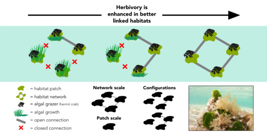
Being Well-Connected Pays in a Disturbed World: Enhanced Herbivory in Better-Linked Habitats

1
Australian Rivers Institute-Coast & Estuaries, School of Environment & Science, Griffith University, Gold Coast, Queensland 4222, Australia
2
Australian Rivers Institute-Coast & Estuaries, School of Environment & Science, Griffith University, Nathan, Queensland 4111, Australia
3
School of Science & Engineering, University of the Sunshine Coast, Maroochydore DC, Queensland 4558, Australia
*
Author to whom correspondence should be addressed.
Diversity 2020, 12(11), 424; https://doi.org/10.3390/d12110424
Submission received: 13 October 2020 / Revised: 2 November 2020 / Accepted: 10 November 2020 / Published: 12 November 2020
(This article belongs to the Section Marine Diversity)

Abstract

:
Seascapes are typically comprised of multiple components that are functionally linked by the movement of organisms and fluxes of matter. Changes to the number and spatial arrangement of these linkages affect biological connectivity that, in turn, can alter ecological functions. Herbivory is one such function, pivotal in controlling excessive algal growth when systems become disturbed. Here, we used microcosm experiments to test how the change to connectivity affects herbivory under different levels of disturbance. We applied network theory to measure types of connectivity at different scales (patch and whole system) and quantified herbivory by a crustacean mesograzer exposed to excess algae, mimicking pulse and press disturbances. We demonstrate that greater connectivity significantly enhances herbivory in Clibanarius virescens: Both the number of linkages and their spatial arrangement interact to shape the response of herbivory in systems to disturbance. Our findings highlight the value of controlled experiments for advancing theories about the potential effects of connectivity on important ecological functions, such as herbivory, and justify further investigation to measure how connectivity might affect the resilience of ecosystems. We posit that the variation in the type, and scale, of spatial linkages might have profound consequences for managing the capacity of ecosystems to respond to disturbance.

Graphical Abstract

1. Introduction

The movements of organisms, nutrients and energy connect populations and ecosystems [1,2]. Connectivity can influence the composition and diversity of assemblages, especially those responding to disturbance [3,4,5]. As a result, connectivity can also affect the distribution and efficacy of important ecological functions, such as herbivory, predation, scavenging and the dispersal of seeds, larvae and pollen [6,7,8,9,10,11,12]. Spatial linkages can also alter how ecosystems respond to disturbance by modifying key functions that underpin the capacity for resilience [13,14,15]. For example, the spatial configuration of wildlife corridors on land, and marine reserve networks in the sea, can influence dispersal patterns, modify the diversity of responses by individuals contributing to the same ecosystem function and determine the potential for ecosystems to recover from disturbance [6,16,17].
Herbivory is an important process in aquatic systems that confers resilience in the face of a disturbance by helping ecosystems to resist shifts to alternative states [3,18,19]. The relationship between herbivory and coral reef resilience is particularly well-understood; examples include: (i) Herbivores in lagoons prevent the overgrowth of corals by macro-algae [3]; (ii) roving herbivores influence the rate of grazing over depth gradients [20]; and (iii) coral reef resilience can be at risk even under low levels of fishing pressure on herbivorous fish [21]. Examples from habitats such as rocky reefs and seagrass meadows also demonstrate the critical role that herbivores play in controlling the growth of algae [22,23,24], a key process necessary for resilient ecosystems. Ensuring that important ecological functions, such as herbivory, are maintained in the face of disturbances is, therefore, important for managers of ecosystems that rely on such functions.
There is evidence to suggest that connectivity influences ecological functions [25]. Field studies have documented this effect with empirical data. For example, the connectivity of larval populations affects the resilience of algal-dominated coral reefs [14], and grazing by fish that use reefs can prevent disturbed reefs from shifting to an algal-dominated state [3]. Directly measuring and testing connectivity in the field can, however, be very difficult because ecological systems are comprised both of numerous different habitat types and a diversity of distinct habitat patches. These components are potentially linked by biological connections that operate at different scales [26,27]. Controlled experiments are an effective alternative to field experiments and can help advance theories about how ecosystem functions are linked to connectivity [28,29,30,31].
Here, we test the effect of changes in connectivity on an important ecosystem function in two microcosm experiments. The experiments were designed to measure how different levels of connectivity shape the response of a key ecological process, grazing of algae (herbivory), to a disturbance event (simulated algal bloom). The microcosms comprised multiple distinct patches and we varied the level of connectivity among patches using different spatial configurations of connections between patches (by varying both the number and location (configuration) of connections). We applied a spatially distinct disturbance event to part of the system (excess algal growth mimicking blooms that occur in eutrophic waters) and measured herbivory responses to press- and pulse-style disturbances in two separate experiments. We hypothesised that (i) patches with greater connectivity would have greater rates of herbivory, because they are more accessible to grazers, (ii) increases in connectivity across a whole system would increase herbivory, (iii) how the connections were configured would influence herbivory, and (iv) the influence of configuration on herbivory would be more visible during a press disturbance.

2. Materials and Methods

We tested the effect of connectivity on herbivory by placing mesograzers (yellow-footed hermit crabs, Clibanarius virescens) into microcosms with different spatial configurations of patches. We then measured herbivory rates under two disturbance scenarios and under seven different types of connectivity between patches. We selected the yellow-footed hermit crab as our model species because it is commonly found on intertidal and subtidal reefs in tropical to warm-temperate regions in the Indo-Pacific region, with demonstrated evidence that disturbances affect their grazing performance [32]. Disturbance in the current study was in the form of excess algal pellets added to specific patches within the system. This disturbance represents a scenario where, for example, parts of an embayment close to major nutrient inputs (e.g., estuarine plumes, sewage or storm-water effluent) are affected by algal blooms [33,34], whereas adjacent areas are not substantially altered by excess algae (for example, Yabsley et al. [35]).

2.1. System Design

We created microcosms with different features to test how connectivity affects mesograzer consumption under conditions that mimic systems partially affected by algal blooms. Microcosms were constructed with nine equally sized patches (patch size: 12 × 12 cm; system size: 36 × 36 cm), arranged in a square, and divided by white acrylic sheets (3 mm thick, 5 cm high; see Figure S1 for an example system). System connectivity was manipulated by varying the number and location of connections between patches; connections were openings in the wall (3 × 3 cm) that allowed the animals to move directly between adjacent patches. We added excess algal pellets to certain patches within the microcosm, mimicking algal bloom conditions in a disturbed system but leaving part of the system in an undisturbed state (Figure 1). The system was spatially configured so that all disturbed patches were connected to each other, whereas the spatial arrangement of connections between the undisturbed and disturbed parts varied among systems (Figure 1).
By changing the number of connections and the way they were configured between undisturbed and disturbed patches (Figure 1), we were able to use two connectivity metrics at both the patch and whole-of-system scales (see Appendix A), and we used network theory to quantify connectivity. Network theory, a form of graph theory, is used to quantify connectivity in a wide variety of systems, including social systems [36], communication and transport systems [37], and ecosystems [38,39]. Metrics have been used to index multiple aspects of connectivity, ranging from simple measures such as the number of connections directly linking a single patch, to integrated measures of connections across the entire spatial configuration of a system [27,40]. The metric of closeness centrality is the inverse of the sum of the shortest path lengths between a node of interest and all other nodes in the system [36]. Closeness centrality provides a useful description of the patterns of connectivity likely to be found in the field [41].
Using multiple metrics to analyse the connectivity of a system or habitat patch can provide detailed information to assist in the management of anthropogenic impacts on connectivity [27]. The first metric of connectivity used in our experiments at the patch scale was the number of connections that linked disturbed patches to neighbouring patches (Table 1; Appendix A). At the system scale, the first metric of connectivity was the number of connections linking the undisturbed to the disturbed part, yielding four possible configurations (Figure 1, Figure A1). Next, we created alternative configurations of connections between the undisturbed and disturbed part of the systems, excluding arrangements that mirrored each other, while keeping to a practical number of systems amenable for testing, and this resulted in a total of seven systems (Figure 1, Appendix A). We quantified the configuration using the network theory metric, closeness centrality [36] for each disturbed patch and at the whole-of-system scale (see Appendix A for details on how these metrics were calculated for our experimental systems). The configuration metric resulted in values ranging between 3.4 and 8.3 for patch-scale and between 18.1 and 58.3 for system-scale, where patches or systems with lower values are less connected than those with higher values (Table 1; Appendix A). Closeness centrality accounts for the topographical distance between patches of interest; thus, our metric for configuration accounted for the placement of the patches and the different distances that the animals needed to move to reach the patches with excess algae. For example, patch B (Table 1) does not have any direct connections from undisturbed patches and the consistently lower values for configuration reflect this; however, in one situation (model system one), patch D is more isolated than patch B and, thus, patch D has a lower value for configuration.
Crabs of approximately the same size were collected from Burleigh Heads, Australia, in May 2016. Crabs were acclimatised in a controlled-temperature laboratory at Griffith University on the Gold Coast, Australia, to the following average conditions: Temperature 24.8 °C, salinity 35.5 ppt, pH 7.8, 12 h night-day cycle from 6 am to 6 pm. Crabs were housed together to allow the opportunity for interactions, limiting the likelihood of behaviour changes in response to unfamiliar individuals being a factor during experiments. Crabs were fed every four days on the same algal pellets used during experiments (New Life Spectrum Marine Fish Formula, 1 mm sinking pellets). Experiments were conducted on scheduled feeding days during June 2016 between 08:00 and 16:00 (hours where crabs were observed to be active) inside the same controlled-temperature laboratory where they were housed. Individuals for experiments were randomly selected from aquaria prior to feeding on scheduled feeding days (individuals observed to be moulting, carrying eggs or have moved to a larger shell were excluded from experiments to account for any behaviour or size change that might affect their consumption). The model systems were placed into separate containers and filled with filtered sea water collected from the Gold Coast seaway to 4 cm (more than enough for all crabs to be fully submerged) under the same conditions (temperature/salinity/pH) they were acclimatised to. One crab was placed into each of the nine patches. We measured the rates (number of pellets h−1 ind−1) at which crabs consumed algal pellets (mean = 2.7, SE 0.1) in pilot studies (n = 10 trials), to ensure that consumers had the capacity to measurably influence the number of algal pellets introduced.

2.2. Press Versus Pulse Herbivory Experiments

We applied two different styles of disturbance (separately) to the microcosms to test whether responses to press-style disturbances were different to pulse disturbances. In both experiments, each of the seven systems were replicated six times, yielding 42 measurements for system-level analyses and 168 observations for patch-level analyses. A summary of the length of the experiment and distribution of algal pellets can be found in Table 2.
In both the press and pulse disturbance experiments, one algal pellet was added to undisturbed patches because it is less than the normal consumption of a single crab (3 pellets h−1 expected under optimal conditions [32]). In an analogous field situation, this represents a patch where competition for food might be high, or resident grazers are already keeping algae levels low, and thus, some animals need to move elsewhere to find food.
In the pulse disturbance experiment, each of the disturbed patches received 13 pellets, ensuring there was too much for only the original crab to consume within the experimental period. Therefore, grazer mediation of the pulse disturbance relied on the movement of at least five other crabs into the disturbed patches relatively quickly for the system to return to its original state.
In the press disturbance experiment, each of the disturbed patches received nine pellets every hour for a seven-hour period, again ensuring there was too much algae for only the original crab to consume within the experimental period. This represented a slower onset and less intense disturbance than the pulse experiment. Therefore, grazer mediation of the press disturbance relied on the movement of fewer (three) other crabs into the disturbed patches, and for this level of herbivory to continue in the disturbed patches every hour for seven hours.

2.3. Statistical Analyses

We aimed to assess whether the total number of connections and/or the network configuration (as our key measures of system connectivity) were affecting the herbivory rates of our model animals. To do this, we used generalised linear mixed-effect models (GLMMs) to test how the response metric (number of pellets grazed per patch out of the number added) varied with connectivity at the patch and system scale. We considered four explanatory variables for herbivory: i) The number of connections at the patch level, and ii) the value for configuration at the patch level, and then (i) and (ii) at the system level. We included ‘replicates’ as a random effect, to account for the effect of individual crab behaviour. We aimed to identify a best model but could not test all combinations of explanatory variables because the patch- and system-level variables were collinear. Therefore, we used a forward stepwise model simplification procedure: We tested the four metrics as lone main effects, then identified which patch- and system-level metrics had the lowest Akaike Information Criterion (AIC). We then took those ‘best’ main effects and tested two more models with additive and interactive effects of the best patch- and system-level metrics. All models were run with the binomial distribution for observations in the lme4 package [42] in the software R ver. 3.3.1. [43]. The design of statistical analyses was the same for the pulse and press experiments, but these were analysed separately.

3. Results

Higher connectivity significantly (p < 0.05) increased herbivory. This was true regardless of whether we measured herbivory at the patch or system scale or whether we applied a pulse or press disturbance. The best (based on AIC) models at the patch and system scale were used to identify additive and interactive effects; these models differed between press and pulse disturbances (Table 3).

3.1. Pulse Disturbance Experiment

At the patch and system scale, both the number of connections and their configuration were significant (p < 0.05) predictors of herbivory in response to a pulse disturbance event (Table 3, Figure 2). Using the strongest predictors (determined using lowest AIC: Table 3) at the patch (number of connections) and system (configuration) scale, the additive and interactive effects were significant (p < 0.05). Therefore, herbivory, in response to a pulse disturbance, was best-predicted by the interaction between the configuration of connections at the system scale and the number of individual connections at the patch scale (lowest AIC value, Table 3, Figure 2).

3.2. Press Disturbance Experiment

At the patch and system scale, both configuration and number of connections were significant (p < 0.05) predictors of herbivory in response to a press disturbance event (Table 3, Figure 3). Using the strongest predictors (determined using lowest AIC: Table 3) at the patch (configuration) and system (number of connections) scale, the additive and interactive effects were significant (p < 0.05). Therefore, herbivory, in response to a press disturbance, was best-predicted by the interaction between the configuration of connections at the patch scale and the number of connections linking undisturbed to disturbed parts at the system scale (lowest AIC value, Table 3, Figure 3).

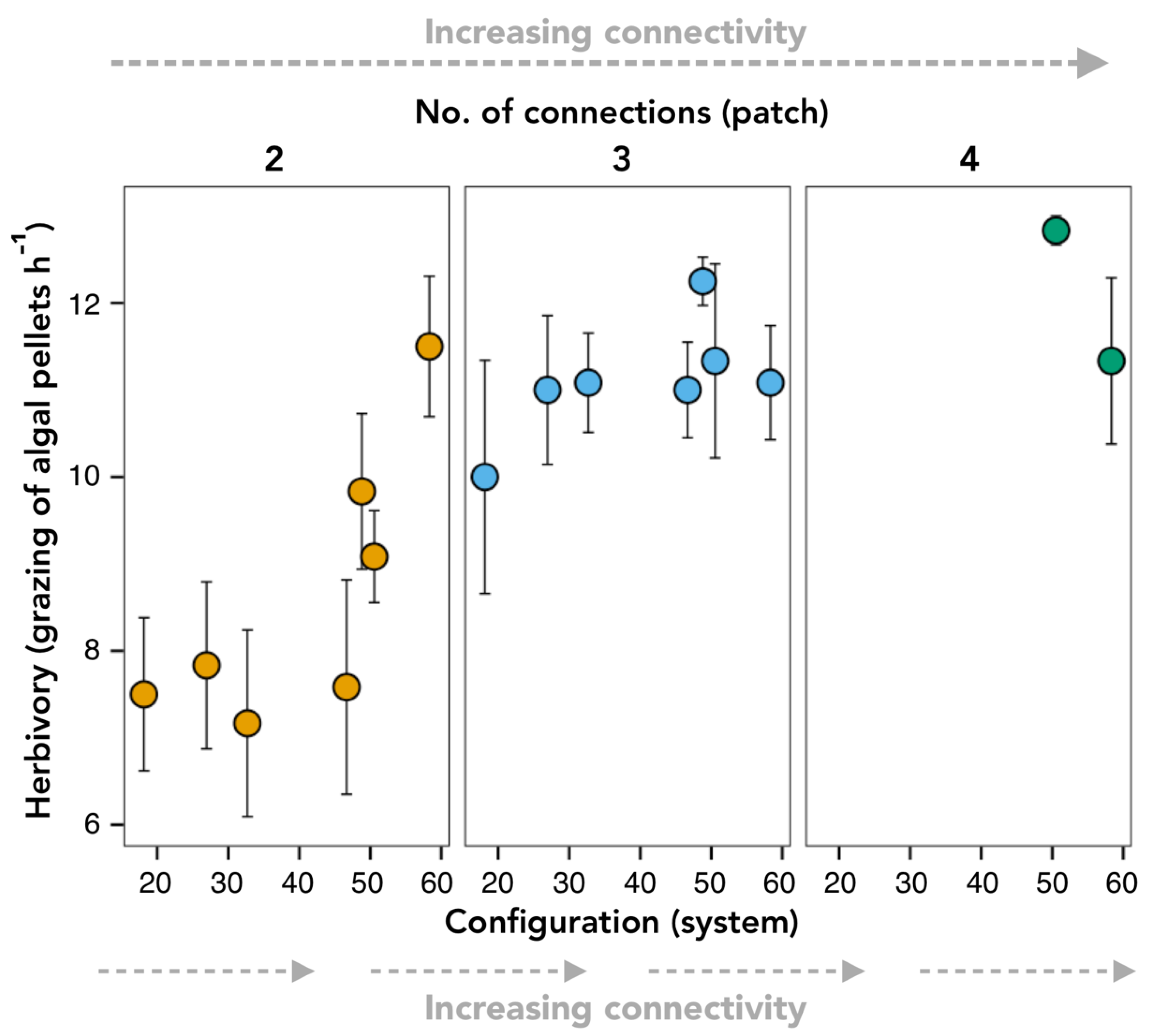
3.3. Variability in Grazing Rates

Grazing rates, at both the patch and system scale, were variable, possibly as a result of behavioural interactions (Figure 2 and Figure 3). We accounted for differences in the behaviour of crabs by including the replicate as a random effect in the analysis. It is, however, possible that some interactions between crabs were not explicitly addressed in the analysis. For example, competition may have impeded consumption rates by competitively inferior individuals in some patches; this is likely to occur in the field, and hence, our experiments mimic this scenario. Crowding near food patches may have constrained new arrivals to quickly access algal pellets, possibly lowering overall consumption rates for patches with many individuals. By contrast, increasing the number of connections provided alternative pathways to reach food patches, thereby making it more probable that more crabs would be the ‘first-on-scene’ at food patches.

4. Discussion

We show that herbivory increases with higher connectivity under both press and pulse disturbances in a controlled environment using a single model species. We tested two complementary metrics of connectivity (the number of connections and configuration); both were important predictors of herbivory at two spatial scales, the system and the patch. Herbivory by the hermit crab, Clibanarius virescens, was greater in better-connected systems and our results show that herbivory is best-predicted using both patch- and system-scale metrics of connectivity simultaneously, providing support for our first three hypotheses. We also found that configuration had a greater influence on herbivory during the press disturbance, supporting our fourth hypothesis. During the pulse disturbance, once a patch had three or four connections, the configuration of the system connections had little influence on herbivory in C. virescens (Figure 2). On the other hand, during the press disturbance, regardless of the number of system connections, the configuration of the patches continued to influence herbivory rates in C. virescens (Figure 3).
The finding that both the number and configuration of connections were important predictors for herbivory in disturbed experimental microcosms is supported by previous work. For example, the analysis of wildlife crossings planned for mitigation of the Trans-Canada highway upgrade resulted in two recommendations to increase potential movement of key species: (1) Increase the number (i.e., number of connections); and (2) change the location (i.e., configuration of connections) of crossings [44]. Analysing the effects of spatial configuration at the level of individual habitats, and at the landscape scale, has proven to be important in both terrestrial [44,45] and marine ecosystems [46,47,48]. The spatial configuration of habitat patches within marine networks is a key consideration for managers interested in improving the success of larval dispersal across marine networks [40]. The performance of restored habitats is also predicted to depend on the placement of restoration initiatives at sites with configurations that enhance the exchange of energy or individuals with other habitat patches [47,49]. Landscape configuration can also be used to predict movement patterns of important waterbird species, which help to maintain ecosystem functioning in fragmented landscapes [50]. The configuration of connections is an important consideration because it can influence how resources are accessed, used or even isolated within landscapes, thereby potentially contributing to the resilience of individual ecosystems and habitat patches [51].
The interaction between metrics for connectivity best-predicted the herbivory in response to both press and pulse disturbances. Determining which metric is the best predictor for a function, and considering connectivity at both the system and patch scale, might therefore be an important consideration for the management of any ecosystem [52,53]. For example, during the pulse disturbance, when a patch had a low number of connections (two) and low system configuration (20), grazing was low (<8 pellets h−1). However, in a patch with the same low number of connections (two), but high system configuration (60), more grazing occurred (>11 pellets h−1) (Figure 2). Knowledge of the spatial configuration of an entire system can, therefore, provide more accurate information about how much grazing might occur in a patch of interest, compared with simply measuring connections to neighbouring patches. This is supported by previous findings, which show that metrics indexing both system and patch measures of connectivity led to different conclusions about the viability of a population subject to habitat fragmentation, when compared with results from patch measures alone [54]. During the press disturbance, although the system with three connections had a high rate for grazing overall, patches with a lower value for configuration in that system had lower grazing rates than patches in a system with only one connection (Figure 3). These findings provide further evidence for management to consider whether they are interested in the functional response of a patch of interest, or the functional response of an overall system. Finally, when connectivity was high at both the patch and system scale, regardless of whether it was a press or pulse disturbance, herbivory remained high.
The variability in grazing rates, during both the press and pulse disturbance experiments, primarily reflects the complex nature of the relationship between connectivity and herbivory. It may, however, be further influenced by behavioural responses. Competition for a common resource by different species of herbivores in natural ecosystems is an important process that can control the growth and cover of algae in lake [55] and marine ecosystems [56]. The species of herbivore can also impact the type of algal consumption needed to maintain healthy reefs [57]. We acknowledge that the relationship between herbivory and the behaviour of herbivores is a complex process and can differ depending on the herbivore of interest, e.g., insect versus mammalian herbivory [58]. Therefore, it would be important to take into account the species of herbivores present in a natural ecosystem and their known behaviours when using this study as a baseline to test different levels and configurations of connectivity on the ecosystem function of herbivory.
Our results demonstrate that herbivory responds positively to increased connectivity and we have used herbivory to represent a positive effect that counteracts disturbance (i.e., excess algal growth) (Figure 4a). However, responses depend on whether the function responds positively or negatively to a disturbance in the system and the number of disturbances present in the system (summarised in Figure 4). In other situations, grazing can be detrimental to ecosystem integrity, such as excessive activity of sea urchins on coral reefs that can lower coral recruitment [59,60], which would result in a negative relationship with increasing connectivity (Figure 4b). Testing two (or more) opposing stressors together has the potential to determine whether intermediate levels of connectivity maximise resilience. For example, a combination of the positive effect of herbivore grazing for reef resilience [61] with the negative impacts from the spread of an invasive species [62] might result in a unimodal response (e.g., Figure 4c). A unimodal relationship has also been modelled in food web studies to highlight the opposing effects of prey protection with low connectivity and prey exploitation at higher levels of connectivity [63]. Further investigation is required to determine the impact that two opposing stressors might have in response to increasing connectivity.
A widely propagated design principle for experiments in ecology emphasises the pivotal role of robust inferences based on experimental conditions. Typically, ecologists seek to identify general relationships and distinguish such ‘generalities’ from inferences based on an idiosyncratic and narrow range of conditions [64]. It must be acknowledged that whilst no single experimental design will always be sufficient to define the broader generalities that ecologists seek [65], designs that achieve transferability of results to a broad range of settings and conditions will offer more robust and widely applicable insights. We used a single ecological function, herbivory, to test the effects of connectivity on ecological processes. Increasing connectivity in our experiment increased the rate of herbivory, and it is not implausible that other functions (e.g., predation, scavenging) may respond to connectivity in a similar manner under similar experimental conditions. For example, the availability of open corridors (higher connectivity) had a positive outcome for predators in a metacommunity experiment [12], further highlighting that extending our experimental design to other consumers and resources represents fertile ecological ground for future work.
Our conclusions are drawn from an experimental test performed in a controlled environment on one species, so further investigation is warranted to expand the findings beyond the limitations of a microcosm approach. The use of agal pellets as a proxy for herbivory in our model systems is a simplified way of measuring grazing. However, we feel its use is justified for several reasons. The algal pellets we used have a composition that reflects the natural algal diet of our model species and are of standardised weight and size, making it possible to accurately quantify and compare small changes in consumption rates between repeat measurements in a way that is difficult to achieve with live algae. Given our species responded well to this food source during acclimatisation, we believe it serves as a practical way of measuring consumption for the purposes used in this study. Future studies could consider building upon these findings by adding more complexity to food sources and model systems or by adding stressors. Despite the limitations and simple nature of our study, the techniques we have applied here could be replicated to test the way that other ecosystem functions and different species will respond to an increasing number and configuration of connectivity under other, single and multiple stressors/disturbances, and at different magnitudes. Different ecosystem processes, such as dispersal, habitat preference, competition, scavenging and predation, could affect these conclusions because ecosystems exhibit a wide range of characteristics [66]. Multiple stressors occurring simultaneously in a system may also result in antagonistic, synergistic or additive effects [67]. It would therefore be useful to test the connectivity relationship using multiple stressors that are likely to work antagonistically, synergistically and/or additively to determine how the functional response changes.

5. Conclusions

Our study suggests that connectivity at the system and patch scale are both important considerations for understanding grazer-mediated responses to press and pulse disturbances. We successfully designed and tested microcosm systems that allow testing of the ways that simple ecological systems respond to changes in linkages between spatially distinct units (mimicking habitat patches, islands or other parts of mosaics). Our experimental design opens opportunities to test multiple concepts of network theory for ecological systems in a way that is rarely possible to perform in the field (for logistical and ethical reasons). Furthermore, our experiments have practical applications for real-world scenarios. For example, in situations where effort has been made to restore important habitats that have failed (with little understanding as to why), our experiments show that there is potential value in analysing connectivity and configuration together. This type of analysis may help to uncover reasons for conservation failure where connectivity to other habitats is important for resistance or recovery from a disturbance. In a world where effective and efficient conservation designs will become increasingly critical in the face of mounting human threats, enhancing such designs by applying more robust connectivity criteria will be a useful input that can benefit from conceptual advances made in controlled experiments.

Supplementary Materials

The following are available online at https://www.mdpi.com/1424-2818/12/11/424/s1, Figure S1: Example of experimental microcosm.

Author Contributions

Conceptualization, T.A.S., A.D.O. and R.M.C.; data curation, K.I.J.; formal analysis, K.I.J., C.J.B. and R.M.P.; funding acquisition, T.A.S. and R.M.C.; investigation, K.I.J.; methodology, K.I.J., S.L.E. and R.M.C.; project administration, K.I.J.; resources, T.A.S. and R.M.C.; supervision, C.J.B., S.L.E. and R.M.C.; validation, K.I.J.; visualization, K.I.J.; writing—original draft, K.I.J.; writing—review and editing, K.I.J., C.J.B., T.A.S., A.D.O., S.L.E., R.M.P. and R.M.C. All authors have read and agreed to the published version of the manuscript.

Funding

R.M.C. and T.A.S. were funded by an Australian Research Council Discovery Project, grant number DP150102271; C.J.B. was funded by an Australian Research Council Discovery Early Career Researcher Award, grant number DE160101207; K.I.J. was funded by an Australian Rivers Institute Scholarship.

Conflicts of Interest

The authors declare no conflict of interest. The funders had no role in the design of the study; in the collection, analyses, or interpretation of data; in the writing of the manuscript, or in the decision to publish the results.

Appendix A

Appendix A.1. Network Theory Metrics Used to Measure Configuration at the Patch and System Scale

Closeness centrality [1] is a network theory metric that we adapted to calculate a value for the configuration of the patches and systems for analysis of our experimental microcosms. Closeness centrality is the inverse of the sum of the shortest path between the patch of interest and all other patches in the system, measured as the number of links (or topographical distance) in the microcosms used here.

Appendix A.2. Patch-Scale Configuration Metric

At the patch scale, we adapted closeness centrality to the following measure for configuration:
Configuration   ( patch ) =   [ i = 1 n d ( p k ,   p i ) ] 1 × 100
where:
  • p k = disturbed patch of interest (A, B, C or D (Figure A1))
  • p i = all undisturbed patches (U1, U2, U3, U4 and U5 (Figure A1))
  • d ( p i ,   p k ) = the number of links (topographical distance) between p k and p i
We modified the original equation for closeness centrality developed by Freeman [36] in two ways:
  • In the original equation, pi refers to all other patches within the system; however, because we were only interested in the grazing power of the crabs coming from the undisturbed patches to each of the disturbed patches, our measure for patch configuration considers only the connectivity between the disturbed patch of interest and all undisturbed patches (Figure A1);
  • Due to the limited number of patches and overall size of our system, closeness values were in the order of 1 × 10⁻³; therefore, we multiplied the original equation by 100 to obtain an easily interpretable value.
Figure A1. (a): Experimental systems showing the disturbed patches, A–D in white, and undisturbed patches, U1–U5 in grey; (b): Example showing the patches (indicated by arrows) used to calculate configuration at the patch scale for a disturbed patch, A (circled).
Diversity 12 00424 g0a1

Appendix A.3. System-Scale Configuration Metric

At the whole-of-system scale, we varied the number and spatial arrangement of the connections linking disturbed and undisturbed patches. We combined two measures to represent ‘configuration’ at the system scale, to account for the way these connections increased in connectivity, and to account for the direction of the migration of animals through the system: (1) the average configuration of each undisturbed patch to each of the disturbed patches; and (2) the probability that a crab would walk in the right direction toward a disturbed patch to graze.
For the first measure, the average configuration, we were interested in how closely connected all of the undisturbed patches were to the disturbed patches; thus, we adapted closeness centrality as follows:
x ¯   closeness   ( U 1 : U 5 )   =   [ i = 1 n d ( p u ,   p d ) ] 1 × 100
where:
  • p u = undisturbed patch of interest (U1, U2, U3, U4 or U5 (Figure A2))
  • p d = all disturbed patches (white patches in Figure A2)
  • d ( p u ,   p d ) = the number of links (topographical distance) between p u and p d
Figure A2. (a): Example showing the patches (indicated by arrows) used to calculate configuration for U1 (circled) (e.g., distance between U1 and all disturbed patches (in white)), with the average distance from U1 to U5 used to provide a configuration value; (b): Example system showing the probability in each undisturbed patch that the crab will move in the right direction toward a disturbed patch.
Diversity 12 00424 g0a2
For the second measure, we then summed the probability that each of the five crabs in undisturbed patches (U1:U5) would take the correct path toward a disturbed patch to graze (Figure A2). For example, if a patch has two connections and only one of those connections takes the crab in the right direction (towards a disturbed patch with excess algae) to graze, then that patch has a probability of ½; therefore, our equation is as follows:
P U 1 : U 5   =   N o .   o f   c o r r e c t   p a t h s T o t a l   n u m b e r   o f   p a t h s
Finally, these two measures were multiplied to provide our overall metric for configuration at the system scale:
Configuration   ( system ) = x ¯   closeness   ( U 1 : U 5 ) × P U 1 : U 5
Connectivity metrics for each of the systems at the patch and system scale are shown in Table 1.

References

  1. Beger, M.; Grantham, H.S.; Pressey, R.L.; Wilson, K.A.; Peterson, E.L.; Dorfman, D.; Mumby, P.J.; Lourival, R.; Brumbaugh, D.R.; Possingham, H.P. Conservation planning for connectivity across marine, freshwater, and terrestrial realms. Biol. Conserv. 2010, 143, 565–575. [Google Scholar] [CrossRef]
  2. Filbee-Dexter, K.; Wernberg, T.; Norderhaug, K.M.; Ramirez-Llodra, E.; Pedersen, M.F. Movement of pulsed resource subsidies from kelp forests to deep fjords. Oecologia 2018, 187, 291–304. [Google Scholar] [CrossRef] [Green Version]
  3. Adam, T.C.; Schmitt, R.J.; Holbrook, S.J.; Brooks, A.J.; Edmunds, P.J.; Carpenter, R.C.; Bernardi, G. Herbivory, connectivity, and ecosystem resilience: Response of a coral reef to a large-scale perturbation. PLoS ONE 2011, 6, e23717. [Google Scholar] [CrossRef] [PubMed]
  4. Magioli, M.; de Barros, K.M.P.M.; Setz, E.Z.F.; Percequillo, A.R.; Rondon, M.V.D.S.S.; Kuhnen, V.V.; Da Silva Canhoto, M.C.; Dos Santos, K.E.A.; Kanda, C.Z.; de Lima Fregonezi, G.; et al. Connectivity maintain mammal assemblages functional diversity within agricultural and fragmented landscapes. Eur. J. Wildl. Res. 2016, 62, 431–446. [Google Scholar] [CrossRef] [Green Version]
  5. Westwood, A.R.; Lambert, J.D.; Reitsma, L.R.; Stralberg, D. Prioritizing areas for land conservation and forest management planning for the threatened Canada Warbler (Cardellina canadensis) in the Atlantic Northern Forest of Canada. Diversity 2020, 12, 61. [Google Scholar] [CrossRef] [Green Version]
  6. Mitchell, M.G.E.; Bennett, E.M.; Gonzalez, A. Linking landscape connectivity and ecosystem service provision: Current knowledge and research gaps. Ecosystems 2013, 16, 894–908. [Google Scholar] [CrossRef]
  7. Noël, L.M.L.J.; Hawkins, S.J.; Jenkins, S.R.; Thompson, R.C. Grazing dynamics in intertidal rockpools: Connectivity of microhabitats. J. Exp. Mar. Bio. Ecol. 2009, 370, 9–17. [Google Scholar] [CrossRef]
  8. Olds, A.D.; Pitt, K.A.; Maxwell, P.S.; Connolly, R.M.; Frid, C. Synergistic effects of reserves and connectivity on ecological resilience. J. Appl. Ecol. 2012, 49, 1195–1203. [Google Scholar] [CrossRef]
  9. Ruiz-Montoya, L.; Lowe, R.J.; Kendrick, G.A. Contemporary connectivity is sustained by wind- and current-driven seed dispersal among seagrass meadows. Mov. Ecol. 2015, 3, 9. [Google Scholar] [CrossRef]
  10. Schlacher, T.A.; Strydom, S.; Connolly, R.M.; Schoeman, D. Donor-control of scavenging food webs at the land-ocean interface. PLoS ONE 2013, 8, e68221. [Google Scholar] [CrossRef] [Green Version]
  11. Treml, E.A.; Ford, J.R.; Black, K.P.; Swearer, S.E. Identifying the key biophysical drivers, connectivity outcomes, and metapopulation consequences of larval dispersal in the sea. Mov. Ecol. 2015, 3, 17. [Google Scholar] [CrossRef] [PubMed] [Green Version]
  12. Limberger, R.; Wickham, S.A. Predator dispersal determines the effect of connectivity on prey diversity. PLoS ONE 2011, 6, e29071. [Google Scholar] [CrossRef] [PubMed]
  13. Acevedo, M.A.; Fletcher, R.J., Jr.; Tremblay, R.L.; Melendez-Ackerman, E.J. Spatial asymmetries in connectivity influence colonization-extinction dynamics. Oecologia 2015, 179, 415–424. [Google Scholar] [CrossRef]
  14. Elmhirst, T.; Connolly, S.R.; Hughes, T.P. Connectivity, regime shifts and the resilience of coral reefs. Coral Reefs 2009, 28, 949–957. [Google Scholar] [CrossRef]
  15. Hogan, J.D.; Thiessen, R.J.; Sale, P.F.; Heath, D.D. Local retention, dispersal and fluctuating connectivity among populations of a coral reef fish. Oecologia 2012, 168, 61–71. [Google Scholar] [CrossRef] [Green Version]
  16. Elmqvist, T.; Folke, C.; Nystrom, M.; Peterson, G.; Bengtsson, J.; Walker, B.; Norberg, J. Response diversity, ecosystem change, and resilience. Front. Ecol. Environ. 2003, 1, 488–494. [Google Scholar] [CrossRef]
  17. Mumby, P.J.; Elliott, I.A.; Eakin, C.M.; Skirving, W.; Paris, C.B.; Edwards, H.J.; Enriquez, S.; Iglesias-Prieto, R.; Cherubin, L.M.; Stevens, J.R. Reserve design for uncertain responses of coral reefs to climate change. Ecol. Lett. 2011, 14, 132–140. [Google Scholar] [CrossRef]
  18. Dikou, A. Ecological processes and contemporary coral reef management. Diversity 2010, 2, 717–737. [Google Scholar] [CrossRef]
  19. Vergés, A.; McCosker, E.; Mayer-Pinto, M.; Coleman, M.A.; Wernberg, T.; Ainsworth, T.; Steinberg, P.D.; Williams, G. Tropicalisation of temperate reefs: Implications for ecosystem functions and management actions. Funct. Ecol. 2019. [Google Scholar] [CrossRef] [Green Version]
  20. Fox, R.J.; Bellwood, D.R. Quantifying herbivory across a coral reef depth gradient. Mar. Ecol. Prog. Ser. 2007, 339, 49–59. [Google Scholar] [CrossRef]
  21. Cheal, A.J.; MacNeil, M.A.; Cripps, E.; Emslie, M.J.; Jonker, M.; Schaffelke, B.; Sweatman, H. Coral–macroalgal phase shifts or reef resilience: Links with diversity and functional roles of herbivorous fishes on the Great Barrier Reef. Coral Reefs 2010, 29, 1005–1015. [Google Scholar] [CrossRef]
  22. Poore, A.G.; Campbell, A.H.; Coleman, R.A.; Edgar, G.J.; Jormalainen, V.; Reynolds, P.L.; Sotka, E.E.; Stachowicz, J.J.; Taylor, R.B.; Vanderklift, M.A.; et al. Global patterns in the impact of marine herbivores on benthic primary producers. Ecol. Lett. 2012, 15, 912–922. [Google Scholar] [CrossRef]
  23. Ebrahim, A.; Olds, A.D.; Maxwell, P.S.; Pitt, K.A.; Burfeind, D.D.; Connolly, R.M. Herbivory in a subtropical seagrass ecosystem: Separating the functional role of different grazers. Mar. Ecol. Prog. Ser. 2014, 511, 83–91. [Google Scholar] [CrossRef] [Green Version]
  24. Hoffmann, L.; Edwards, W.; York, P.H.; Rasheed, M.A. Richness of primary producers and consumer abundance mediate epiphyte loads in a tropical seagrass system. Diversity 2020, 12, 384. [Google Scholar] [CrossRef]
  25. Martin, T.S.H.; Olds, A.D.; Olalde, A.B.H.; Berkström, C.; Gilby, B.L.; Schlacher, T.A.; Butler, I.R.; Yabsley, N.A.; Zann, M.; Connolly, R.M. Habitat proximity exerts opposing effects on key ecological functions. Landsc. Ecol. 2018, 33, 1273–1286. [Google Scholar] [CrossRef] [Green Version]
  26. Engelhard, S.L.; Huijbers, C.M.; Stewart-Koster, B.; Olds, A.D.; Schlacher, T.A.; Connolly, R.M.; Österblom, H. Prioritising seascape connectivity in conservation using network analysis. J. Appl. Ecol. 2017, 54, 1130–1141. [Google Scholar] [CrossRef] [Green Version]
  27. Kindlmann, P.; Burel, F. Connectivity measures: A review. Landsc. Ecol. 2008, 23, 879–890. [Google Scholar] [CrossRef] [Green Version]
  28. Driver, L.J.; Hoeinghaus, D.J. Fish metacommunity responses to experimental drought are determined by habitat heterogeneity and connectivity. Freshw. Biol. 2016, 61, 533–548. [Google Scholar] [CrossRef]
  29. Gilarranz, L.J.; Rayfield, B.; Linan-Cembrano, G.; Bascompte, J.; Gonzalez, A. Effects of network modularity on the spread of perturbation impact in experimental metapopulations. Science 2017, 357, 199–201. [Google Scholar] [CrossRef] [Green Version]
  30. Limberger, R.; Wickham, S.A. Transitory versus persistent effects of connectivity in environmentally homogeneous metacommunities. PLoS ONE 2012, 7, e44555. [Google Scholar] [CrossRef] [Green Version]
  31. Di Carvalho, J.A.; Wickham, S.A. Simulating eutrophication in a metacommunity landscape: An aquatic model ecosystem. Oecologia 2019, 189, 461–474. [Google Scholar] [CrossRef] [PubMed] [Green Version]
  32. Pearson, R.M.; Jinks, K.I.; Brown, C.J.; Schlacher, T.A.; Connolly, R.M. Functional changes in reef systems in warmer seas: Asymmetrical effects of altered grazing by a widespread crustacean mesograzer. Sci. Total Environ. 2018, 644, 976–981. [Google Scholar] [CrossRef]
  33. Schlacher, T.A.; Skillington, A.J.; Connolly, R.M.; Robinson, W.; Gaston, T.F. Coupling between marine plankton and freshwater flow in the plumes off a small estuary. Int. Rev. Hydrobiol. 2008, 93, 641–658. [Google Scholar] [CrossRef]
  34. Wainger, L.; Yu, H.; Gazenski, K.; Boynton, W. The relative influence of local and regional environmental drivers of algal biomass (chlorophyll-a) varies by estuarine location. Estuar. Coast. Shelf Sci. 2016, 178, 65–76. [Google Scholar] [CrossRef]
  35. Yabsley, N.A.; Olds, A.D.; Connolly, R.M.; Martin, T.S.; Gilby, B.L.; Maxwell, P.S.; Huijbers, C.M.; Schoeman, D.S.; Schlacher, T.A. Resource type influences the effects of reserves and connectivity on ecological functions. J. Anim. Ecol. 2016, 85, 437–444. [Google Scholar] [CrossRef] [PubMed] [Green Version]
  36. Freeman, L.C. Centrality in social networks conceptual clarification. Soc. Netw. 1979, 1, 215–239. [Google Scholar] [CrossRef] [Green Version]
  37. Latora, V.; Marchiori, M. Efficient behavior of small-world networks. Phys. Rev. Lett. 2001, 87, 198701. [Google Scholar] [CrossRef] [Green Version]
  38. Saunders, M.I.; Brown, C.J.; Foley, M.M.; Febria, C.M.; Albright, R.; Mehling, M.G.; Kavanaugh, M.T.; Burfeind, D.D. Human impacts on connectivity in marine and freshwater ecosystems assessed using graph theory: A review. Mar. Freshw. Res. 2016, 67, 277–290. [Google Scholar] [CrossRef] [Green Version]
  39. Tavella, J.; Cagnolo, L. Does fire disturbance affect ant community structure? Insights from spatial co-occurrence networks. Oecologia 2019. [Google Scholar] [CrossRef]
  40. Treml, E.A.; Halpin, P.N.; Urban, D.L.; Pratson, L.F. Modeling population connectivity by ocean currents, a graph-theoretic approach for marine conservation. Landsc. Ecol. 2007, 23, 19–36. [Google Scholar] [CrossRef]
  41. Beger, M.; Linke, S.; Watts, M.; Game, E.; Treml, E.; Ball, I.; Possingham, H.P. Incorporating asymmetric connectivity into spatial decision making for conservation. Conserv. Lett. 2010, 3, 359–368. [Google Scholar] [CrossRef]
  42. Bates, D.; Maechler, M.; Bolker, B.; Walker, S.; Christensen, R.H.B.; Singmann, H.; Dai, B.; Grothendieck, G.; Green, P. lme4: Linear Mixed-Effects Models Using ‘Eigen’ and S4; R package ver. 1.1-12; R Foundation for Statistical Computing: Vienna, Austria, 2016. [Google Scholar]
  43. R Core Team. R: A Language and Environment for Statistical Computing; R Foundation for Statistical Computing: Vienna, Austria, 2017. [Google Scholar]
  44. Alexander, S.M. Snow-tracking and GIS: Using multiple species-environment models to determine optimal wildlife crossing sites and evaluate highway mitigation plans on the Trans-Canada Highway. Can. Geogr. 2008, 52, 169–187. [Google Scholar] [CrossRef]
  45. Nabe-Nielsen, J.; Sibly, R.M.; Forchhammer, M.C.; Forbes, V.E.; Topping, C.J. The effects of landscape modifications on the long-term persistence of animal populations. PLoS ONE 2010, 5, e8932. [Google Scholar] [CrossRef] [PubMed] [Green Version]
  46. Dorenbosch, M.; Verberk, W.; Nagelkerken, I.; van der Velde, G. Influence of habitat configuration on connectivity between fish assemblages of Caribbean seagrass beds, mangroves and coral reefs. Mar. Ecol. Prog. Ser. 2007, 334, 103–116. [Google Scholar] [CrossRef] [Green Version]
  47. Gilby, B.L.; Olds, A.D.; Connolly, R.M.; Henderson, C.J.; Schlacher, T.A. Spatial restoration ecology: Placing restoration in a landscape context. BioScience 2018, 68, 1007–1019. [Google Scholar] [CrossRef]
  48. Olds, A.D.; Connolly, R.M.; Pitt, K.A.; Maxwell, P.S. Primacy of seascape connectivity effects in structuring coral reef fish assemblages. Mar. Ecol. Prog. Ser. 2012, 462, 191–203. [Google Scholar] [CrossRef] [Green Version]
  49. Duncan, C.K.; Gilby, B.L.; Olds, A.D.; Connolly, R.M.; Ortodossi, N.L.; Henderson, C.J.; Schlacher, T.A. Landscape context modifies the rate and distribution of predation around habitat restoration sites. Biol. Conserv. 2019, 237, 97–104. [Google Scholar] [CrossRef]
  50. Kleyheeg, E.; van Dijk, J.G.B.; Tsopoglou-Gkina, D.; Woud, T.Y.; Boonstra, D.K.; Nolet, B.A.; Soons, M.B. Movement patterns of a keystone waterbird species are highly predictable from landscape configuration. Mov. Ecol. 2017, 5, 2. [Google Scholar] [CrossRef] [Green Version]
  51. Bodin, Ö.; Tengö, M. Disentangling intangible social–ecological systems. Glob. Environ. Chang. 2012, 22, 430–439. [Google Scholar] [CrossRef]
  52. Crook, D.A.; Lowe, W.H.; Allendorf, F.W.; Erős, T.; Finn, D.S.; Gillanders, B.M.; Hadwen, W.L.; Harrod, C.; Hermoso, V.; Jennings, S.; et al. Human effects on ecological connectivity in aquatic ecosystems: Integrating scientific approaches to support management and mitigation. Sci. Total Environ. 2015, 534, 52–64. [Google Scholar] [CrossRef] [Green Version]
  53. Rudnick, D.A.; Ryan, S.J.; Beier, P.; Cushman, S.A.; Dieffenbach, F.; Epps, C.W.; Gerber, L.R.; Hartter, J.; Jenness, J.S.; Kintsch, J.; et al. The role of landscape connectivity in planning and implementing conservation and restoration priorities. Issues Ecol. 2012, 16, 1–20. [Google Scholar]
  54. Ferrari, J.R.; Lookingbill, T.R.; Neel, M.C. Two measures of landscape-graph connectivity: Assessment across gradients in area and configuration. Landsc. Ecol. 2007, 22, 1315–1323. [Google Scholar] [CrossRef]
  55. Vejrikova, I.; Vejrik, L.; Leps, J.; Kocvara, L.; Sajdlova, Z.; Ctvrtlikova, M.; Peterka, J. Impact of herbivory and competition on lake ecosystem structure: Underwater experimental manipulation. Sci. Rep. 2018, 8, 12130. [Google Scholar] [CrossRef]
  56. Hay, M.E.; Taylor, P.R. Competition between herbivorous fishes and urchins on Caribbean reefs. Oecologia 1985, 65, 591–598. [Google Scholar] [CrossRef]
  57. Humphries, A.T.; McClanahan, T.R.; McQuaid, C.D. Algal turf consumption by sea urchins and fishes is mediated by fisheries management on coral reefs in Kenya. Coral Reefs 2020, 39, 1137–1146. [Google Scholar] [CrossRef]
  58. Hambäck, P.A.; Beckerman, A.P. Herbivory and plant resource competition: A review of two interacting interactions. Oikos 2003, 101, 26–37. [Google Scholar] [CrossRef]
  59. Korzen, L.; Israel, A.; Abelson, A. Grazing effects of fish versus sea urchins on turf algae and coral recruits: Possible omplications for coral reef resilience and restoration. J. Mar. Biol. 2011, 2011, 1–8. [Google Scholar] [CrossRef] [Green Version]
  60. Norström, A.V.; Nyström, M.; Lokrantz, J.; Folke, C. Alternative states on coral reefs: Beyond coral–macroalgal phase shifts. Mar. Ecol. Prog. Ser. 2009, 376, 295–306. [Google Scholar] [CrossRef]
  61. Mumby, P.J.; Hastings, A. The impact of ecosystem connectivity on coral reef resilience. J. Appl. Ecol. 2007, 45, 854–862. [Google Scholar] [CrossRef]
  62. Hock, K.; Wolff, N.H.; Condie, S.A.; Anthony, K.R.N.; Mumby, P.J.; Paynter, Q. Connectivity networks reveal the risks of crown-of-thorns starfish outbreaks on the Great Barrier Reef. J. Appl. Ecol. 2014, 51, 1188–1196. [Google Scholar] [CrossRef] [Green Version]
  63. LeCraw, R.M.; Kratina, P.; Srivastava, D.S. Food web complexity and stability across habitat connectivity gradients. Oecologia 2014, 176, 903–915. [Google Scholar] [CrossRef]
  64. Wenger, S.J.; Olden, J.D. Assessing transferability of ecological models: An underappreciated aspect of statistical validation. Methods Ecol. Evol. 2012, 3, 260–267. [Google Scholar] [CrossRef]
  65. Beck, M.W. Inference and generality in ecology: Current problems and an experimental solution. Oikos 1997, 78, 265–273. [Google Scholar] [CrossRef]
  66. Loreau, M.; de Mazancourt, C. Biodiversity and ecosystem stability: A synthesis of underlying mechanisms. Ecol. Lett. 2013, 16 (Suppl. 1), 106–115. [Google Scholar] [CrossRef] [PubMed]
  67. Côte, I.M.; Darling, E.S.; Brown, C.J. Interactions among ecosystem stressors and their importance in conservation. Proc. R. Soc. B 2016, 283, 20152592. [Google Scholar] [CrossRef] [PubMed]
Figure 1. Experimental microcosms with different levels of connectivity that did not mirror each other. Connectivity increases with respect to an increasing number of links between the undisturbed and disturbed part of the system, and with respect to alternative spatial configurations for a given number of links.
Diversity 12 00424 g001
Figure 2. Herbivory during a pulse disturbance and the interaction between patch- and system-scale responses to an increase in connectivity. Herbivory is the mean (SE) number of algal pellets consumed after a 1 h period (colours indicate no. of connections at the patch scale). No. of connections (patch) is the number of connections that linked disturbed patches to neighbouring patches (disturbed patches had a minimum of two connections). Configuration (system) is a modified value for closeness centrality at the system scale, which quantifies a commonly used dimension of connectivity.
Diversity 12 00424 g002
Figure 3. Herbivory during a press disturbance and the interaction between patch- and system-scale responses to an increase in connectivity. Herbivory is the mean (SE) number of algal pellets consumed after a 7 h period of a consistent supply of algae to disturbed patches in each system (colours indicate no. of connections at the system scale). No. of connections (system) is the number of connections linking the undisturbed to the disturbed part of the system. Configuration (patch) is a modified value for closeness centrality at the patch scale, which quantifies a commonly used dimension of connectivity.
Diversity 12 00424 g003
Figure 4. Conceptual models illustrating three examples of how an ecological function (e.g., herbivory as tested in this study) may respond to increasing levels of connectivity. The function can respond either positively (a) or negatively (b) to increased connectivity, either linearly (sold line) or exhibiting an upper (dashed line) or lower threshold (dotted line). A unimodal response curve (c) could occur where a function (or multiple functions) responds initially positively to more connectivity but declines beyond a certain threshold of connectivity. Positive relationships are indicated with blue lines and negative relationships with red lines.
Diversity 12 00424 g004
Table 1. Experimental system setups with patch- and system-scale connectivity values for the ‘number of connections’ and ‘configuration’ of the connections. Number of connections at the system scale is the number of links between disturbed patches (A–D) and undisturbed patches (grey), and number of connections at the patch scale is the number of neighbouring patches to the patch of interest (A–D). Values for configuration at the patch scale and system scale are calculated using an adaptation of the network theory measure of closeness centrality from Freeman [36]. Red arrows indicate open connections.
Model SystemSystem ScalePatchPatch Scale
No. of ConnectionsConfigurationNo. of ConnectionsConfiguration
1 Diversity 12 00424 i001118.1A
B
C
D
3
2
2
2
5.3
4.2
4.2
3.4
2 Diversity 12 00424 i002126.9A
B
C
D
2
2
3
2
4.8
3.8
6.3
4.8
3 Diversity 12 00424 i003232.7A
B
C
D
3
2
3
2
5.3
4.2
6.3
4.8
4 Diversity 12 00424 i004246.7A
B
C
D
3
2
3
2
6.7
5.0
7.1
5.3
5 Diversity 12 00424 i005248.8A
B
C
D
3
2
2
3
5.9
5.6
5.6
5.9
6 Diversity 12 00424 i006350.6A
B
C
D
3
2
4
2
6.7
5.0
8.3
5.9
7 Diversity 12 00424 i007458.3A
B
C
D
3
2
4
3
6.7
5.6
8.3
6.7
Table 2. Summary of experimental parameters for microcosms testing the effect of connectivity on herbivory. Microcosms were designed so that connectivity varied between disturbed and undisturbed patches in various ways.
ExperimentPulse Press
Length of experiment1 h7 h
No. of crabs per patch11
No. of patches per system99
No. of pellets added per hour to undisturbed patches (×5)11
No. of pellets added per hour to disturbed patches (×4)139
Table 3. The number of connections and configuration at the patch and system scale significantly increased herbivory (p < 0.05 for all models). Best models for herbivory in response to pulse and press disturbances are in bold, determined using the difference in Akaike Information Criterion (AIC) values from generalised linear mixed models; Δi. Akaike weights (AICW) are used to show the probability that the model is better than those being compared. No. of connections = number of connections between undisturbed and disturbed patches at the system level or number of direct connections to individual patches.
ExperimentLevelConnectivity Measure TestedAICAICW
Pulse disturbancePatchNo. of connections8400.06
Configuration8470.06
SystemNo. of connections9670.00
Configuration9640.00
AdditiveNo. of connections(patch) + Configuration(system) 8390.10
InteractionNo. of connections(patch) × Configuration(system)8350.77
Press disturbancePatchNo. of connections18390.00
Configuration18190.07
SystemNo. of connections20180.00
Configuration20200.00
AdditiveConfiguration(patch) + No. of connections(system)18210.03
InteractionConfiguration(patch) × No. of connections(system)18140.90
Publisher’s Note: MDPI stays neutral with regard to jurisdictional claims in published maps and institutional affiliations.

