
The Effects of Random Porosities in Resonant Frequencies of Graphene Based on the Monte Carlo Stochastic Finite Element Model


Abstract
:1. Introduction
2. Results and Discussion
2.1. Statistical Results
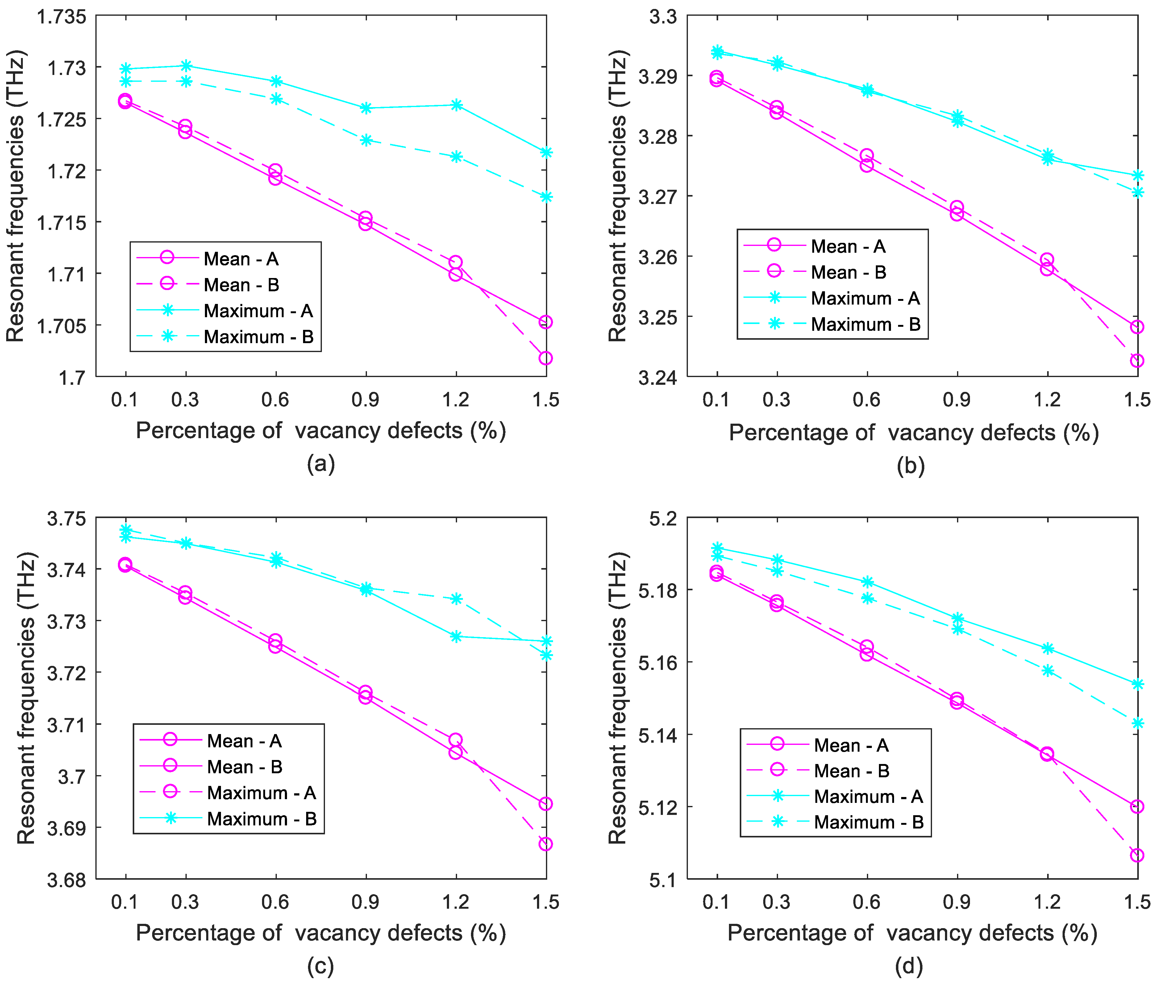
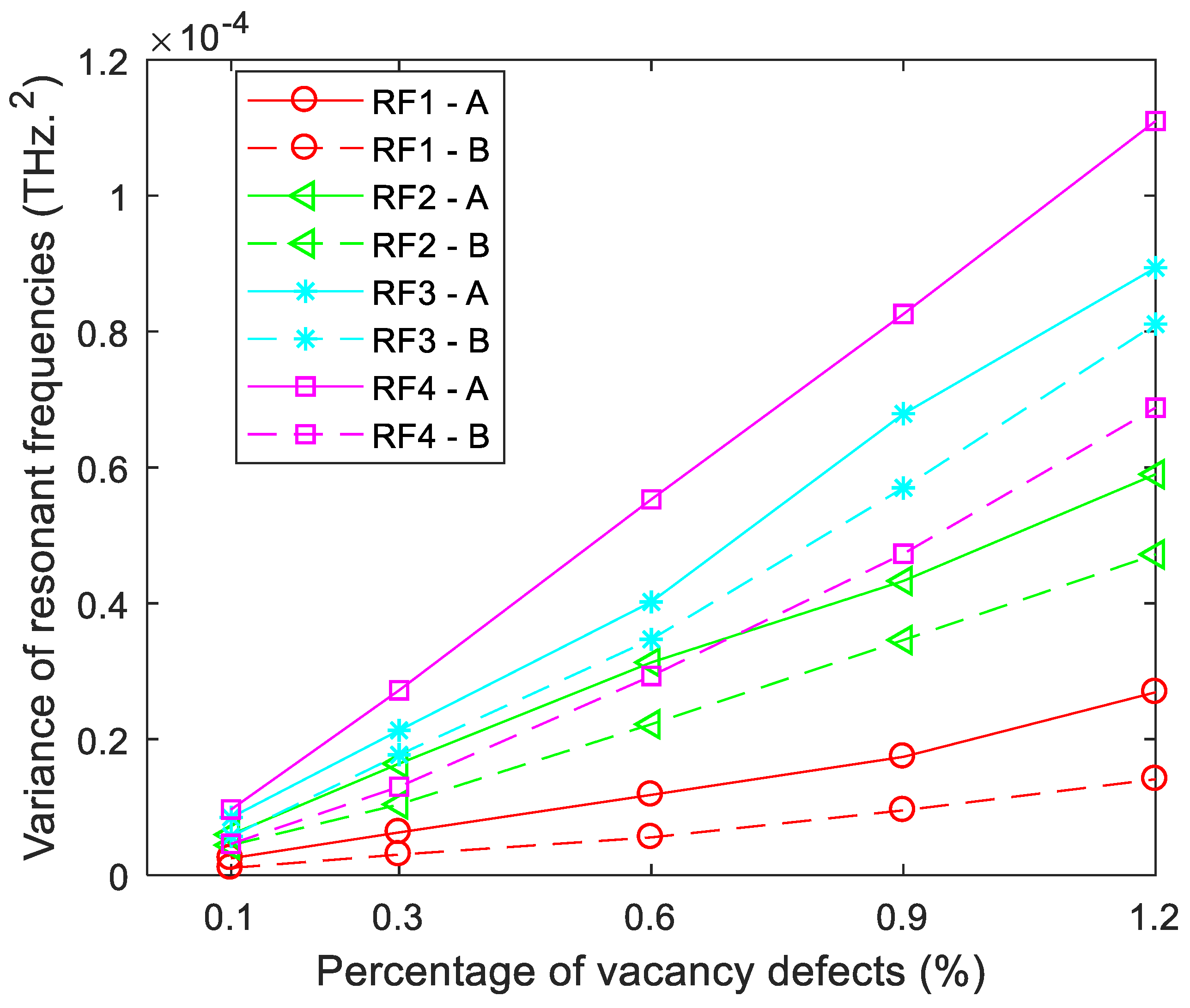
2.2. Comparison and Discussion
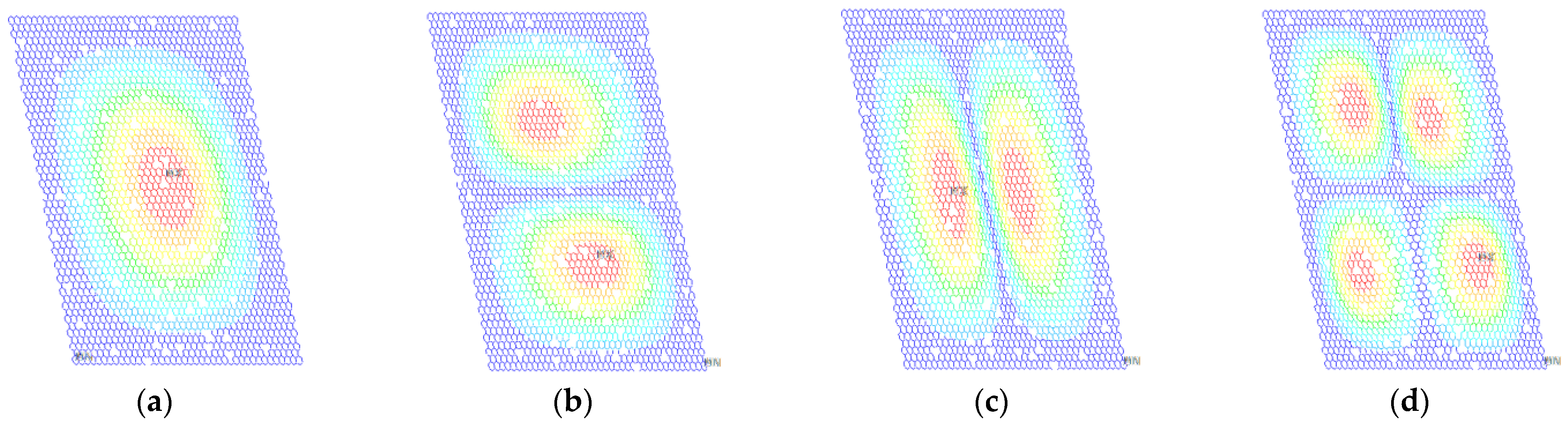
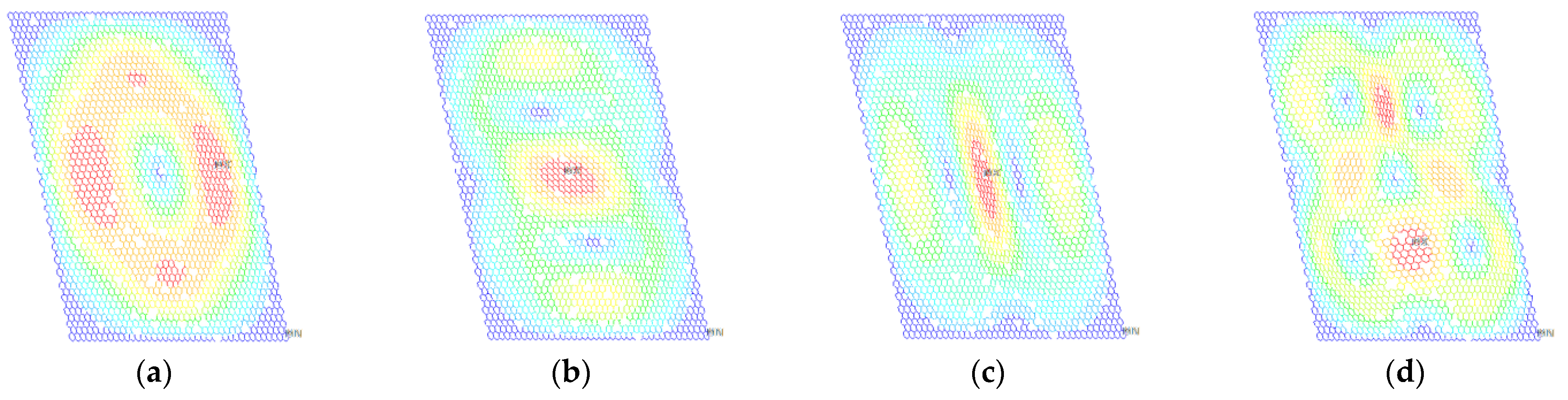
2.3. Vibration Modes of Porous Graphene
3. Materials and Methods
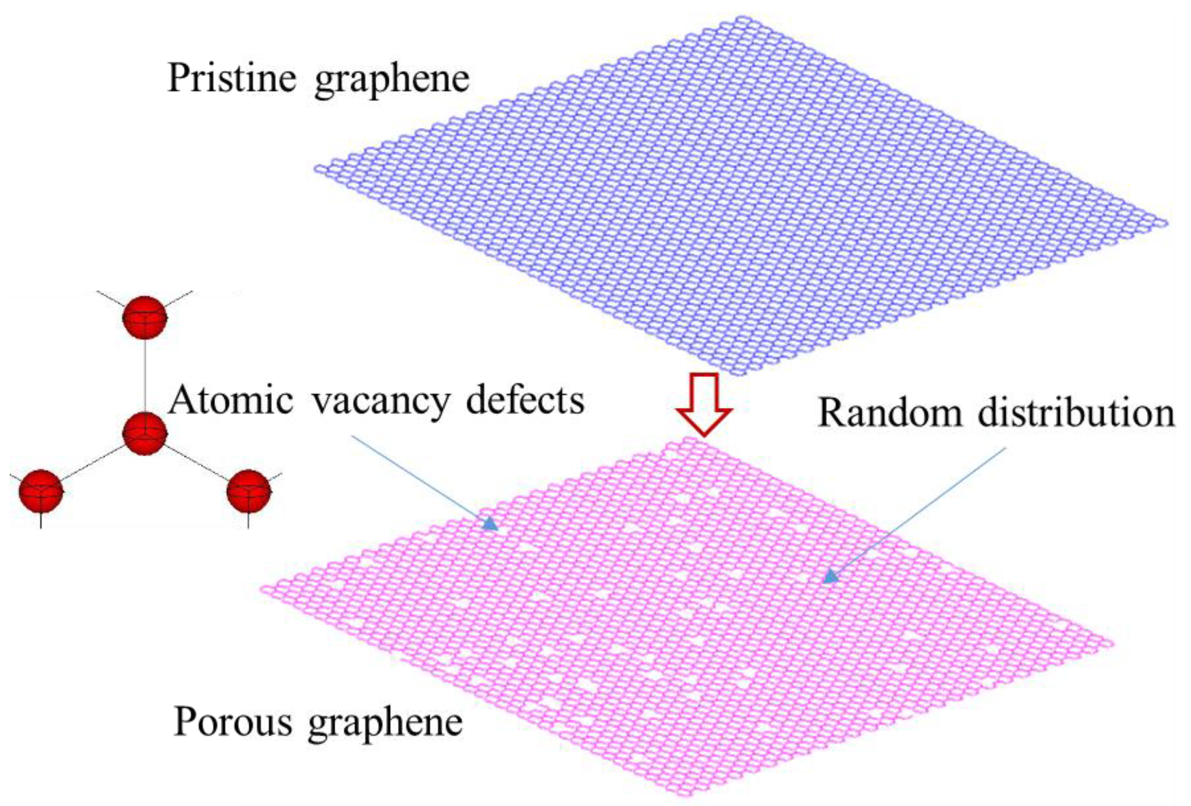
3.1. Porous Graphene
3.2. Beam Finite Element
3.3. Monte Carlo-Based Finite Element Method
4. Conclusions
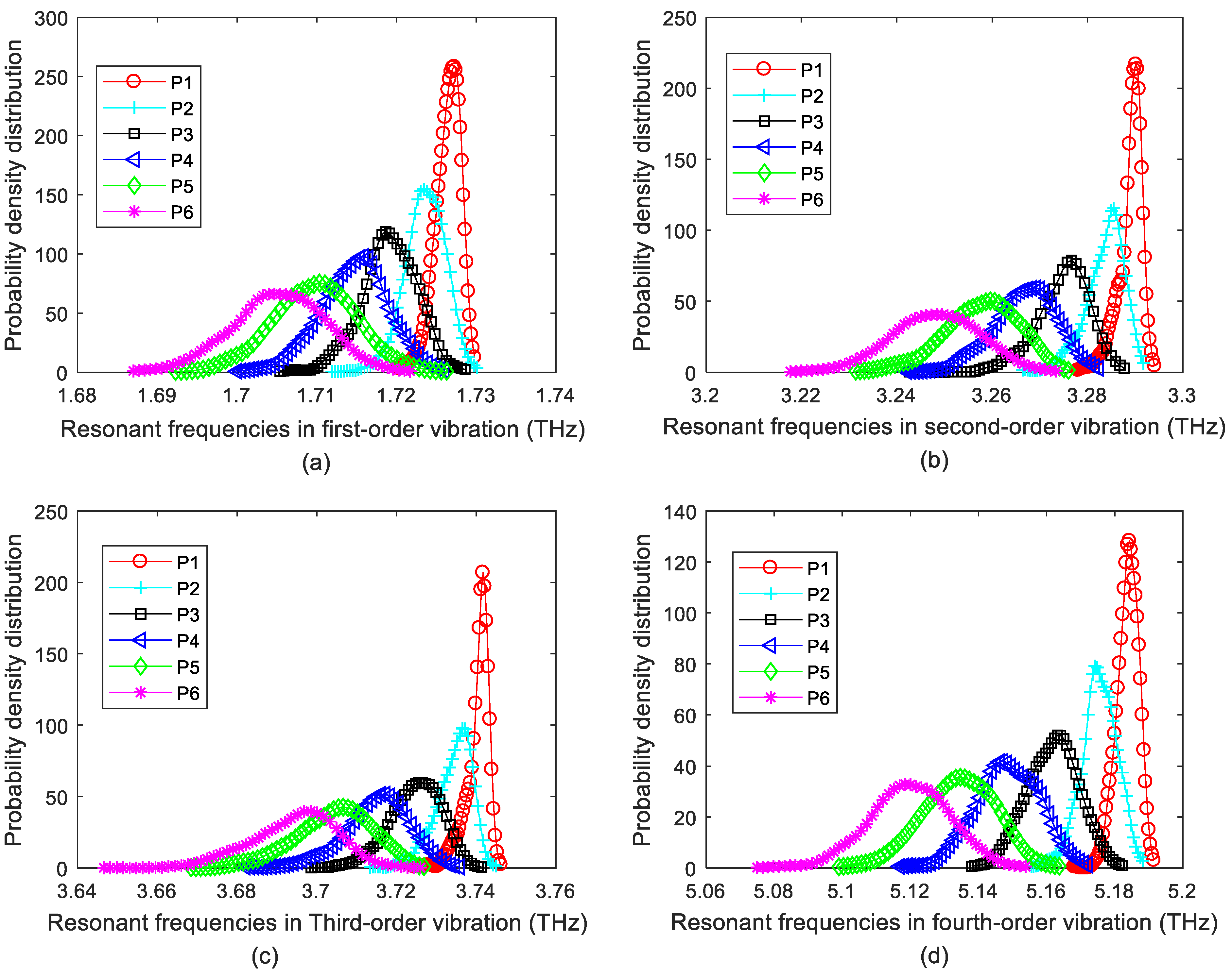
- Probability density distributions of resonant frequencies caused by random distributed atomic vacancy defects are not as regular as the Gaussian or Weibull distribution.
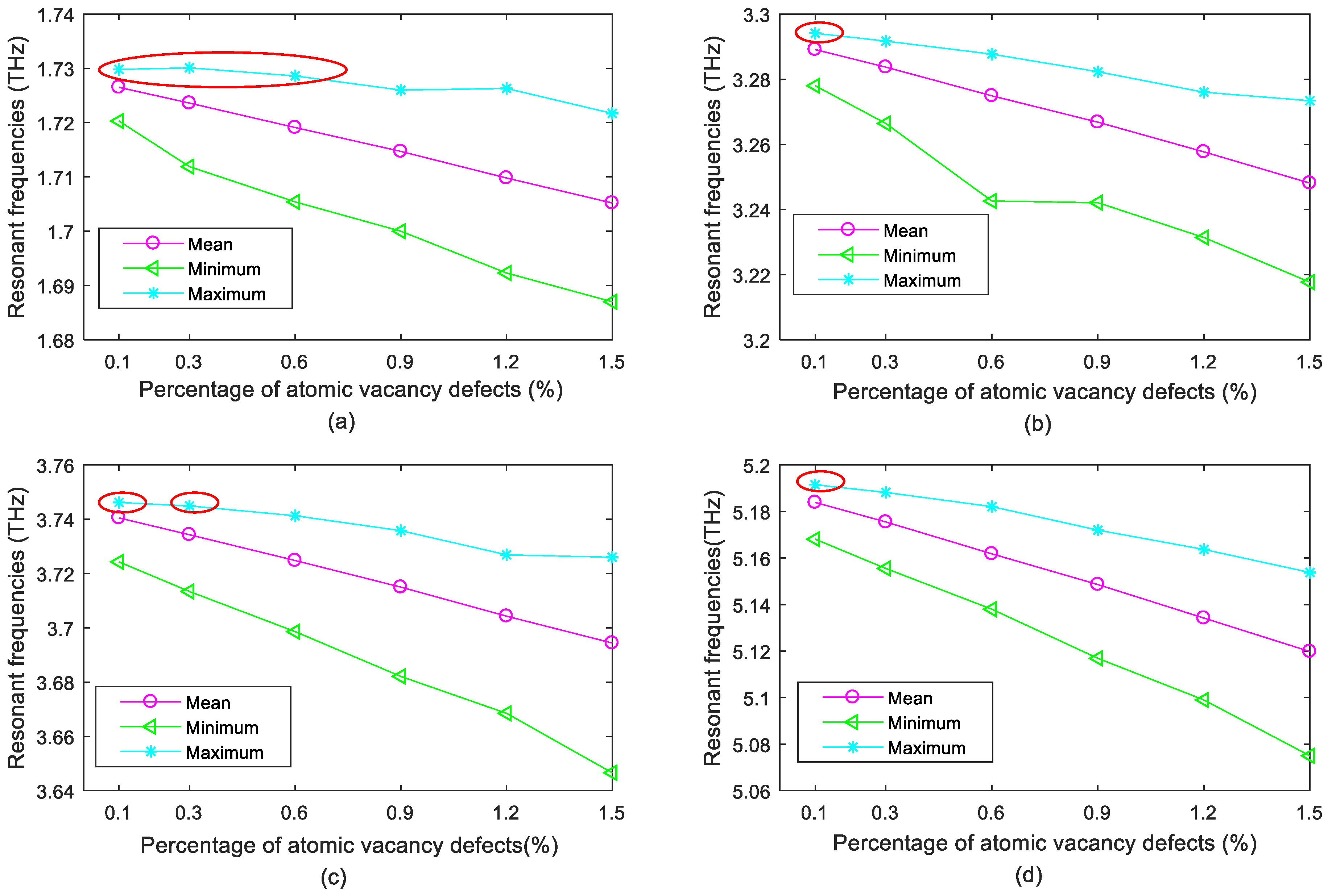
- Resonant frequencies can be amplified by the introduction of appropriate atomic vacancy defects in pristine graphene.
- Porous graphene has a stronger capacity to reduce fluctuations and deviations in low-order vibration modes than in high-order vibration modes.
- The porosities in graphene not only ensures a more solid robustness in the reduction of resonant frequencies, but also can result in stronger possible enhancement effects.
- The impacts of atomic vacancy defects are more concentrated in the local scope.
Author Contributions
Funding
Conflicts of Interest
References
- Novoselov, K.S.; Geim, A.K.; Morozov, S.V.; Jiang, D.; Zhang, Y.; Dubonos, S.V.; Grigorieva, I.V.; Firsov, A.A. Electric field effect in atomically thin carbon films. Science 2004, 306, 666–669. [Google Scholar] [CrossRef] [Green Version]
- Pruna, A.; Tamvakos, D.; Sgroi, M.; Pullini, D.; Nieto, E.A.; Busquets-Mataix, D. Electrocapacitance of hybrid film based on graphene oxide reduced by ascorbic ac-id. Int. J. Mater. Res. 2015, 106, 398–405. [Google Scholar] [CrossRef]
- Pullini, D.; Siong, V.; Tamvakos, D.; Ortega, B.L.; Sgroi, M.; Veca, A.; Glanz, C.; Kolaric, I.; Pruna, A. Enhancing the capacitance and active surface utilization of supercapacitor electrode by graphene nanoplatelets. Compos. Sci. Technol. 2015, 112, 16–21. [Google Scholar] [CrossRef]
- Ke, Q.; Wang, J. Graphene-based materials for supercapacitor electrodes—A review. J. Mater. 2016, 2, 37–54. [Google Scholar] [CrossRef] [Green Version]
- Cheng, Q.; Okamoto, Y.; Tamura, N.; Tsuji, M.; Maruyama, S.; Matsuo, Y. Graphene-Like-Graphite as Fast-Chargeable and High-Capacity Anode Materials for Lithium Ion Batteries. Sci. Rep. 2017, 7, 1–14. [Google Scholar] [CrossRef] [Green Version]
- Cai, X.; Lai, L.; Shen, Z.; Lin, J. Graphene and graphene-based composites as Li-ion battery electrode materials and their appli-cation in full cells. J. Mater. Chem. A 2017, 5, 15423–15446. [Google Scholar] [CrossRef]
- Sgroi, M.F.; Pullini, D.; Pruna, A.I. Lithium Polysulfide Interaction with Group III Atoms-Doped Graphene: A Computational Insight. Batteries 2020, 6, 46. [Google Scholar] [CrossRef]
- Bonilla, L.L.; Carpio, A. Theory of defect dynamics in graphene: Defect groupings and their stability. Contin. Mech. Thermodyn. 2011, 23, 337–346. [Google Scholar] [CrossRef] [Green Version]
- Kim, H.S.; Oweida, T.J.; Yingling, Y.G. Interfacial stability of graphene-based surfaces in water and organic solvents. J. Mater. Sci. 2017, 53, 5766–5776. [Google Scholar] [CrossRef]
- Ariza, M.P.; Ortiz, M.; Serrano, R. Long-term dynamic stability of discrete dislocations in graphene at finite temperature. Int. J. Fract. 2010, 166, 215–223. [Google Scholar] [CrossRef]
- Rani, P.; Jindal, V.K. Stability and electronic properties of isomers of B/N co-doped graphene. Appl. Nanosci. 2013, 4, 989–996. [Google Scholar] [CrossRef] [Green Version]
- Nayebi, P.; Zaminpayma, E.; Emami-Razavi, M. Study of electronic properties of graphene device with vacancy cluster defects: A first principles approach. Thin Solid Films 2018, 660, 521–528. [Google Scholar] [CrossRef]
- Li, T.; Yarmoff, J.A. Defect-induced oxygen adsorption on graphene films. Surf. Sci. 2018, 675, 70–77. [Google Scholar] [CrossRef] [Green Version]
- Araujo, E.N.D.; Brant, J.C.; Archanjo, B.S.; Medeiros-Ribeiro, G.; Alves, E.S. Quantum corrections to conductivity in graphene with vacancies. Phys. E Low Dimens. Syst. Nanostruct. 2018, 100, 40–44. [Google Scholar] [CrossRef]
- Son, J.; Choi, M.; Choi, H.; Kim, S.J.; Kim, S.; Lee, K.-R.; Vantasin, S.; Tanabe, I.; Cha, J.; Ozaki, Y.; et al. Structural evolution of graphene in air at the electrical breakdown limit. Carbon 2016, 99, 466–471. [Google Scholar] [CrossRef]
- Okada, T.; Inoue, K.Y.; Kalita, G.; Tanemura, M.; Matsue, T.; Meyyappan, M.; Samukawa, S. Bonding state and defects of nitrogen-doped graphene in oxygen reduction reaction. Chem. Phys. Lett. 2016, 665, 117–120. [Google Scholar] [CrossRef]
- Geim, A.K. Graphene: Status and Prospects. Science 2009, 324, 1530–1534. [Google Scholar] [CrossRef] [PubMed] [Green Version]
- Grantab, R.; Shenoy, V.B.; Ruoff, R.S. Anomalous Strength Characteristics of Tilt Grain Boundaries in Graphene. Science 2010, 330, 946–948. [Google Scholar] [CrossRef] [PubMed] [Green Version]
- Terdalkar, S.S.; Huang, S.; Yuan, H.; Rencis, J.J.; Zhu, T.; Zhang, S. Nanoscale fracture in graphene. Chem. Phys. Lett. 2010, 494, 218–222. [Google Scholar] [CrossRef]
- Tozzini, V.; Pellegrini, V. Reversible Hydrogen Storage by Controlled Buckling of Graphene Layers. J. Phys. Chem. C 2011, 115, 25523–25528. [Google Scholar] [CrossRef] [Green Version]
- Roszak, R.; Firlej, L.; Roszak, S.; Pfeifer, P.; Kuchta, B. Hydrogen storage by adsorption in porous materials: Is it possible? Colloids Surf. A Physicochem. Eng. Asp. 2016, 496, 69–76. [Google Scholar] [CrossRef]
- Yadav, S.; Zhu, Z.; Singh, C.V. Defect engineering of graphene for effective hydrogen storage. Int. J. Hydrogen Energy 2014, 39, 4981–4995. [Google Scholar] [CrossRef]
- Hinchet, R.; Khan, U.; Falconi, C.; Kim, S.-W. Piezoelectric properties in two-dimensional materials: Simulations and experiments. Mater. Today 2018, 21, 611–630. [Google Scholar] [CrossRef]
- Kundalwal, S.I.; Meguid, S.A.; Weng, G.J. Strain gradient polarization in graphene. Carbon 2017, 117, 462–472. [Google Scholar] [CrossRef]
- Lee, C.; Wei, X.; Kysar, J.W.; Hone, J. Measurement of the elastic properties and intrinsic strength of monolayer graphene. Science 2008, 321, 385–388. [Google Scholar] [CrossRef]
- Eckmann, A.; Felten, A.; Mishchenko, A.; Britnell, L.; Krupke, R.; Novoselov, K.S.; Casiraghi, C. Probing the Nature of Defects in Graphene by Raman Spectroscopy. Nano Lett. 2012, 12, 3925–3930. [Google Scholar] [CrossRef] [Green Version]
- Shi, J.; Chu, L.; Braun, R. A kriging surrogate model for uncertainty analysis of graphene based on a finite element method. Int. J. Mol. Sci. 2019, 20, 2355. [Google Scholar] [CrossRef] [PubMed] [Green Version]
- Qin, H.; Sun, Y.; Liu, J.Z.; Liu, Y. Mechanical properties of wrinkled graphene generated by topological defects. Carbon 2016, 108, 204–214. [Google Scholar] [CrossRef]
- Chu, L.; Shi, J.; Ben, S. Buckling Analysis of Vacancy-Defected Graphene Sheets by the Stochastic Finite Element Method. Materials 2018, 11, 1545. [Google Scholar] [CrossRef] [Green Version]
- Deng, S.; Berry, V. Wrinkled, rippled and crumpled graphene: An overview of formation mechanism, electronic properties, and applications. Mater. Today 2016, 19, 197–212. [Google Scholar] [CrossRef]
- Zandiatashbar, A.; Lee, G.-H.; An, S.J.; Lee, S.; Mathew, N.; Terrones, M.; Hayashi, T.; Picu, C.R.; Hone, J.; Koratkar, N. Effect of defects on the intrinsic strength and stiffness of graphene. Nat. Commun. 2014, 5, 3186. [Google Scholar] [CrossRef]
- Chu, L.; Shi, J.; De Cursi, E.S.; Xu, X.; Qin, Y.; Xiang, H. Monte Carlo-Based Finite Element Method for the Study of Randomly Distributed Vacancy Defects in Graphene Sheets. J. Nanomater. 2018, 2018, 3037063. [Google Scholar] [CrossRef] [Green Version]
- Ferrari, A.C.; Meyer, J.C.; Scardaci, V.; Casiraghi, C.; Lazzeri, M.; Mauri, F.; Piscanec, S.; Jiang, D.; Novoselov, K.S.; Roth, S.; et al. Raman Spectrum of Graphene and Graphene Layers. Phys. Rev. Lett. 2006, 97, 187401. [Google Scholar] [CrossRef] [PubMed] [Green Version]
- Mendez, J.P.; Ariza, M.P. Harmonic model of graphene based on a tight binding interatomic potential. J. Mech. Phys. Solids 2016, 93, 198–223. [Google Scholar] [CrossRef]
- De Oliveira Neto, P.H.; Van Voorhis, T. Dynamics of charge quasiparticles generation in armchair graphene nanoribbons. Carbon 2018, 132, 352–358. [Google Scholar] [CrossRef]
- Sinitsa, A.S.; Lebedeva, I.V.; Popov, A.M.; Knizhnik, A.A. Long triple carbon chains formation by heat treatment of graphene nanoribbon: Mo-lecular dynamics study with revised Brenner potential. Carbon 2018, 140, 543–556. [Google Scholar] [CrossRef] [Green Version]
- Özkaya, S.; Blaisten-Barojas, E. Polypyrrole on graphene: A density functional theory study. Surf. Sci. 2018, 674, 1–5. [Google Scholar] [CrossRef]
- Maschio, L.; Lorenz, M.; Pullini, D.; Sgroi, M.; Civalleri, B. The unique Raman fingerprint of boron nitride substitution patterns in gra-phene. Phys. Chem. Chem. Phys. 2016, 18, 20270–20275. [Google Scholar] [CrossRef] [PubMed]
- Ganji, M.D.; Sharifi, N.; Ahangari, M.G. Adsorption of H2S molecules on non-carbonic and decorated carbonic graphenes: A van der Waals density functional study. Comput. Mater. Sci. 2014, 92, 127–134. [Google Scholar] [CrossRef]
- Tsai, J.L.; Tu, J.F. Characterizing mechanical properties of graphite using molecular dynamics simulation. Mater. Des. 2010, 31, 194–199. [Google Scholar] [CrossRef]
- Javvaji, B.; Budarapu, P.; Sutrakar, V.; Mahapatra, D.R.; Paggi, M.; Zi, G.; Rabczuk, T. Mechanical properties of Graphene: Molecular dynamics simulations correlated to continuum based scaling laws. Comput. Mater. Sci. 2016, 125, 319–327. [Google Scholar] [CrossRef] [Green Version]
- Gupta, S.; Dharamvir, K.; Jindal, V.K. Elastic moduli of single-walled carbon nanotubes and their ropes. Phys. Rev. B 2005, 72, 165428. [Google Scholar] [CrossRef]
- Sadeghzadeh, S.; Khatibi, M.M. Modal identification of single layer graphene nano sheets from ambient re-sponses using frequency domain decomposition. Eur. J. Mech. A/Solids 2017, 65, 70–78. [Google Scholar] [CrossRef]
- Kudin, K.N.; Scuseria, G.E.; Yakobson, B.I. C2F, BN, and C nanoshell elasticity from ab initio, computations. Phys. Rev. B 2001, 64, 235406. [Google Scholar] [CrossRef]
- Liu, F.; Ming, P.; Li, J. Ab initio, calculation of ideal strength and phonon instability of graphene under tension. Phys. Rev. B 2007, 76, 471–478. [Google Scholar] [CrossRef] [Green Version]
- Wei, X.; Fragneaud, B.; Marianetti, C.A.; Kysar, J.W. Nonlinear elastic behavior of graphene: Ab initio calculations to con-tinuum description. Phys. Rev. B 2009, 80, 205407. [Google Scholar] [CrossRef] [Green Version]
- Cadelano, E.; Palla, P.L.; Giordano, S.; Colombo, L. Nonlinear Elasticity of Monolayer Graphene. Phys. Rev. Lett. 2009, 102, 235502. [Google Scholar] [CrossRef] [Green Version]
- Zhou, L.; Wang, Y.; Cao, G. Elastic properties of monolayer graphene with different chiralities. J. Phys. Condens. Matter 2013, 25, 125302. [Google Scholar] [CrossRef]
- Reddy, C.D.; Rajendran, S.; Liew, K.M. Equilibrium configuration and continuum elastic properties of finite sized graphene. Nanotechnology 2006, 17, 864–870. [Google Scholar] [CrossRef]
- Chu, L.; Shi, J.; Souza de Cursi, E. Vibration Analysis of Vacancy Defected Graphene Sheets by Monte Carlo Based Finite Element Method. Nanomaterials 2018, 8, 489. [Google Scholar] [CrossRef] [Green Version]
- Belytschko, T.; Xiao, S.P.; Schatz, G.C.; Ruoff, R.S. Atomistic simulations of nanotube fracture. Phys. Rev. B 2002, 65, 235430. [Google Scholar] [CrossRef] [Green Version]


| Per (%) | Mode | Mean (THz) | Minimum (THz) | Maximum (THz) | Variance |
|---|---|---|---|---|---|
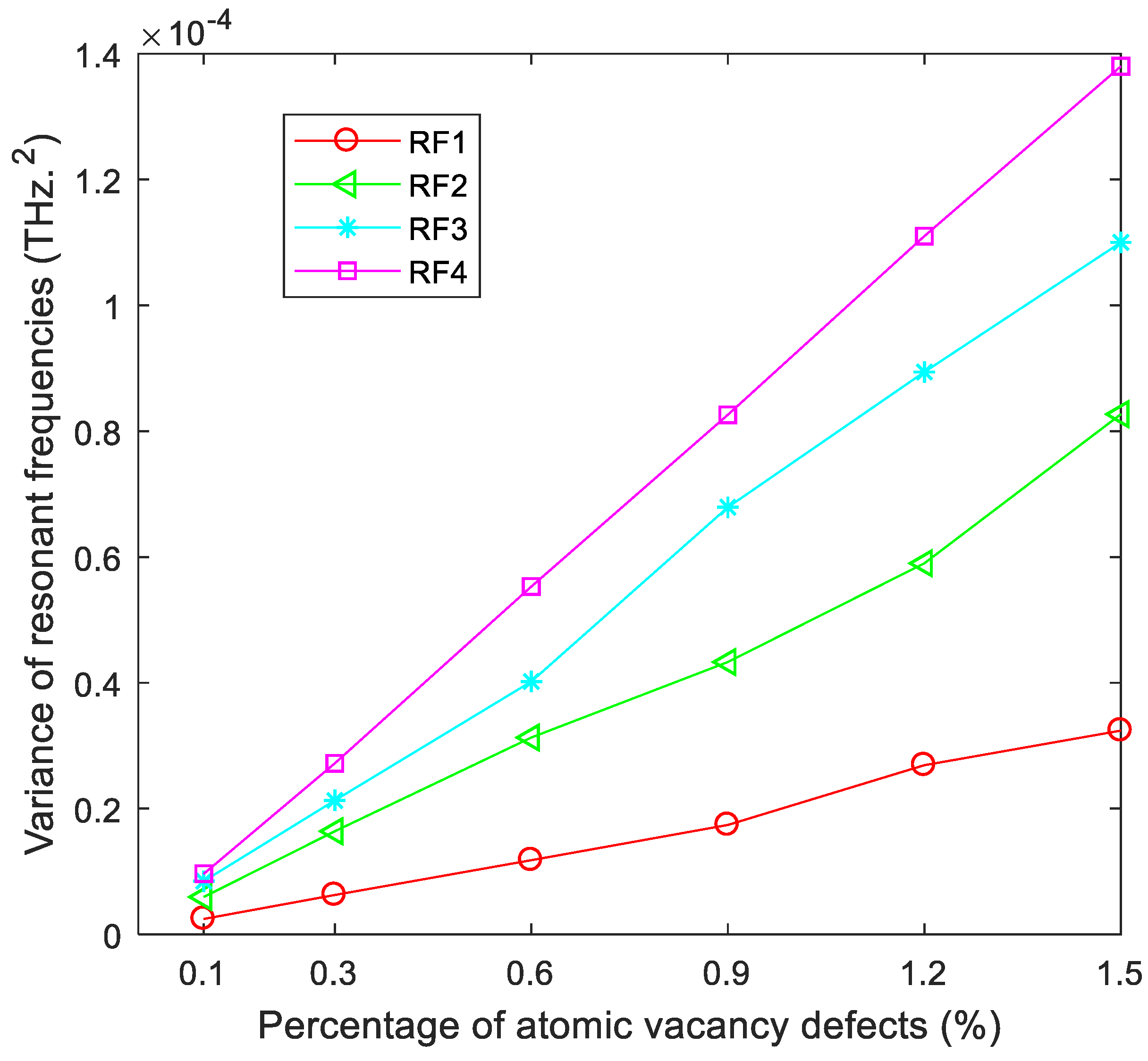
| 0.1 | 1 | 1.7265 | 1.7203 | 1.7298 | 2.46 × 10⁻⁶ |
| 2 | 3.2891 | 3.2780 | 3.2941 | 5.95 × 10⁻⁶ | |
| 3 | 3.7405 | 3.7243 | 3.7462 | 8.47 × 10⁻⁶ | |
| 4 | 5.1839 | 5.1681 | 5.1915 | 9.64 × 10⁻⁶ | |
| 0.3 | 1 | 1.7236 | 1.7119 | 1.7301 | 6.27 × 10⁻⁶ |
| 2 | 3.2837 | 3.2664 | 3.2917 | 1.64 × 10⁻⁵ | |
| 3 | 3.7343 | 3.7134 | 3.7449 | 2.13 × 10⁻⁵ | |
| 4 | 5.1755 | 5.1555 | 5.1882 | 2.72 × 10⁻⁵ | |
| 0.6 | 1 | 1.7191 | 1.7054 | 1.7286 | 1.18 × 10⁻⁵ |
| 2 | 3.2749 | 3.2426 | 3.2877 | 3.13 × 10⁻⁵ | |
| 3 | 3.7248 | 3.6986 | 3.7413 | 4.02 × 10⁻⁵ | |
| 4 | 5.1618 | 5.1380 | 5.1821 | 5.53 × 10⁻⁵ | |
| 0.9 | 1 | 1.7147 | 1.7000 | 1.7260 | 1.74 × 10⁻⁵ |
| 2 | 3.2668 | 3.2421 | 3.2823 | 4.33 × 10⁻⁵ | |
| 3 | 3.7150 | 3.6821 | 3.7358 | 6.79 × 10⁻⁵ | |
| 4 | 5.1486 | 5.1169 | 5.1720 | 8.26 × 10⁻⁵ | |
| 1.2 | 1 | 1.7098 | 1.6923 | 1.7263 | 2.69 × 10⁻⁵ |
| 2 | 3.2577 | 3.2314 | 3.2760 | 5.90 × 10⁻⁵ | |
| 3 | 3.7043 | 3.6685 | 3.7269 | 8.94 × 10⁻⁵ | |
| 4 | 5.1342 | 5.0990 | 5.1637 | 1.11 × 10⁻⁴ | |
| 1.5 | 1 | 1.7052 | 1.6870 | 1.7217 | 3.24 × 10⁻⁵ |
| 2 | 3.2481 | 3.2177 | 3.2734 | 8.27 × 10⁻⁵ | |
| 3 | 3.6944 | 3.6466 | 3.7260 | 1.10 × 10⁻⁴ | |
| 4 | 5.1198 | 5.0750 | 5.1538 | 1.38 × 10⁻⁴ |
| Per (%) | Mode | Mean (THz) | Minimum (THz) | Maximum (THz) | Variance |
|---|---|---|---|---|---|
| 0.1 | 1 | 1.7267 | 1.7220 | 1.7286 | 1.04 × 10⁻⁶ |
| 2 | 3.2896 | 3.2783 | 3.2936 | 4.40 × 10⁻⁶ | |
| 3 | 3.7408 | 3.7304 | 3.7476 | 5.70 × 10⁻⁶ | |
| 4 | 5.1847 | 5.1766 | 5.1893 | 4.58 × 10⁻⁶ | |
| 0.3 | 1 | 1.7242 | 1.7166 | 1.7286 | 3.01 × 10⁻⁶ |
| 2 | 3.2846 | 3.2664 | 3.2923 | 1.04 × 10⁻⁵ | |
| 3 | 3.7353 | 3.7140 | 3.7450 | 1.77 × 10⁻⁵ | |
| 4 | 5.1765 | 5.1637 | 5.1851 | 1.30 × 10⁻⁵ | |
| 0.6 | 1 | 1.7199 | 1.7108 | 1.7269 | 5.54 × 10⁻⁶ |
| 2 | 3.2766 | 3.2579 | 3.2873 | 2.22 × 10⁻⁵ | |
| 3 | 3.7260 | 3.7010 | 3.7422 | 3.47 × 10⁻⁵ | |
| 4 | 5.1640 | 5.1323 | 5.1776 | 2.93 × 10⁻⁵ | |
| 0.9 | 1 | 1.7153 | 1.7038 | 1.7229 | 9.52 × 10⁻⁶ |
| 2 | 3.2680 | 3.2480 | 3.2833 | 3.46 × 10⁻⁵ | |
| 3 | 3.7160 | 3.6912 | 3.7363 | 5.70 × 10⁻⁵ | |
| 4 | 5.1496 | 5.1242 | 5.1691 | 4.73 × 10⁻⁵ | |
| 1.2 | 1 | 1.7110 | 1.6962 | 1.7213 | 1.41 × 10⁻⁵ |
| 2 | 3.2593 | 3.2323 | 3.2769 | 4.72 × 10⁻⁵ | |
| 3 | 3.7068 | 3.6723 | 3.7342 | 8.11 × 10⁻⁵ | |
| 4 | 5.1345 | 5.1003 | 5.1576 | 6.88 × 10⁻⁵ | |
| 1.5 | 1 | 1.7017 | 0 | 1.7174 | 5.83 × 10⁻³ |
| 2 | 3.2425 | 0 | 3.2706 | 2.12 × 10⁻² | |
| 3 | 3.6866 | 0 | 3.7233 | 2.74 × 10⁻² | |
| 4 | 5.1063 | 0 | 5.1431 | 5.24 × 10⁻² |
Publisher’s Note: MDPI stays neutral with regard to jurisdictional claims in published maps and institutional affiliations. |
© 2021 by the authors. Licensee MDPI, Basel, Switzerland. This article is an open access article distributed under the terms and conditions of the Creative Commons Attribution (CC BY) license (https://creativecommons.org/licenses/by/4.0/).
Share and Cite
Chu, L.; Shi, J.; Yu, Y.; Souza De Cursi, E. The Effects of Random Porosities in Resonant Frequencies of Graphene Based on the Monte Carlo Stochastic Finite Element Model. Int. J. Mol. Sci. 2021, 22, 4814. https://doi.org/10.3390/ijms22094814
Chu L, Shi J, Yu Y, Souza De Cursi E. The Effects of Random Porosities in Resonant Frequencies of Graphene Based on the Monte Carlo Stochastic Finite Element Model. International Journal of Molecular Sciences. 2021; 22(9):4814. https://doi.org/10.3390/ijms22094814
Chicago/Turabian StyleChu, Liu, Jiajia Shi, Yue Yu, and Eduardo Souza De Cursi. 2021. "The Effects of Random Porosities in Resonant Frequencies of Graphene Based on the Monte Carlo Stochastic Finite Element Model" International Journal of Molecular Sciences 22, no. 9: 4814. https://doi.org/10.3390/ijms22094814