
Differential Entropy-Based Fault-Detection Mechanism for Power-Constrained Networked Control Systems

Departamento de Ingeniería Eléctrica, Universidad de Concepción, Concepción 4070409, Chile
Entropy 2024, 26(3), 259; https://doi.org/10.3390/e26030259
Submission received: 17 January 2024
/
Revised: 4 March 2024
/
Accepted: 12 March 2024
/
Published: 14 March 2024
(This article belongs to the Special Issue The Application of Information Theory in Fault Detection and Diagnosis)
Abstract
:In this work, we consider the design of power-constrained networked control systems (NCSs) and a differential entropy-based fault-detection mechanism. For the NCS design of the control loop, we consider faults in the plant gain and unstable plant pole locations, either due to natural causes or malicious intent. Since the power-constrained approach utilized in the NCS design is a stationary approach, we then discuss the finite-time approximation of the power constraints for the relevant control loop signals. The network under study is formed by two additive white Gaussian noise (AWGN) channels located on the direct and feedback paths of the closed control loop. The finite-time approximation of the controller output signal allows us to estimate its differential entropy, which is used in our proposed fault-detection mechanism. After fault detection, we propose a fault-identification mechanism that is capable of correctly discriminating faults. Finally, we discuss the extension of the contributions developed here to future research directions, such as fault recovery and control resilience.
1. Introduction
Control theory developed mainly after World War II. The ideas proposed in this research area are typically related to proportional-integral-differential (PID) control design, state feedback optimal control, optimal observers, and model predictive control (MPC); see [1]. At the turn of the twenty-first century and soon thereafter, the next step was taken under the networked control system (NCS) paradigm, which has evolved into multiagent consensus control [2], cybersecurity [3,4], and data-driven control [5]. Since then, control theorists and control practitioners have remained highly active in this research area, such as by combining control and information theories [6,7] or linear optimal control and communication theory; examples include [8,9,10]. The last few years have also seen an increase in event-triggered NCS solutions [11,12,13], that is, asynchronous control closed-loop solutions, which aim to increase the efficiency of specifically limited communication resources while achieving a set of given objectives (stability, performance, robustness, or a combination of these). These and other NCS results are the foundation of better control.
An approach to NCS introduced early on by [9] imposes a power constraint, , on the channel input power and then characterizes the channel model by its channel signal-to-noise ratio (SNR). The proposed SNR approach is then used to study the design constraints on closed-loop stability, especially for cases in which the controlled plant model under analysis is unstable. The SNR limitations presented in [9], which are fundamental in nature, deal with unstable single-input–single-output (SISO) LTI plant models, characterizing the initial bound on the channel SNR required to achieve feedback-loop stability for a single-channel model in the closed loop. A mean square analysis to address the probabilistic nature of the communication network was also used, in a different context of synchronization, in [14]. An NCS extension of the setup proposed in [9] is presented in Figure 1; in this paper, we consider a memoryless additive white Gaussian noise (AWGN) communication channel for the communication network, which operates simultaneously over two paths: the direct path between the controller and the plant and the feedback path between the plant and the controller.
A vast amount of literature also exists on the topic of fault detection and diagnostics, including many published books [15,16,17,18,19] and review articles [20,21]. A fault occurs when there is an anomalous behavior, either by chance or maliciously induced, in a physical plant; it is then important to detect, identify, and if possible recover from this fault. There are different formulations for the problems of fault detection and fault identification for linear time-invariant (LTI) models, which can be roughly categorized as approximate (such as synthesizing fault-detection filters subject to noise) and exact formulations (such as the null-space method).
The variability inherent in NCSs due to the inclusion of stochastic processes in the communication of relevant closed-loop signals might also be caused by variations in the plant model parameters. These parameter variations can be interpreted as faults; thus, a fault mechanism is needed that can detect these changes, identify them, and, through the residuals (see Figure 1), identify the new faulty parameter values to then adapt the controller’s design to achieve fully fault-tolerant closed loop control. A two-part survey on fault diagnosis and fault-tolerant techniques in control can be found in [22,23]. In contrast, the author of [24] offers a complete survey on the topics of fault detection and fault-tolerant control for NCSs. Another survey on fault diagnosis for NCSs can be found in [25], which aims to reduce performance degradation due to communication features. In [26], a fault-detection filter subject to limited transmission through a network with time-varying latency and fading was successfully designed. A Bayesian approach was used instead in [27] for NCS fault diagnosis in an irrigation canal application, while in [28] the authors used a Markov jumping linear system (MJLS) approach for the design of a residual generator. NCS robust fault-tolerant control is also an alternative, which was subsequently considered, for example, in [29]; faults were modeled as MJLSs with incomplete transition probabilities, and LMI-based sufficient conditions were then used to ensure stability. Task allocation in a multiagent setting was presented in [30] to ensure fault tolerance through cooperation between healthy and faulty agents instead of focusing on recovering nominal performance; see also [31]. Finally, a nonlinear MPC solution subject to random network delays and packet dropout was used for fault-tolerant design control in [32].
Our first contribution is the optimal design of the control loop for a first-order unstable plant model, which applies generally due to the nature of the NCS setup. The optimal controller minimizes the sum of the powers for the network input signals (also the controller output) and (also the plant model output) in the steady state; see Figure 1. Our second contribution is a fault-detection mechanism based on the estimation of the differential entropy of the controller output signal u, as shown in Figure 1. Our third contribution is a fault-identification mechanism for the value of the plant model gain and unstable poles, once a fault has been detected, based on the controller output signal u and the received output signal . We present a simulated example to illustrate these contributions.
This paper is organized as follows. Section 2 presents the general assumptions, introducing the plant and AWGN channel models. Here, we also present the definition of the power of a signal in the steady state. In Section 3, we propose the optimal controller design for the power-constrained NCS control loop. In Section 4, we define the finite-time power estimation and the power constraint-based fault-detection criterion. Section 5 introduces the proposed fault-identification mechanism. In Section 6, we demonstrate the use of both the fault-detection and fault-identification mechanisms based on a simulation example. Finally, in Section 7, we summarize the present work and possible future research avenues.
2. Preliminaries
2.1. Plant, Channel, and Network Models
We next give the descriptions of the plant, channel, and network models under study.
- Plant Model: The plant model, , can be described by a general model given bywhere , , and is a stable, minimum-phase transfer function (i.e., all its poles and zeros are inside the unit circle).
- Channel Models: The AWGN channel model is described by a channel input power constraint, P, and an identically independently distributed additive Gaussian noise process, n, with zero mean and variance, .
- Network Model: We define the network as two AWGN channel models with an encoder and decoders, one of which is on the direct path between the controller and the plant models and one of which is on the feedback path between the plant and the controller models; see Figure 2. Depending on the channel location, we identify the additive noises as and , both of which are identically independently distributed additive Gaussian noise processes with zero means and variances, and , respectively. Finally, the powers of the channel input signals are denoted as and .
Furthermore, the setpoint signal, , in Figure 2 is assumed to be a constant known value.
Remark 1.
The decision to use AWGN channel models to characterize the proposed network model implies that we are considering the channel input constraints and the channel additive noises as the main network features. Other network features, such as transmission delays, quantization, and packet losses, can also be considered, but this would require the use of channel models in addition to the proposed AWGN channel model and would make the characterization of the differential entropy of the control signal, , which is the basis of the proposed fault-detection mechanism, more involved due to the effect of the closed loop.
2.2. Stationary Power of a Linear Time-Invariant System Output Signal
Definition 1.
Definition 2.
The norm of a discrete-time linear time-invariant system H is defined as
Lemma 1
(Stationary power of an LTI system output signal). For a discrete-time linear time-invariant system H with a weakly stationary stochastic process at the input, mean , and spectral density
the variance of the noise can be determined. Ref. [34] shows that if H is stable (here, it is assumed to be stable if all its poles are inside the unit circle), then
and the steady-state power of the output signal is then
Proof.
Since is a weakly stationary stochastic process and H is stable, s is also a weakly stationary stochastic process. If we define , where is a weakly stationary stochastic process with zero mean, then we have
Since, by its definition, the covariance function of is equal to the covariance function of s, and because the power spectral density is the Fourier transform of the covariance function, we have that . As we take the limit , we obtain
In the next section, we use the introduced assumptions and Lemma 1 to propose the design of the NCS control loop in Figure 2.
3. Networked Control System Design
We start this section with the following lemma, which references a result from [35]; from this lemma, we begin to construct our optimal controller design proposal.
Lemma 2
(sum of convex functions). Let be given convex functions and be given positive scalars. Then, the function
is also a convex function.
Proof.
See [35]. □
We continue by establishing the working choices for the encoder and decoder blocks in Figure 2. The presence of these blocks is intrinsic to the NCS setup, and it is one of the reasons these types of systems require an extension, not just an application, of classic control theory results.
Lemma 3
(Encoder and decoder design). The encoder and decoder blocks in Figure 2 for the subsequent NCS design are selected as
where is the stable, minimum-phase part of the proposed plant model; see Section 2.1.
Remark 2.
We observe that, by using Lemma 3 in Figure 2, we can focus entirely on the first-order unstable part of the plant model.
In the next lemma, we introduce some intermediate results that consider the controller, , to be a proportional controller; that is, for , which will be required for the optimal controller design .
Lemma 4
(Convexity of closed-loop squared norms). The following squared norms are convex functions of , the proportional controller:
where is the closed-loop complementary sensitivity and is the closed-loop sensitivity.
Proof.
We start this proof with the squared norm of T. For a proportional controller and the simplified plant model, , the complementary sensitivity is
The squared norm of the above transfer function is then
To obtain its critical points, we take the derivative of and solve
After grouping the powers of in the numerator, we obtain
One critical point is , but this solution is outside the region of values that ensures closed-loop stability and is thus not considered. The other critical point is . The second derivative is
Thus, , the only valid critical point, is a minimum, proving that is a convex function. Now, for , we have that
Thus, since is a convex function of , we focus on the remaining part, :
The value is a critical point with a multiplicity of three, but again, it is outside the range of values required for closed-loop stability for . The other two potential solutions are
but we observe that is outside the stability region. The second derivative at yields
Simplifying, we obtain
Therefore, we determine that the numerator and thus the overall second partial derivative at are positive and that the only critical point value, , is a minimum, which proves that is a convex function of in the stability region; through Lemma 2, is also a convex function of in the stability region. Finally, we focus on the term . For the last squared norm expression, , we have
The only critical point in this case is given by , which lies inside the stability region for the closed loop; when replaced in the second partial derivative, it results in
Thus, the critical point, , is a minimum, and the function is convex in the stability region for the closed loop; this concludes the proof. □
We next use the results just obtained to show the convexity, in terms of the proportional controller, of the power expression for the NCS input signals u and y; see Figure 2.
Lemma 5
(Channel input powers). For the setup depicted in Figure 2 with , the channel input powers are
and they are both convex functions of , the proportional controller.
We are now ready to use all the previous intermediate results to present the optimal design of the proportional controller, which minimizes the sum of the channel input powers.
Proof.
According to Figure 2 and Lemma 3, the signals at the respective channel inputs are
We then apply Lemma 1 for and for and obtain the expressions in Equation (9). Finally, since all the squared elements of Equation (9) are convex functions of as in Lemma 4, together with Lemma 2, it is shown that the channel input powers in Equation (9) are convex functions of , which concludes this proof. □
Theorem 1
(NCS controller design). The proportional controller, , is designed so that
with , and its optimal value is the unique solution, in the stability region for the closed loop, of the following polynomial:
Proof.
From Lemma 5, we have that
According to Lemma 2, this is a convex function of , thus characterizing the critical point of the above functional results in obtaining the optimal that minimizes the linear combination of channel input powers. We then take the partial derivative of , which results in the polynomial , with coefficients defined as in (11). Since the proposed functional is convex in , there is only one critical point in the stability region for the closed loop, which concludes this proof. □
Remark 3.
If the plant pole ρ (see (1)) is stable, that is, if , then the minimal channel input powers and will be zero, and the optimal controller from Theorem 1 will also then be equal to zero, nevertheless resulting in a stable closed loop (although it is technically open if the controller is zero). The fault-detection and fault-identification mechanisms described in the next sections will be applicable as long as a non-zero suboptimal controller is in place for to effectively close the loop.
Remark 4.
Due to the standing assumptions regarding , the choice of in Figure 2, and the relationship between stationary power and signal variance, we have that the NCS controller design proposed in Theorem 1, which minimizes the network input power, can also be interpreted as a minimal-input-entropy controller design.
The optimal controller design from Theorem 1 results in a stable closed loop, and we now wish to extend its analysis to the case with faults on the two main parameters involved in the optimal controller design, namely, the gain, , and the plant unstable pole, . We obtain two contributions: a fault-detection mechanism and a fault-identification mechanism. Therefore, we continue by presenting the proposed fault-detection mechanism in the next section.
4. Fault-Detection Mechanism
The signal u is assumed to be available because it is the result of signal processing through the controller, as shown in Figure 1. On the other hand, the availability of the signal requires the assumption of an added sensor at the output of the AWGN channel over the feedback path. Moreover, due to the presence of the channel additive processes and , we cannot consider the instant values of the relevant signals u and , as shown in Figure 1, as representative values. We therefore address this issue by using the average estimates of u and instead, as shown in the next lemma.
Lemma 6
(Finite time estimate). The averaged signal is obtained as
where L satisfies
for a user-defined tolerance value ϵ.
Proof.
Lemma 5 shows that
In a stationary state, we then have that , as defined in (12), will approach as and since is a constant value, which shows that there will always be a suitable finite value of L for any given choice of tolerance , which concludes this proof. □
Remark 5.
The use of the previous lemma extends in exactly the same way for signal , for which represents the L average. However, such a signal is only required for the fault-identification mechanism that we propose in the next section.
Remark 6.
The application of Lemma 6 is based on a Monte Carlo simulation of the NCS-designed control closed loop in steady state with no faults. The selected value of L, through the choice of ϵ, will be a user-selected trade-off between the successful rejection of the noise processes (the larger the L value is, the better) and the responsiveness to the presence of faults (the smaller the L value is, the better).
We now present our proposed fault-detection mechanism in the following theorem.
Theorem 2
(fault-detection mechanism). Given the setup in Figure 2 for the NCS defined by Lemma 3, with the controller designed as in Theorem 1, the fault flag signal, , is defined as
where
is the estimated differential entropy of the signal , with the time estimate defined in Lemma 6 and defined as
Additionally,
is the theoretical differential entropy of the signal in the steady state when no fault is present. The fault level, δ, is user defined, and it is selected as , which is twice the standard deviation of the estimated differential entropy of when no fault is present.
Proof.
Remark 7.
We observe that the selection of δ in Theorem 2 is a compromise between false negative errors (not detecting a fault when one is present) and false positive errors (detecting a fault when one is not present). If the selected δ value is smaller, then more false positive errors will be detected. If the selected δ value is greater, then more false negative errors will be detected.
Remark 8.
The use of differential entropy for the proposed fault-detection mechanism is motivated by the presence of the AWGN channel and is also a reasonable choice because it introduces a logarithmic scale (base 2 in this case) for the channel input variance, which can otherwise report very large excursions when subjected to faults, as we will observe in the following sections. Moreover, if we select in Theorem 1 for the NCS controller design, we can then address the minimal in (17).
After a fault has been detected by means of Theorem 2, the next step is to estimate its value, that is, to identify it. The next section focuses on this goal.
5. Fault-Identification Mechanism
The faults that the control loop might be subject to are involved in the plant model gain, , or the unstable pole . Additionally, due to the NCS nature of the proposed closed control loop in Figure 2, for the fault-identification mechanism we only stipulate that we have access to the signals u and . That is, we only stipulate access to signals on the controller side of the network (otherwise, transmission through a communication channel would be required); see Figure 1.
As a first step in identifying the detected faults, as described in the previous section, we consider the online estimation of the plant parameters and .
Lemma 7
(Plant parameter estimation). From Figure 1, assuming the online availability of signals and and a selected value of L from Lemma 6, we obtain
and the plant parameter estimates are
Proof.
We first observe that
where is the L-length finite-time estimation of the steady-state value of . From this, we obtain
On the other hand, we have
and thus
With these two intermediate results, after algebraic manipulation we obtain the estimate expressions in (19), which concludes this proof. □
We now use Lemma 7, together with the fault-detection mechanism from the previous section, to identify the fault. We provide this result in the next theorem.
Theorem 3
(fault-identification mechanism). The values of the plant fault parameters are identified as
for the plant parameter, , where is the standard deviation of the plant gain estimation when no fault is present and
for the plant parameter ρ, where is the standard deviation of the unstable plant pole estimation when no fault is present.
Proof.
Fault identification is the result of intersecting the estimated plant parameters and from Lemma 7 with the fault flag signal from Theorem 2. Whether the fault is due to , , or a change in the values of both and , the type of fault will be identified as long as the excursion in the value of the faulty parameter exceeds twice the standard deviation of the estimated parameter value when no fault is present. That is, we use the same approach proposed in Theorem 2, but now we validate the fault on either or both plant parameters. □
We have now finalized the theoretical development of this work, and we proceed in the next section to illustrate the proposed contributions through a simulation example summarizing all the previous key points.
6. Example
In this section, we develop an example to illustrate the contributions developed in the previous sections. We consider the plant model
That is, we assume for simplicity here, without loss of generality, that . The setpoint signal is , and the channel additive noise variances are selected as . The NCS proportional controller design from Theorem 1, with an equal weight to equally weight the power contribution of each channel input, results in . The plant model parameters, and thus the closed control loop, are subject to the following changes for :
For ,
We then propose a first fault on the value of starting at and lasting until 12,000, a second fault due to starting at 17,001 and lasting until 24,000, and a third and final fault due to a simultaneous change in the values of and starting at 29,001 and ending at 36,000.
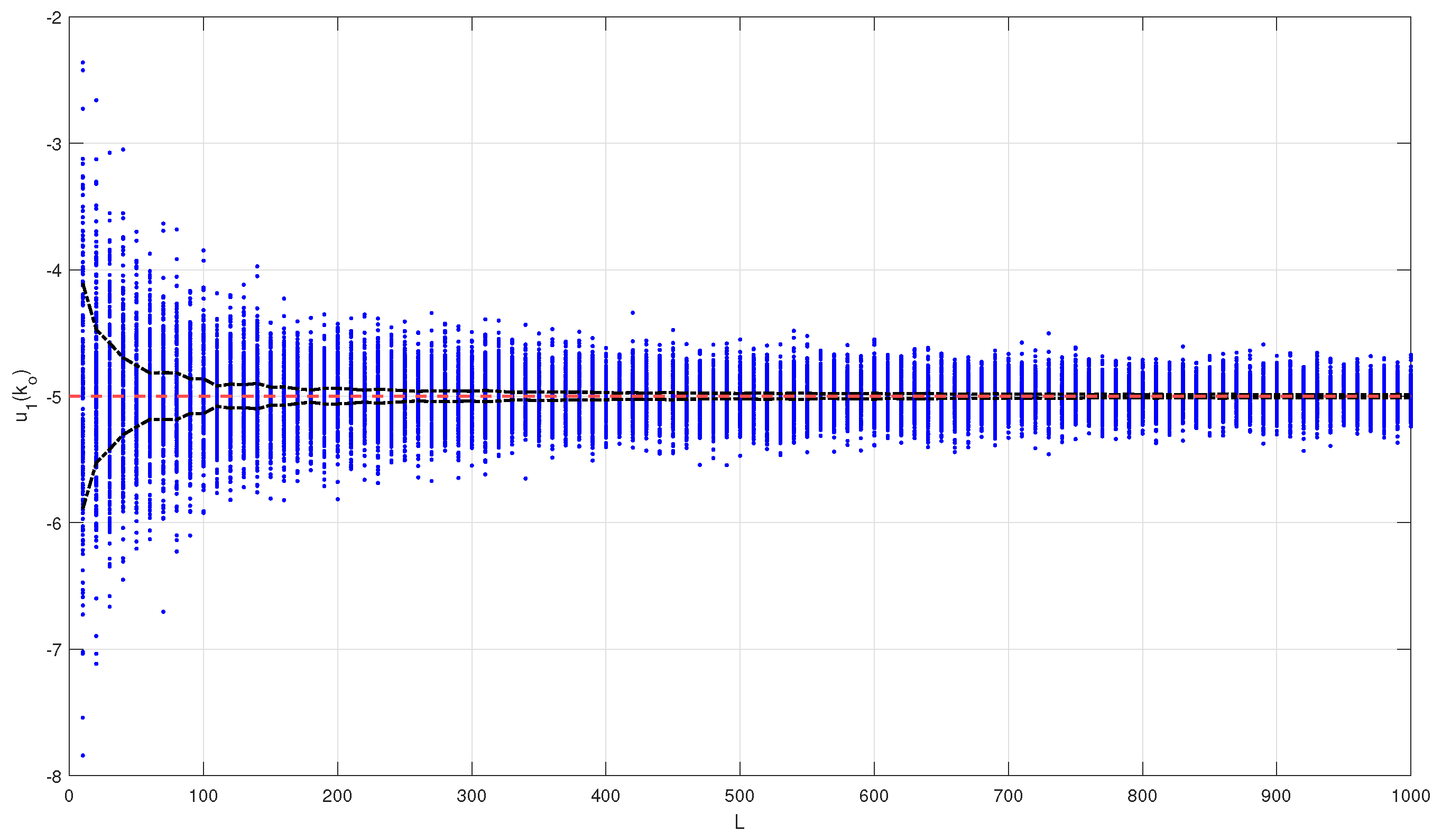
The first step is the selection of L as a compromise between the rejection of the two noise processes and responsiveness to the faults. In Figure 3, we show a Monte Carlo simulation of two hundred simulations of at for each value of L, in steps of ten. The red dashed line is the steady-state predicted value, , and the black dash-dotted lines are the variances of the two hundred simulations at each value of L around the mean value. As predicted, the variance decreases as L increases. From Figure 3, the choice of is considered a good compromise, and it is the value used in the following steps. The proposed selection is compatible with a tolerance value of .
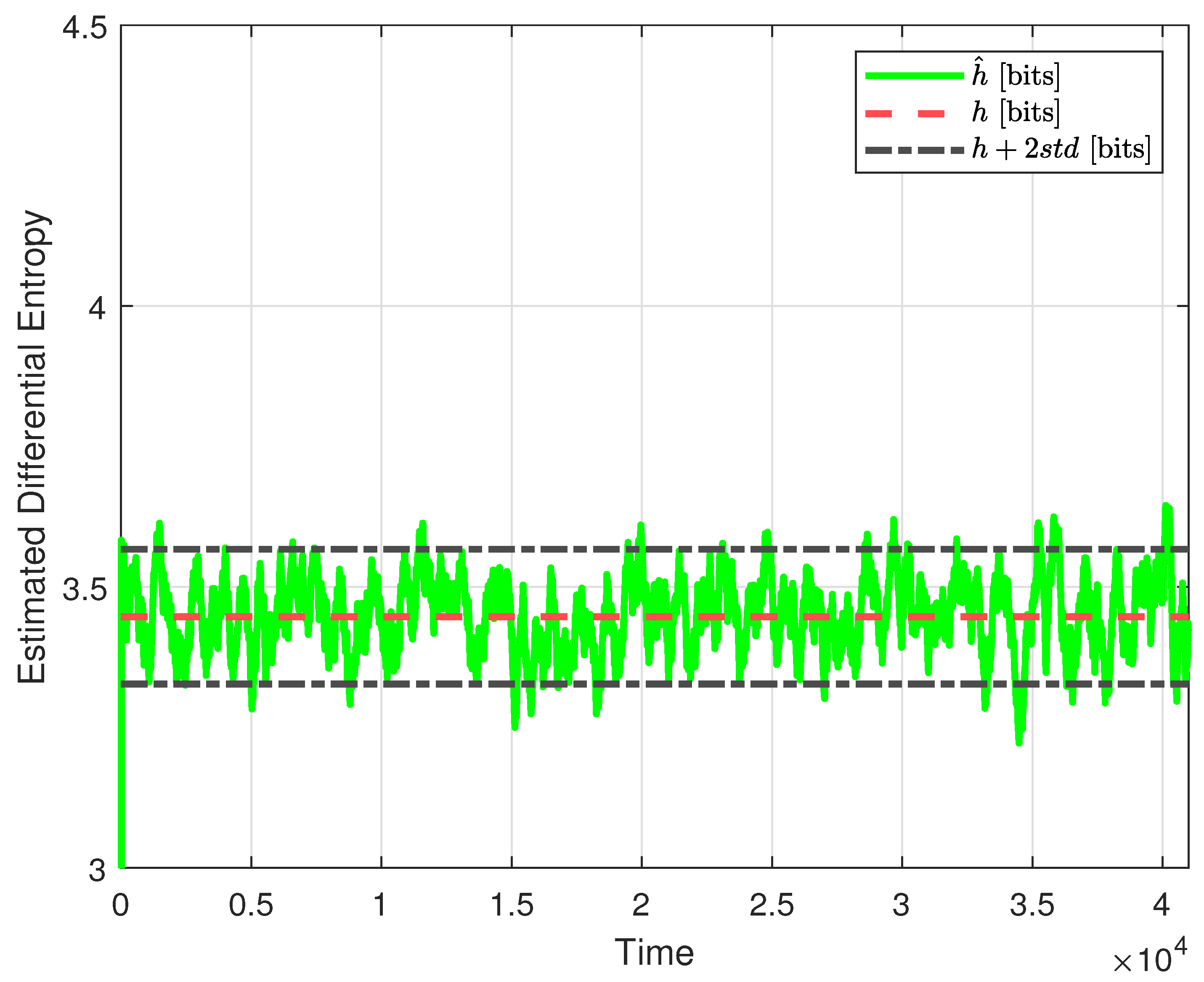
As a second step, focusing on Theorem 2, we provide the estimate (solid green line) and propose from the same figure a choice of that is twice the standard deviation of the observed , which in this case amounts to . Therefore, any increase in the estimated differential entropy, , of more than from the base value, , represented by the red dashed line in Figure 4, is registered as a fault.
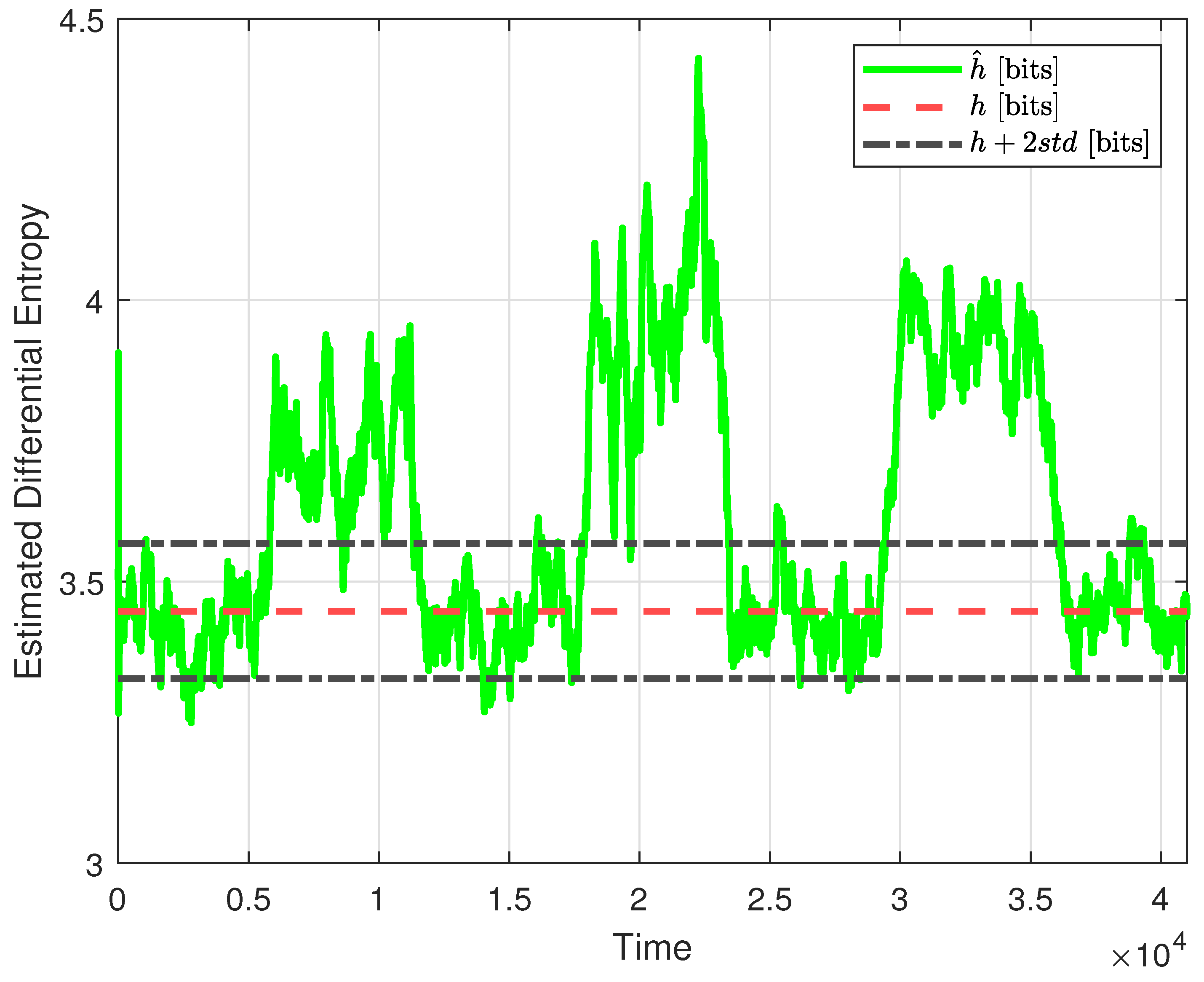
We now test the proposed fault-detection mechanism for the designed NCS closed control loop, with the faults described in (21) and (22). In Figure 5, the three proposed faults can be clearly observed. With the selected value of , there will be small instances of false negative errors for around and for around 19,600. However, no false negative errors are present for simultaneous faults and . The choice of also triggers some instances of false positive errors around , 16,000, 25,000, and 39,000. This is the expected trade-off between false positive errors and false negative errors for any fault-detection mechanism.
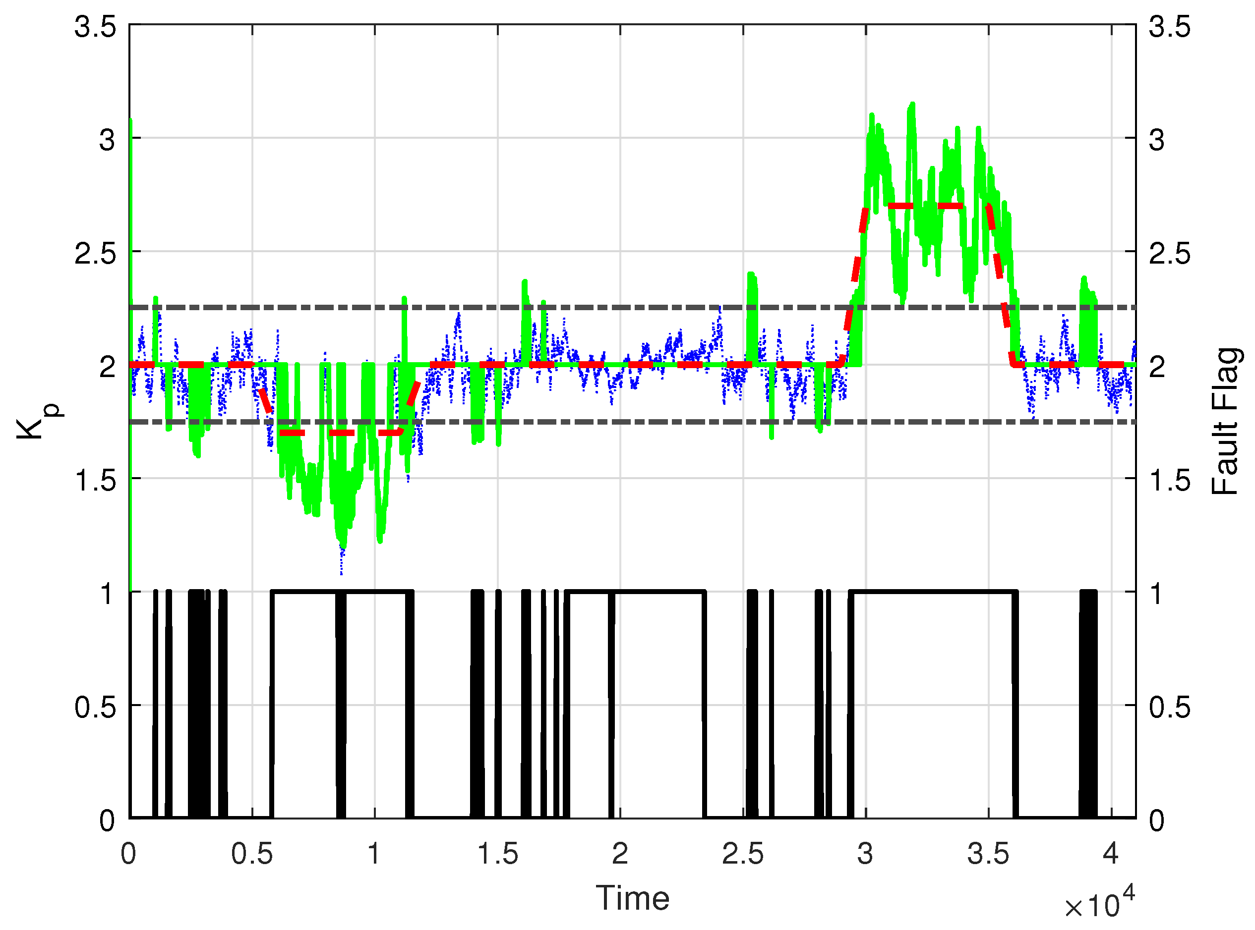
The next step is to couple the fault-detection mechanism of Theorem 2 with the fault-identification mechanism from Theorem 3. The result for , subject to the proposed faults, is shown in Figure 6. We observe that the inclusion of further discrimination by means of the estimated standard deviation , represented by the black dashed line, reduces the effect of false negative errors and false positive errors. Moreover, during the second fault, starting at 17,001, which is due only to a change in , the introduction of the -based discriminant in Theorem 3 allows the plant model gain to remain at the correct value, .
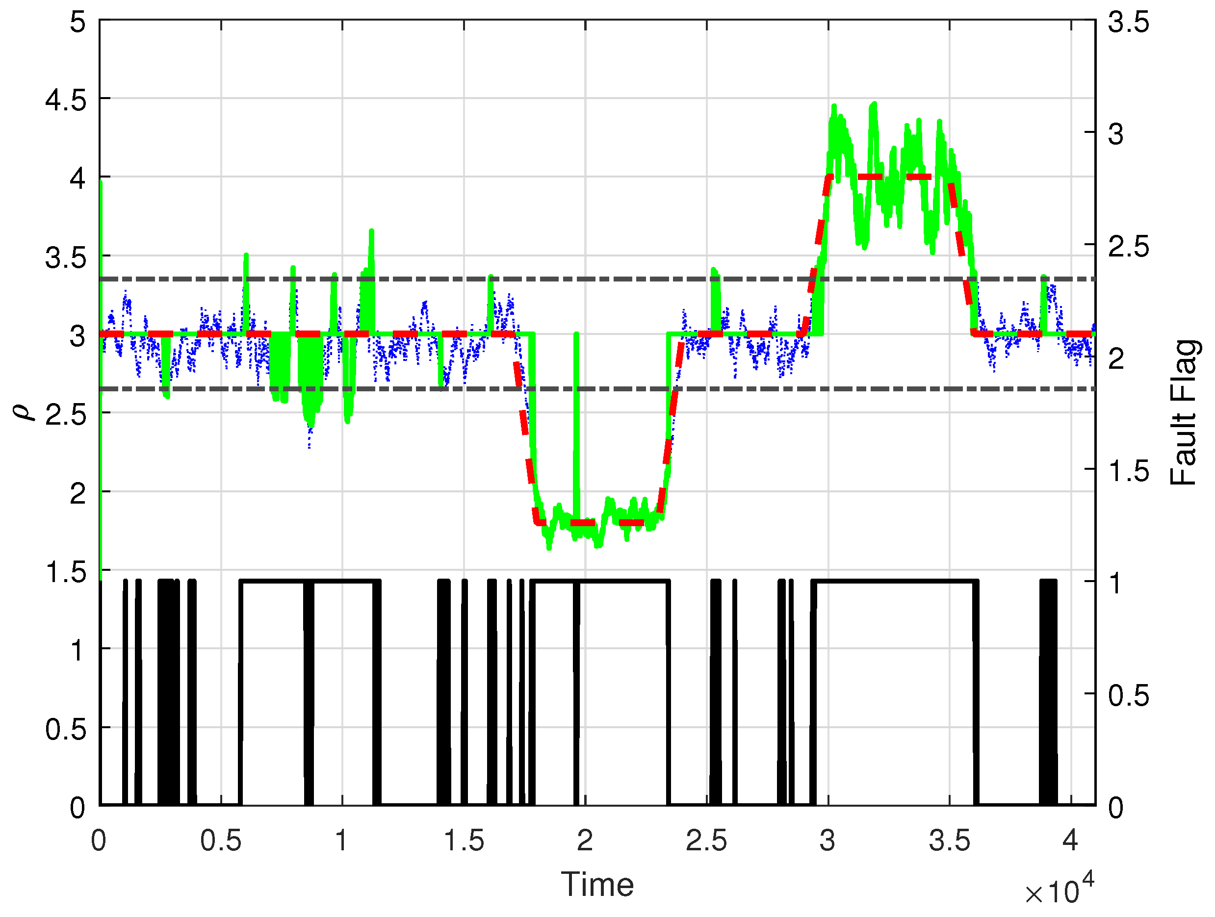
We conclude the example by reviewing the estimation of the unstable plant pole value, , subject to the faults in Figure 7 (green solid line). As we can see, the introduction of the standard deviation discriminant, , was not as successful as for the plant model gain in avoiding a noisy estimation during the first fault starting at , even though this first fault is only due to a change in the value of . Moreover, during the second fault, due only to a change in the value of the unstable plant pole, a false negative error is still present in the proposed identification at approximately 20,000. Nevertheless, some instances of false negative errors were suppressed between the first and second faults and at the end of the simulation run.
7. Conclusions
In this work, we propose an optimal NCS design subject to a network of simultaneous power-constrained AWGN channels over direct and feedback paths. The optimal controller design is then the foundation of a differential entropy estimation fault-detection mechanism. The use of differential entropy is justified by the presence of the AWGN channel and is also reasonable since it introduces a logarithmic scale on the channel over the direct-path input variance, which can otherwise result in very large excursions when subjected to faults, as observed in the provided example. The last contribution is a fault-identification mechanism restricted to the signals available on the controller side of the network, namely, u and . A limitation of the proposed fault-detection method is the trade-off imposed by the choice of L. The smaller the value of L is, the larger the value of is because of and , and vice versa. Since the value of determines the sensitivity of the fault-detection mechanism, an experienced user must strike the right compromise between these two design parameters. Additionally, as a future research direction, the imposed side restriction signal availability, due to the NCS nature of the closed control loop, can be explored to improve the use of signals on the plant side of the network in the design of a fault-detection/identification mechanism. Finally, once the faults are successfully identified, they should be used for retuning the optimal controller in an adaptive scheme that allows for fault recovery.
Funding
This research was funded by ANID Fondecyt Regular grant number 1230777 and ANID Basal Project AC3E grant number FB0008.
Data Availability Statement
Data is contained within the article.
Conflicts of Interest
The author declares no conflicts of interest.
References
- Levine, W.S.E. The Control Handbook; CRC Press: Boca Raton, FL, USA, 1996. [Google Scholar]
- Du, B.; Xu, Q.; Zhang, J.; Tang, Y.; Wang, L.; Yuan, R.; Yuan, Y.; An, J. Periodic Intermittent Adaptive Control with Saturation for Pinning Quasi-Consensus of Heterogeneous Multi-Agent Systems with External Disturbances. Entropy 2023, 25, 1266. [Google Scholar] [CrossRef]
- Cetinkaya, A.; Ishii, H.; Hayakawa, T. An Overview on Denial-of-Service Attacks in Control Systems: Attack Models and Security Analyses. Entropy 2019, 21, 210. [Google Scholar] [CrossRef]
- Qin, C.; Wu, Y.; Zhang, J.; Zhu, T. Reinforcement Learning-Based Decentralized Safety Control for Constrained Interconnected Nonlinear Safety-Critical Systems. Entropy 2023, 25, 1158. [Google Scholar] [CrossRef] [PubMed]
- Zhang, Y.; Jia, Y.; Chai, T.; Wang, D.; Dai, W.; Fu, J. Data-Driven PID Controller and Its Application to Pulp Neutralization Process. IEEE Trans. Control. Syst. Technol. 2018, 26, 828–841. [Google Scholar] [CrossRef]
- Nair, G.; Evans, R. Stabilizability of stochastic linear systems with finite feedback data rates. SIAM J. Control Optim. 2004, 43, 413–436. [Google Scholar] [CrossRef]
- Martins, N.; Dahleh, M. Feedback Control in the Presence of Noisy Channels: “Bode-Like” Fundamental Limitations of Performance. IEEE Trans. Autom. Control 2008, 53, 1604–1615. [Google Scholar] [CrossRef]
- Elia, N. When Bode Meets Shannon: Control Oriented Feedback Communication Schemes. IEEE Trans. Autom. Control 2004, 49, 1477–1488. [Google Scholar] [CrossRef]
- Braslavsky, J.; Middleton, R.; Freudenberg, J. Feedback Stabilisation over Signal-to-Noise Ratio Constrained Channels. IEEE Trans. Autom. Control 2007, 52, 1391–1403. [Google Scholar] [CrossRef]
- Rojas, A. Signal-to-noise ratio fundamental limitations in the discrete-time domain. Syst. Control Lett. 2012, 61, 55–61. [Google Scholar] [CrossRef]
- da Silva, J., Jr.; Lages, W.; Sbarbaro, D. Event-triggered PI control design. In Proceedings of the 19th IFAC World Congress, Cape Town, South Africa, 24–29 August 2014; pp. 6947–6952. [Google Scholar]
- Campos-Delgado, D.U.; Rojas, A.J.; Luna-Rivera, J.M.; Gutiérrez, C.A. Event-triggered feedback for power allocation in wireless networks. IET Control Theory Appl. 2015, 9, 2066–2074. [Google Scholar] [CrossRef]
- Ma, Y.; Gu, C.; Liu, Y.; Yu, L.; Tang, W. Event-Triggered Bounded Consensus Tracking for Second-Order Nonlinear Multi-Agent Systems with Uncertainties. Entropy 2023, 25, 1335. [Google Scholar] [CrossRef]
- Zhao, J.; Wang, Y.; Gao, P.; Li, S.; Peng, Y. Synchronization of Complex Dynamical Networks with Stochastic Links Dynamics. Entropy 2023, 25, 1457. [Google Scholar] [CrossRef] [PubMed]
- Gertler, J. Fault Detection and Diagnosis in Engineering Systems; Marcel Dekker: New York, NY, USA, 1998. [Google Scholar]
- Chen, J.; Patton, R.J. Robust Model-Based Fault Diagnosis for Dynamic Systems; Kluwer Academic Publishers: London, UK, 1999. [Google Scholar]
- Blanke, M.; Kinnaert, M.; Lunze, J.; Staroswiecki, M. Diagnosis and Fault-Tolerant Control; Springer: Berlin, Germany, 2003. [Google Scholar]
- Saberi, A.; Stoorvogel, A.A.; Sannuti, P. Filtering Theory: With Applications to Fault Detection, Isolation, and Estimation; Birkhauser: Basel, Switzerland, 2007. [Google Scholar]
- Varga, A. Solving Fault Diagnosis Problems: Linear Synthesis Techniques; Studies in Systems, Decision and Control; Springer: Berlin/Heidelberg, Germany, 2017. [Google Scholar]
- Ding, S.X.; Frank, P.M.; Ding, E.L.; Jeinsch, T. A unified approach to the optimizaton of fault detection systems. Int. J. Adapt. Control Signal Process. 2000, 14, 725–745. [Google Scholar] [CrossRef]
- Saberi, A.; Stoorvogel, A.A.; Sannuti, P.; Niemann, H. Fundamental problems in fault detection and identification. Int. J. Robust Nonlinear Control 2000, 10, 1209–1236. [Google Scholar] [CrossRef]
- Gao, Z.; Cecati, C.; Ding, S.X. A Survey of Fault Diagnosis and Fault-Tolerant Techniques—Part I: Fault Diagnosis with Model-Based and Signal-Based Approaches. IEEE Trans. Ind. Electron. 2015, 62, 3757–3767. [Google Scholar] [CrossRef]
- Gao, Z.; Cecati, C.; Ding, S.X. A Survey of Fault Diagnosis and Fault-Tolerant Techniques—Part II: Fault Diagnosis with Knowledge-Based and Hybrid/Active Approaches. IEEE Trans. Ind. Electron. 2015, 62, 3768–3774. [Google Scholar] [CrossRef]
- Ding, S. A survey of fault-tolerant networked control system design. In Proceedings of the 8th IFAC Symposium on Fault Detection, Supervision and Safety of Technical Processes, Mexico City, Mexico, 29–31 August 2012; pp. 874–885. [Google Scholar]
- Aubrun, C.; Sauter, D.; Yame, J. Fault diagnosis of networked control systems. Int. J. Appl. Math. Comput. Sci. 2008, 18, 525–537. [Google Scholar] [CrossRef]
- Ren, W.; Sun, S.; Hou, N.; Kang, C. Event-triggered non-fragile h infinity fault detection for discrete time-delayed nonlinear systems with channel fadings. J. Frankl. Inst. 2018, 355, 436–457. [Google Scholar] [CrossRef]
- Lami, Y.; Lefevre, L.; Lagreze, A.; Genon-Catalot, D. A Bayesian Approach for Fault Diagnosis in an Irrigation Canal. In Proceedings of the 24th International Conference on System Theory, Control and Computing, Sinaia, Romania, 8–10 October 2020; pp. 328–335. [Google Scholar]
- Li, W.; Zhu, Z.; Ding, X. On Fault Detection Design of Networked Control Systems. In Proceedings of the 8th IFAC Symposium on Fault Detection, Supervision and Safety of Technical Processes, Barcelona, Spain, 30 June–3 July 2009; pp. 792–797. [Google Scholar]
- Bahreini, M.; Zarei, J. Robust fault-tolerant control for networked control systems subject to random delays via static-output feedback. ISA Trans. 2019, 86, 153–162. [Google Scholar] [CrossRef]
- Schenk, K.; Lunze, J. Fault-Tolerant Task Allocation in Networked Control Systems. In Proceedings of the 28th Mediterranean Conference on Control and Automation, Saint-Raphael, France, 15–18 September 2020; pp. 313–318. [Google Scholar]
- Wang, B.; Zhang, B.; Su, R. Optimal Tracking Cooperative Control for Cyber-Physical Systems: Dynamic Fault-Tolerant Control and Resilient Management. IEEE Trans. Ind. Inform. 2021, 17, 158–167. [Google Scholar] [CrossRef]
- Wang, T.; Gao, H.; Qiu, J. A Combined Fault-Tolerant and Predictive Control for Network-Based Industrial Processes. IEEE Trans. Ind. Electron. 2016, 63, 2529–2536. [Google Scholar] [CrossRef]
- Rojas, A.; Braslavsky, J.; Middleton, R. Fundamental limitations in control over a communication channel. Automatica 2008, 12, 3147–3151. [Google Scholar] [CrossRef]
- Åström, K. Introduction to Stochastic Control Theory; Academic Press: Cambridge, MA, USA, 1970. [Google Scholar]
- Bertesekas, D.P. Convex Optimzation Theory; Athena Scientific: Nashua, NH, USA, 2009. [Google Scholar]
- Cover, T.; Thomas, J. Elements of Information Theory; John Wiley & Sons: Hoboken, NJ, USA, 1991. [Google Scholar]
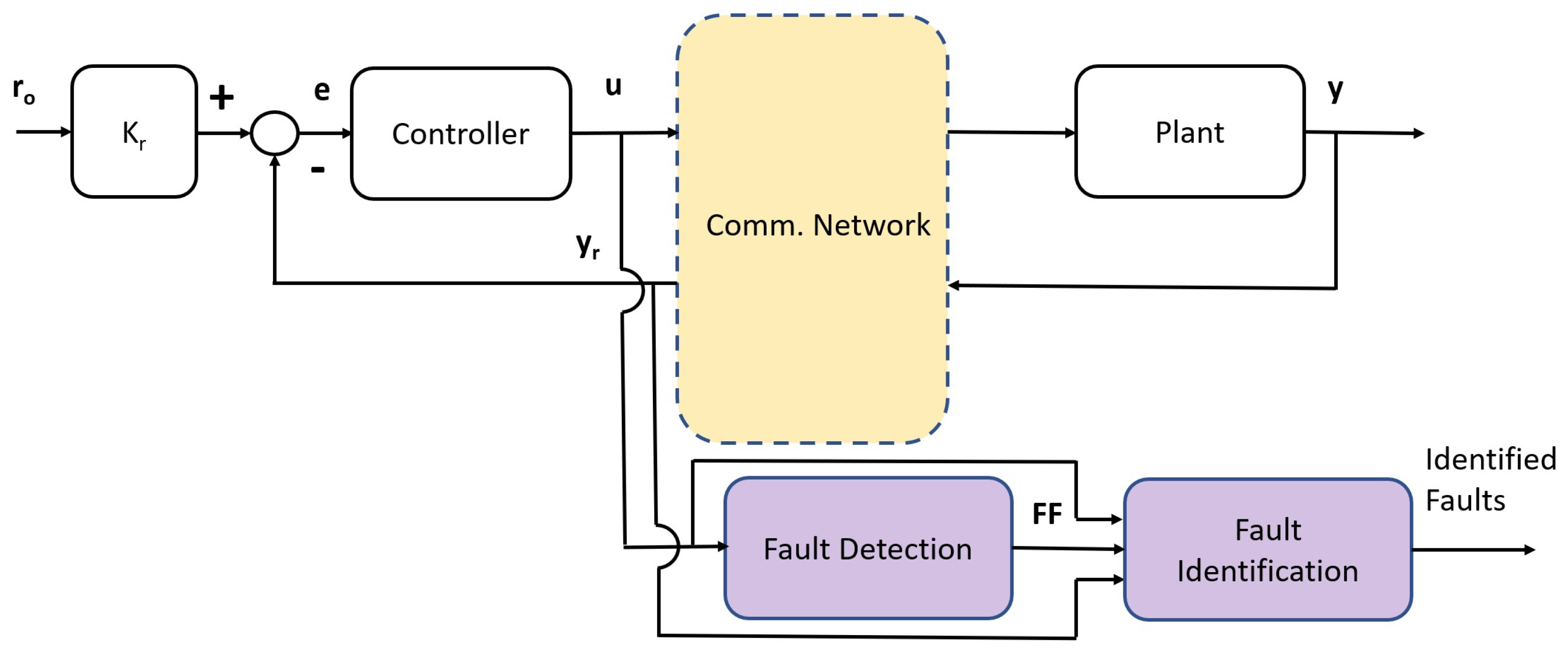
Figure 1.
NCS SISO feedback loop with residual generator and fault-detection stages.

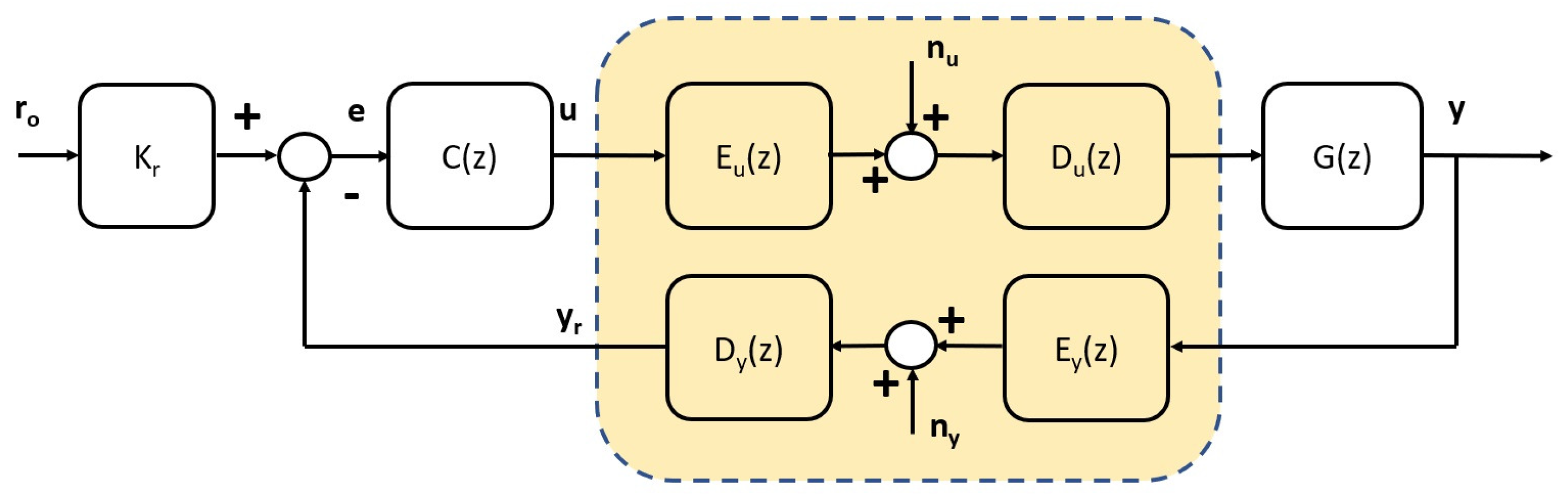
Figure 2.
NCS SISO feedback loop with an AWGN network.

Figure 3.
Monte Carlo simulation of as a function of L for (blue dots), predicted mean value (red dashed line), and variance of as a function of L (black dash-dotted line).
Figure 3.
Monte Carlo simulation of as a function of L for (blue dots), predicted mean value (red dashed line), and variance of as a function of L (black dash-dotted line).

Figure 4.
Estimated differential entropy of the signal , when no faults are present, for the selected value of (green solid line), no-fault theoretical value (red dashed line), and no-fault theoretical value plus two standard deviations (black dash-dotted lines).
Figure 4.
Estimated differential entropy of the signal , when no faults are present, for the selected value of (green solid line), no-fault theoretical value (red dashed line), and no-fault theoretical value plus two standard deviations (black dash-dotted lines).

Figure 5.
Estimated differential entropy of the signal , when faults in (21) and (22) are present, for the selected value of (green solid line), no-fault theoretical value (red dashed line), and no-fault theoretical value plus two standard deviations (black dash-dotted lines).

Figure 6.
Estimated value of the plant gain parameter for the selected value of (green solid line), true parameter value (red dashed line), standard deviation (black dash-dotted line), and reported fault flag (black solid line at the bottom).
Figure 6.
Estimated value of the plant gain parameter for the selected value of (green solid line), true parameter value (red dashed line), standard deviation (black dash-dotted line), and reported fault flag (black solid line at the bottom).

Figure 7.
Estimated value of the plant gain parameter, , for the selected value of (green solid line), true parameter value (red dashed line), standard deviation (black dash-dotted line), and reported fault flag (black solid line at the bottom).
Figure 7.
Estimated value of the plant gain parameter, , for the selected value of (green solid line), true parameter value (red dashed line), standard deviation (black dash-dotted line), and reported fault flag (black solid line at the bottom).

Disclaimer/Publisher’s Note: The statements, opinions and data contained in all publications are solely those of the individual author(s) and contributor(s) and not of MDPI and/or the editor(s). MDPI and/or the editor(s) disclaim responsibility for any injury to people or property resulting from any ideas, methods, instructions or products referred to in the content. |
© 2024 by the author. Licensee MDPI, Basel, Switzerland. This article is an open access article distributed under the terms and conditions of the Creative Commons Attribution (CC BY) license (https://creativecommons.org/licenses/by/4.0/).
Share and Cite
MDPI and ACS Style
Rojas, A.J. Differential Entropy-Based Fault-Detection Mechanism for Power-Constrained Networked Control Systems. Entropy 2024, 26, 259. https://doi.org/10.3390/e26030259
AMA Style
Rojas AJ. Differential Entropy-Based Fault-Detection Mechanism for Power-Constrained Networked Control Systems. Entropy. 2024; 26(3):259. https://doi.org/10.3390/e26030259
Chicago/Turabian StyleRojas, Alejandro J. 2024. "Differential Entropy-Based Fault-Detection Mechanism for Power-Constrained Networked Control Systems" Entropy 26, no. 3: 259. https://doi.org/10.3390/e26030259
Note that from the first issue of 2016, this journal uses article numbers instead of page numbers. See further details here.