

The Kaniadakis Distribution for the Analysis of Income and Wealth Data


Department of Political Science, Communication and International Relations, University of Macerata, Via Don Minzoni 22/A, 62100 Macerata, Italy
Entropy 2023, 25(8), 1141; https://doi.org/10.3390/e25081141
Submission received: 27 June 2023
/
Revised: 27 July 2023
/
Accepted: 28 July 2023
/
Published: 30 July 2023
(This article belongs to the Special Issue Twenty Years of Kaniadakis Entropy: Current Trends and Future Perspectives)
Abstract
:The paper reviews the “-generalized distribution”, a statistical model for the analysis of income data. Basic analytical properties, interrelationships with other distributions, and standard measures of inequality such as the Gini index and the Lorenz curve are covered. An extension of the basic model that best fits wealth data is also discussed. The new and old empirical evidence presented in the article shows that the -generalized model of income/wealth is often in very good agreement with the observed data.
1. Introduction
The past two decades have seen a resurgence of interest in the study of income and wealth distribution in both the physics [1,2,3,4] and economics [5,6,7,8,9] communities. Scholars have focused particularly on the empirical analysis of large data sets to infer the shape of income and wealth distributions and to develop theoretical models that can reproduce them.
Pareto’s observation that the number of people in a population whose income exceeds x is often well approximated by was a natural starting point for this field of analysis [10,11,12,13]. However, empirical research has shown that the Pareto distribution accurately models only high income levels, while it does a poor job of describing the lower end of distributions.
As research has continued, new models have been proposed to better describe the data, using either a combination of known statistical distributions [14,15,16,17,18,19,20,21,22] or parametric functional forms for the distribution as a whole. Among these, the two-parameter lognormal [23] and gamma [24] distributions were proposed as models for the size distributions of income and wealth, but later evidence showed that these models tend to exaggerate skewness and perform poorly at the upper end of the empirical distributions [25,26,27,28]. Three-parameter models such as the generalized gamma [29,30,31,32], Singh–Maddala [33], and Dagum Type I [34] provide better fits. These models converge to the Pareto model for large values of income/wealth and accurately describe lower and middle ranges.
Finally, models with more than three parameters have also been suggested to fit income and wealth data. For example, the generalized beta distribution of the second kind (GB2) is a four-parameter distribution that was first described by [35]. It fits the data very well and also includes some of the two- and three-parameter models mentioned above as special or limiting cases. (The generalized beta distribution of the first kind (GB1) [35] and the double Pareto-lognormal distribution [36] are other four-parameter models that fit the data well. Ref. [37] also developed the five-parameter generalized beta distribution family, which includes the GB1 and GB2 as special cases and all of the two- and three-parameter distributions nested inside them. In turn, the double Pareto-lognormal distribution has been generalized into a five-parameter family of distributions called the generalized double Pareto-lognormal distribution [38]. However, closed-form expressions for probability density and/or cumulative distribution functions do not always exist for these “super” models, making fitting them to data computationally difficult and slow due to the need to use numerical methods [39,40]).
Among models that seek to provide a unified framework for describing real-world data, including the power-law tails found in empirical distributions of income and wealth, the -generalized distribution has demonstrated exceptional performance and is often seen as a better alternative to other widely used parametric models. This model, which was initially introduced in 2007 and progressively expanded in the years that followed, has its origins in the framework of -generalized statistical mechanics [41,42,43,44,45,46]. It has a bulk very similar to the Weibull distribution and an upper tail that decays according to a Pareto power law for high values of income and wealth, providing a sort of middle ground between the two descriptions.
The purpose of this paper is to provide a comprehensive overview of the important results concerning the -generalized distribution. The desire to celebrate the 20th anniversary of Kaniadakis’ notable contribution and the belief that an interdisciplinary approach integrating statistical mechanics and economics may give novel insights into economic relationships motivated this work. Giorgio Kaniadakis played a pivotal role in the development of the -generalized model, making valuable and direct contributions to its conception. The intention behind presenting information on the fundamental statistical properties and empirical plausibility of this distribution is to convince the reader of its importance and usefulness for future exploration.
The paper is structured as follows. Section 2 introduces the -generalized model, covering topics such as interrelations with other distributions, basic statistical properties, and inferential aspects. Section 3 presents recent results of fitting the -generalized distribution to empirical income data corresponding to the distribution of household incomes in Greece, and compares the relative merits of alternative income size distribution models using the same data. Section 4 reviews empirical applications showing that the -generalized model is often in excellent agreement with observed income data; the -generalized mixture model for net worth distribution, which best fits wealth data, is also discussed in this section. Section 5 concludes the paper with some remarks.
2. The -Generalized Model for Income Distribution
The -generalized statistical model, named after [47], is based on the use of -deformed exponential and logarithmic functions introduced by Kaniadakis [41,42,43] in the context of special relativity. Within this framework, the ordinary exponential function deforms into the generalized exponential function given by:
The deformed logarithmic function , which is defined as the inverse of (1), can be written as:
Kaniadakis’ deformed functions have also been successfully used to analyze nonphysical systems. In economics, the -deformation has been used to study differentiated product markets [48,49], finance [50,51,52,53,54,55], and the distribution of income by size [47,56,57,58,59,60,61,62]. In the latter case, it is interesting to use such deformed functions because they can be used to statistically describe the entire spectrum of incomes, from the low to the middle range and up to the Pareto tail.
2.1. Definitions and Basic Properties
A random variable X is said to have a -generalized distribution, and we write , if it has a probability density function (PDF) given by:
Its cumulative distribution function (CDF) can be expressed as:
(For a complete description of the -generalized distributional properties, the reader is referred to [60] and the references cited therein. A heuristic derivation of the -generalized density, showing how this probability distribution emerges naturally within the field of -deformed analysis, is given in [61,63]).
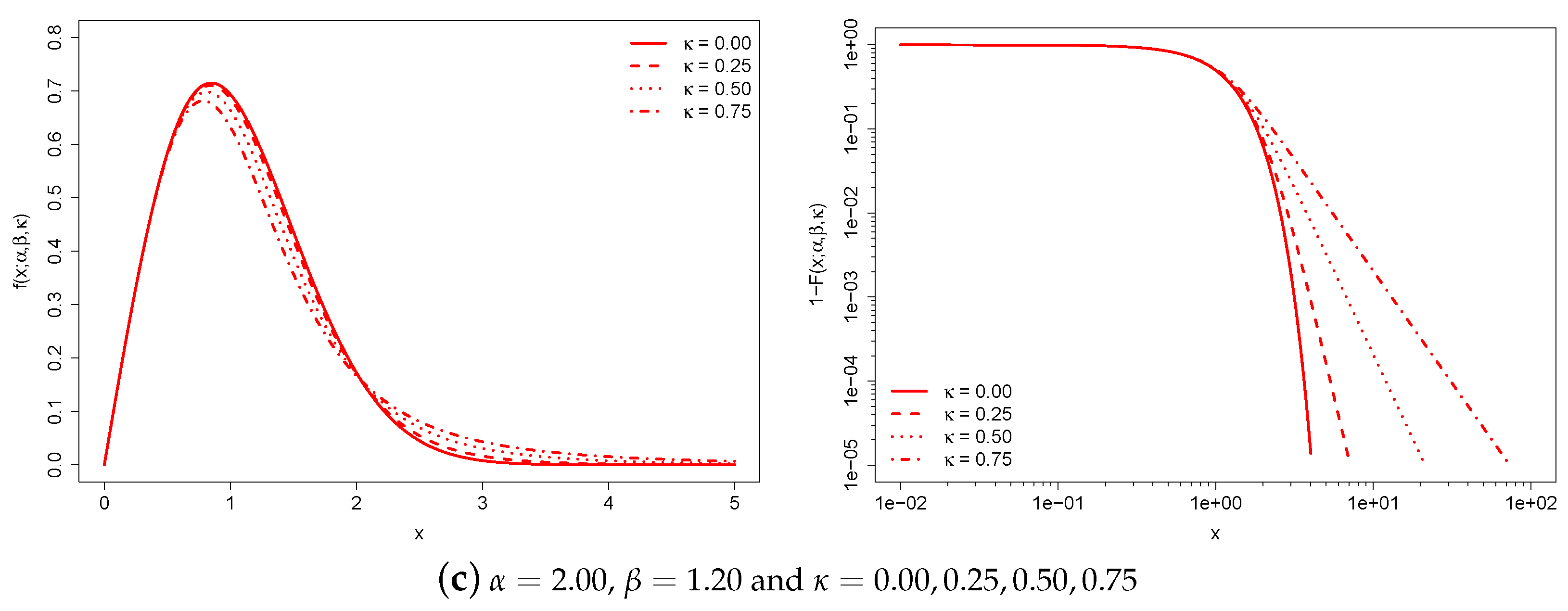
Figure 1 illustrates the behavior of the -generalized PDF and the complementary CDF, , for various parameter values.
Each of the three graph pairs holds two parameters constant and varies the remaining one.
The constant is a characteristic scale that has the same dimension as income. For this reason, it takes into account the monetary unit and can be used to adjust for inflation and facilitate cross-country comparisons of income distributions expressed in different monetary units. Increases in the monetary unit result in a global increase in individual income and average income.
The and parameters are scale-free parameters that affect the distribution’s shape. The region around the origin of the -generalized distribution is dominated by , while the upper tail is dominated by both and . Increasing leads to a thicker upper tail, while increasing tapers both tails and increases the concentration of probability mass around the peak of the distribution.
As approaches 0, the distribution converges to the Weibull distribution; it is easy to verify that:
and:
(The Weibull distribution is primarily studied in the engineering literature. In physics, it is known as the stretched exponential distribution when . In economics, it has potential for income data, although it has only been used sporadically—some applications can be found in Refs. [29,35,64,65,66,67,68,69].) The distribution behaves similarly to the Weibull model for , while for large x it approaches a Pareto distribution of the first kind with scale and shape , i.e.:
and:
thus satisfying the weak Pareto law [70]. (Additional versions of the Pareto law were introduced by [71], , and [30], . Since we have: and , the -generalized distribution also obeys these alternative versions of the weak Pareto law.)
Equation (4) implies that the quantile function is available in closed form:
an attractive feature for generating random numbers from a -generalized distribution. The median of the distribution is:
and the mode occurs at:
if ; otherwise, the distribution is zero-modal with a pole at the origin.
Finally, the rth raw moment of the -generalized distribution is equal to:
where denotes the gamma function, and exists for . Specifically:
is the mean of the distribution and:
is the variance.
2.2. Measuring Income Inequality Using the -Generalized Distribution
The concept of inequality in economics dates back to Pareto’s early work [10,11,12,13], which showed that the top 20% of population held about 80% of total income/wealth. Later, the American economist Lorenz [72] introduced the Lorenz curve, a widely used tool for measuring income/wealth inequality. This curve measures the difference in income or wealth distribution from an equal distribution. If there is perfect equality, the Lorenz curve coincides with the diagonal of a unit square, while worsening distribution (more inequality) moves the curve away from the diagonal.
The Lorenz curve for a random variable X with CDF and finite mean is defined as [73]:
Using the closed form of the quantile function of the -generalized distribution, the Lorenz curve can be reformulated as follows [74]:
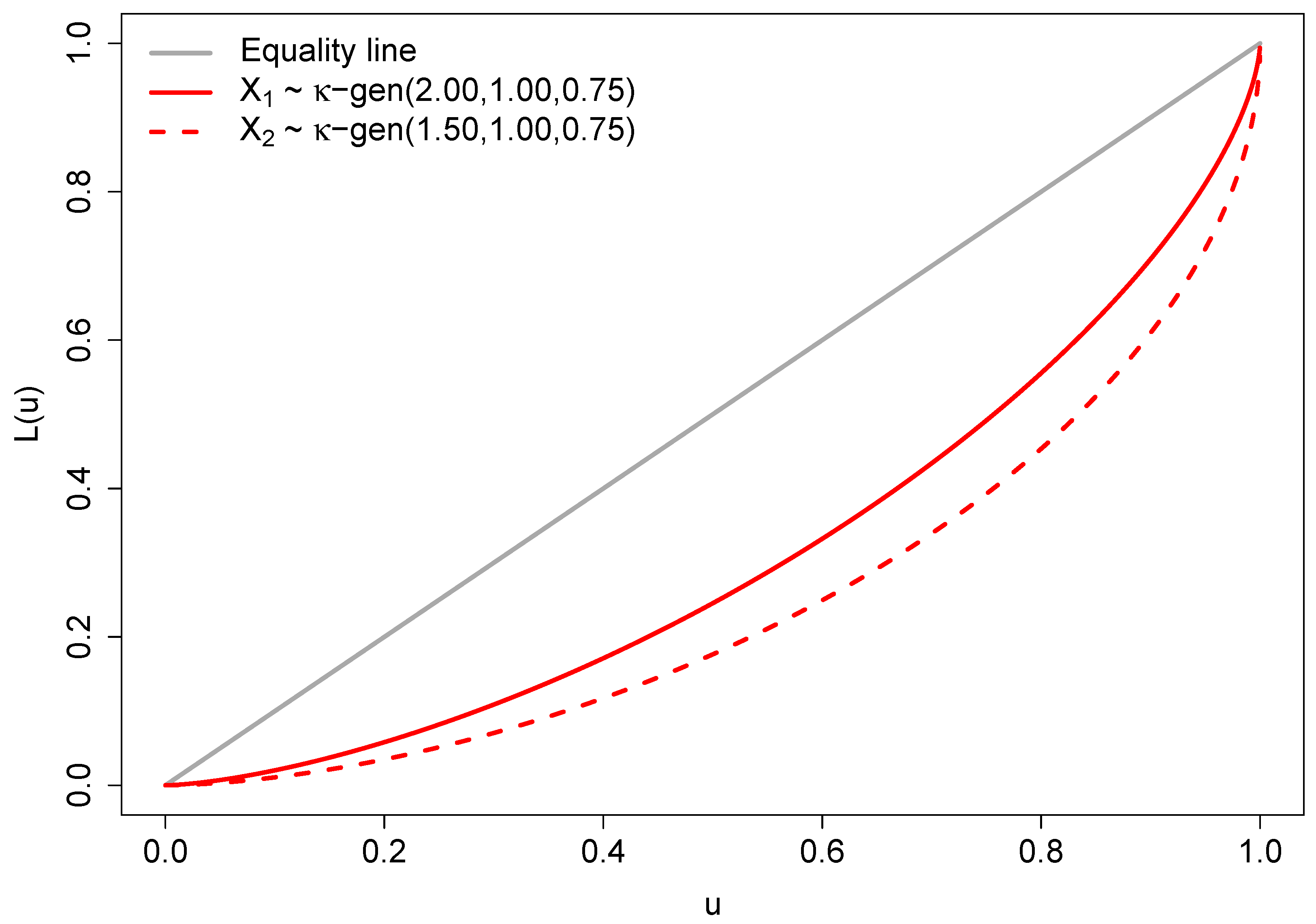
where is the regularized incomplete beta function defined in terms of the incomplete beta function and the complete beta function, that is, . The curve (16) exists if and only if . In particular, if , , the necessary and sufficient conditions for the Lorenz curves of and not to intersect (otherwise, it would be impossible to determine which distribution has more inequality) are [58]:
The Lorenz curves of two -generalized distributions and with parameters chosen according to (17) are illustrated in Figure 2. The depicted curves indicate that exhibits lower inequality compared to , as the Lorenz curve of does not intersect or fall below that of .
Economists have employed statistical metrics to quantify income and wealth inequality. The Gini coefficient, developed in 1914 by the Italian statistician Gini [75], is one of the best known. From the general definition due to [76], the Gini coefficient associated with the -generalized distribution is:
Using the Stirling approximation for the gamma function, , and taking the limit as in Equation (18), after some simplification one arrives at , which is the explicit form of the Gini coefficient for the Weibull distribution (see e.g., [77], p. 177). Since the exponential distribution is a special case of the Weibull distribution with a shape parameter of 1, it follows directly that for and , the exponential law is also a special limiting case of the -generalized distribution with a true Gini coefficient of one half [16].
The Gini coefficient is a widely used measure of inequality, but it makes specific assumptions about income differences in different parts of the distribution. It is most sensitive to transfers around the middle of the income distribution and least sensitive to transfers among the very rich or very poor [78]. Differently, the generalized entropy class of inequality measures [79,80,81,82,83] provides a range of bottom-to-top sensitive indices used by analysts to assess inequality in different parts of the income distribution. The expression for this class of inequality indices in terms of the -generalized parameters is [57]:
where denotes the mean of the distribution given by Equation (13). Formula (19) defines a class because takes different forms depending on the value given to , the parameter that describes the sensitivity of the index to income differences in different parts of the income distribution—the more positive or negative is, the more sensitive is to income differences at the top or bottom of the distribution. Two limiting cases of (19), obtained when the parameter is set to 0 and 1, have gained attention in practical work for the purpose of measuring inequality; these are the mean logarithmic deviation index:
where is the Euler–Mascheroni constant and is the digamma function, and the Theil index [84]:
where the former is more sensitive to variations in the lower tail, while the latter is more sensitive to variations in the upper tail [85]. (Equation (19) is not defined for and , as in both cases. Expressions for these values of are therefore derived using l’Hôpital rule, which allows evaluating limits of indeterminate forms using derivatives. Expressions for any index other than the cases can be derived by simple substitution—see for example [60]).
Finally, the class of inequality measures introduced by Atkinson [86] can be derived from (19) by exploiting the relationship [87,88]:
where is the inequality aversion parameter. As increases, becomes more sensitive to transfers among lower incomes and less sensitive to transfers among top incomes [78]. The limiting form of (22) is . (All measures considered here are functions of distributional moments, whose existence depends on conditions assuring the convergence of the appropriate integrals. The Gini coefficient (18) exists if and only if the mean of the distribution converges, which is true if and only if . According to [89], parametric income distribution models share the existence problem of popular inequality measures).
2.3. Estimation
The -generalized distribution’s parameters can be estimated using the maximum likelihood technique, which produces estimators with good statistical properties [90,91]. If sample observations are independent, the likelihood function is as follows:
where denotes the PDF, the vector of unknown parameters, the weight of the ith observation, and n the sample size. This leads to the problem of solving the partial derivatives with respect to , and for the log-likelihood function:
which is the same as finding the solution to the following nonlinear system of equations:
However, the derivation of explicit expressions for maximum likelihood estimators of the three -generalized parameters poses a challenge due to the absence of feasible analytical solutions. The utilization of numerical optimization algorithms becomes therefore imperative in order to solve the maximum likelihood estimation problem.
3. Application to the Income Distribution in Greece
To celebrate 20 years of Kaniadakis’ contribution, it seems appropriate to consider the income distribution in his native Greece to demonstrate the -generalized model’s capacity to fit real-world data. First, income data for parameter estimation are briefly described. Next, the -generalized distribution is fitted to Greek household income data. Finally, using the same income microdata, different income size distribution models are compared.
3.1. Description of the Income Data
Income distribution data for Greece were obtained from the Luxembourg Income Study (LIS) database, which provides public access to household-level data files for various countries, including both developed and developing economies. The data are remote-accessible, requiring program code to be sent to LIS rather than being run directly by the user. At the time of writing, LIS contains Greek income distribution data for the following years: 1995, 2000, 2004, 2007, 2010, 2013, and 2016. The data set used for this review is the 2016 data set based on the 2017 wave of the Greek EU-SILC survey conducted by the Hellenic Statistical Authority (ELSTAT). (EU-SILC is a cross-sectional and longitudinal sample survey coordinated by Eurostat, focusing on income, poverty, social exclusion, and living conditions in the European Union.) The sample size is 22,555 households.
The definition of income is “household disposable income”, which is the income available to households to support consumption expenditure and saving during the reference period. The measure includes income from work, wealth, and direct government benefits, but subtracts direct taxes paid. It does not include sales taxes or noncash benefits, such as healthcare provided by a government or employer. Additionally, the income definition excludes income from capital gains, a significant source of nonwage income for wealthy individuals. As a result, many top incomes are likely to be underestimated.
Household disposable income is expressed in euro and “equivalized”, i.e., divided by the square root of household size to adjust for differences in household demographics. Prior to equivalization, top and bottom coding is applied to set limits for extreme values. We also exclude all households with missing disposable income and use person-adjusted weights (the product of the household weights and the number of household members) when generating income indicators for the total population and estimating model parameters.
3.2. Results of Fitting
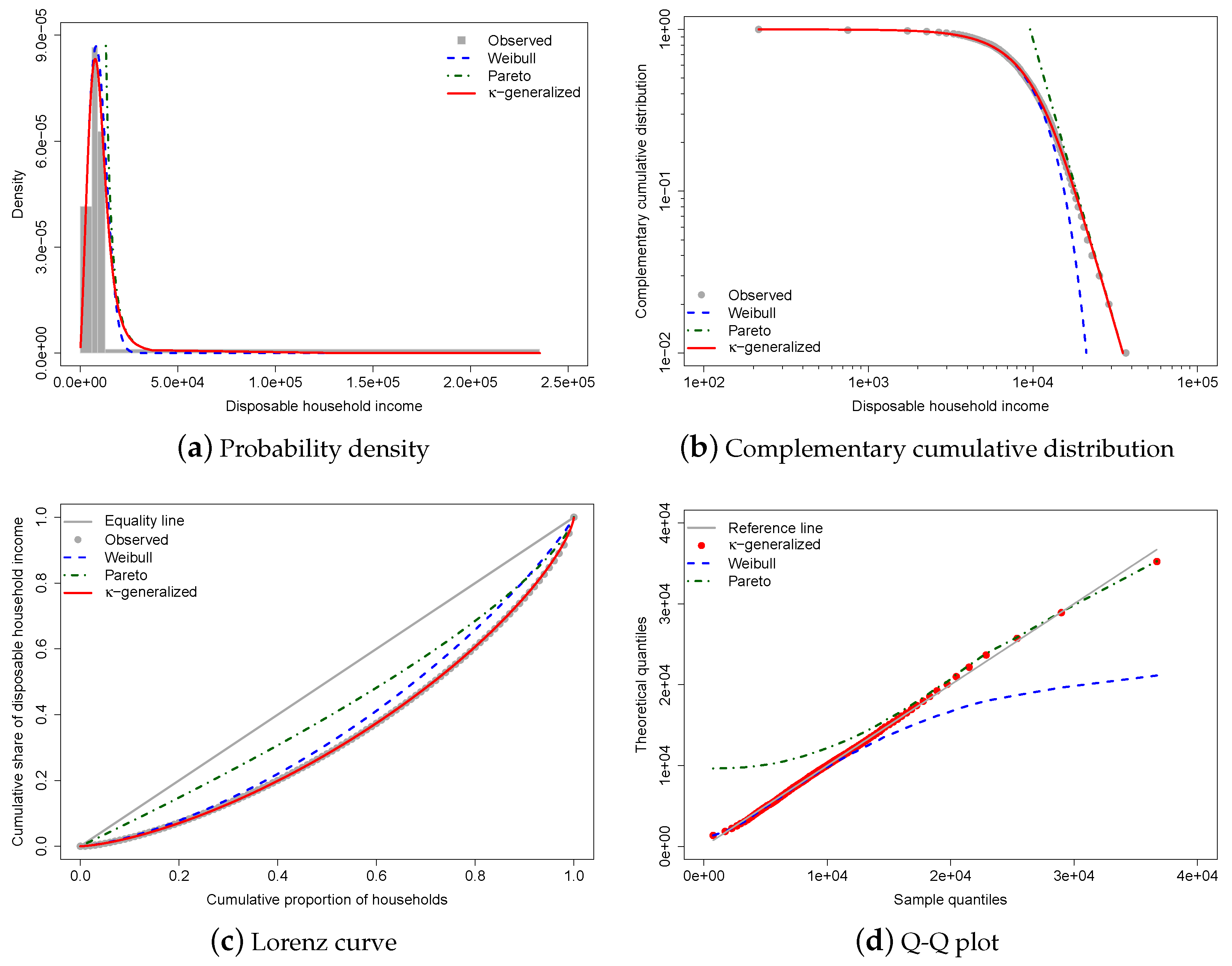
Figure 3 shows the results of fitting the -generalized distribution to empirical income data corresponding to the distribution of household income in Greece for the year 2016.
The best-fitting parameter values were determined using maximum likelihood estimation, resulting in estimates of , , and . The small errors indicate accurate estimations, and the comparison between the observed and fitted probabilities in panels (a) and (b) of Figure 3 suggests that the -generalized distribution has great potential for describing data across the range of low-to-middle-income to high-income power-law regimes, including the intermediate region where Weibull and Pareto distributions show clear departures. (In Figure 3, the curves for the Pareto and Weibull distributions have been drawn by expressing their parameters in terms of the estimated -generalized parameters—see Section 2.1).
Panel (c) of the same figure displays data points for the empirical Lorenz curve superimposed on the theoretical curve given by Equation (16) with estimates replacing and as necessary. This formula, represented by the red solid line in the plot, matches the data exceptionally well. In addition, the plot contrasts the empirical Lorenz curve with the theoretical curves associated with the Weibull and Pareto distributions, respectively, given by:
where is the lower regularized incomplete gamma function, and:
As one can easily see, these curves tell only a small part of the story.
To provide an indirect check on the validity of the parameter estimation, we have also computed predicted values for median and mean household disposable income, as well as the Gini and Atkinson coefficients—the latter with the inequality aversion parameter equal to 1. The results, obtained by substituting the estimated parameters into relevant expressions, are presented in Table 1, along with their empirical counterparts, corresponding to the LIS staff’s “Inequality and Poverty Key Figures” for the considered country and year. (In this article, inequality measures are calculated using the most recent version of DASP, the Distributive Analysis Stata Package [92], which is available at http://dasp.ecn.ulaval.ca/—accessed on 26 June 2023. The complete set of corresponding “key figures” is available in an Excel workbook that can be downloaded from https://www.lisdatacenter.org/data-access/key-figures/—accessed on 26 June 2023).
The -generalized distribution predictions are fully covered by asymptotic normal 95% confidence intervals, confirming excellent agreement between the model and sample observations.
The linear behavior of the quantile-quantile (Q-Q) plot of sample percentiles against the fitted -generalized distribution and its limiting cases, shown in panel (d) of Figure 3, confirms the model’s validity as well as the fact that the Weibull and Pareto distributions provide partial and incomplete data descriptions.
3.3. Comparisons of Alternative Distributions
This section compares the -generalized distribution’s performance with other parametric models, including the three-parameter generalized gamma [93], Singh–Maddala [33], and Dagum type I [34] distributions, which have the following PDFs, respectively:
Ref. [77] provides analytical expressions for distribution functions, moments, and tools for inequality measurement, including the Lorenz curve and Gini coefficient. Refs. [87,94] provide formulas for generalized entropy measures of the GB2 distribution, from which the Singh–Maddala and Dagum versions are easily obtained. For the generalized gamma distribution, closed expressions for the Theil entropy index and the mean logarithmic deviation are given in Refs. [85,95]. (Let X be a random variable following the generalized beta distribution of the second kind (GB2) with parameters a, b, p, and q, i.e., . The Singh–Maddala distribution is the special case of the GB2 distribution when ; the Dagum type I distribution is the special case when . For a discussion of other special cases, see [35,77]).
Table 2 displays maximum likelihood estimates for the models under consideration.
The -generalized model offers the best results, with parameter standard errors derived from the inverse Hessian matrix being the lowest among competing income distribution models.
The root mean square error and mean absolute error between observed and predicted probabilities were used to determine which distribution best fits the data. These goodness-of-fit measures are, respectively, defined by:
and:
where , with , denotes the weighted empirical cumulative distribution function—equal to the sum of the income weights where divided by the total sum of weights—and is the vector of estimated parameters. (In the formulas above, is an indicator function that takes the value 1 if the condition in is true, 0 otherwise.) The and between the observed and estimated Lorenz curves have also been used as goodness-of-fit criteria, as they are expected to better reflect the accuracy of the inequality estimates. These additional measures are given by:
and:
where and denote the cumulative share of population and income, respectively, up to percentile i—i.e., is a point on the empirical Lorenz curve.
Based on the above goodness-of-fit criteria, the -generalized model is clearly the best fit. As shown in the last three columns of Table 2, the generalized gamma, Singh–Maddala, and Dagum type I have larger and values for both probabilities and Lorenz curves, suggesting that these models perform worse than the -generalized distribution.
The performance of the four models is further evaluated by considering the accuracy of selected distributional statistics implied by parameter estimates. Table 3 presents the predicted values for the median, mean, and several inequality measures derived from estimates in Table 2. (The Gini coefficient of the generalized gamma distribution is available in [35] as a long expression involving the Gaussian hypergeometric function , which is not currently available in the online statistical evaluator provided by the LIS web-based interface. An estimate of the Gini index for the generalized gamma distribution was therefore obtained by numerically integrating the area between the predicted Lorenz curve and the line of hypothetical equality. Ref. [96] reviews various methods for numerically estimating the Gini).
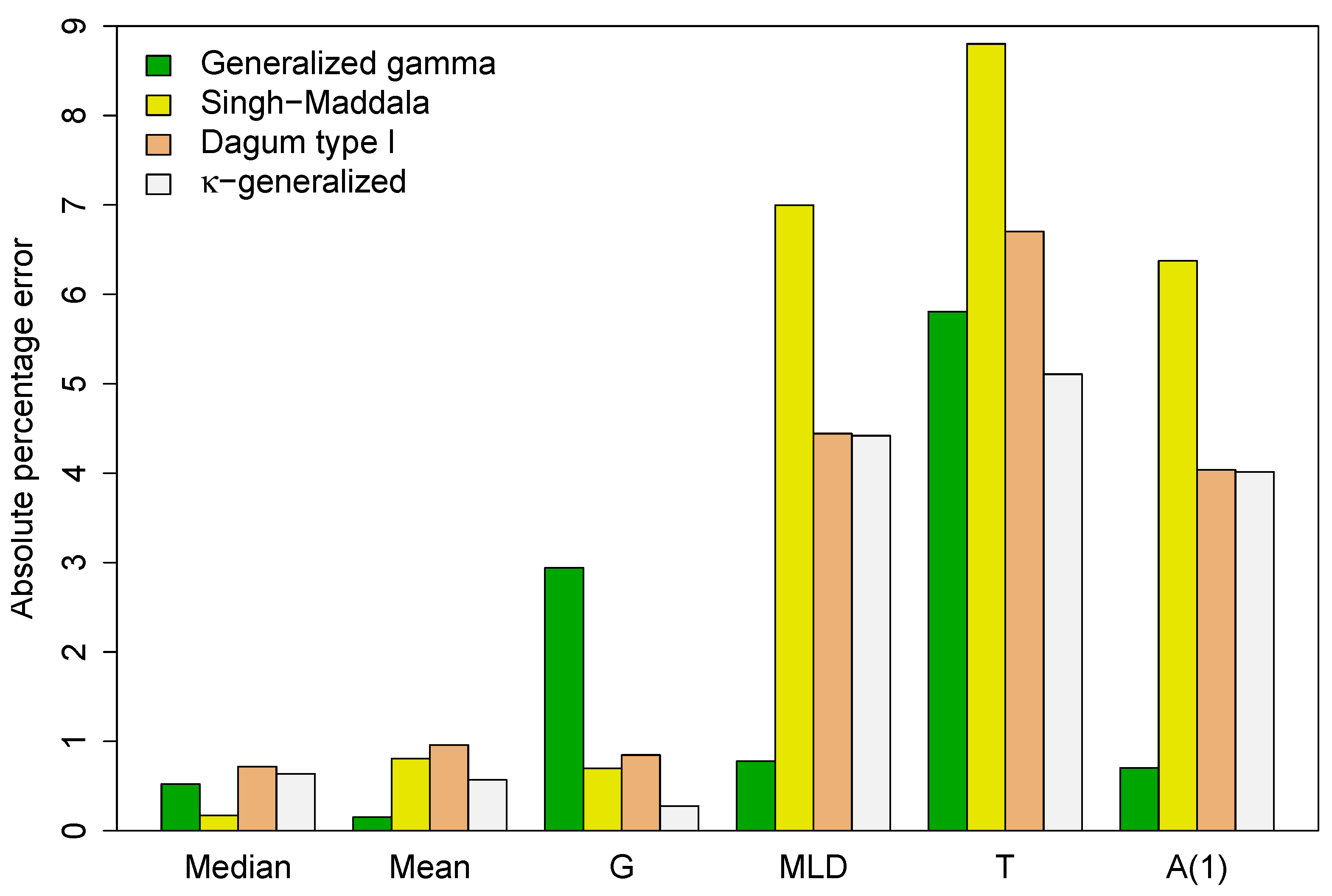
For each of the models examined, the accuracy of the implied statistics is evaluated by calculating the absolute percentage error:
between the predicted values (P) and the actual sample estimates (A) given in Table 3. The results are summarized in Figure 4.
Except for the median, the -generalized distribution has more accurate implied estimates of selected distributional statistics than the Singh–Maddala and Dagum type I models, with the Gini coefficient being significantly more accurate. This implies that the -generalized estimation procedure preserves the mean characteristic of the analyzed data and accurately models intra- and/or inter-group variation. Additionally, when considering income differences in different parts of the income distribution, the -generalized provides more accurate estimates than the two competitors of the index, Theil index T and the Atkinson inequality measure . The Gini is an inequality index sensitive to the middle, while the other indices are more sensitive to the top and bottom of the income distribution. These results support the closest approximation to the income distribution found for the -generalized model.
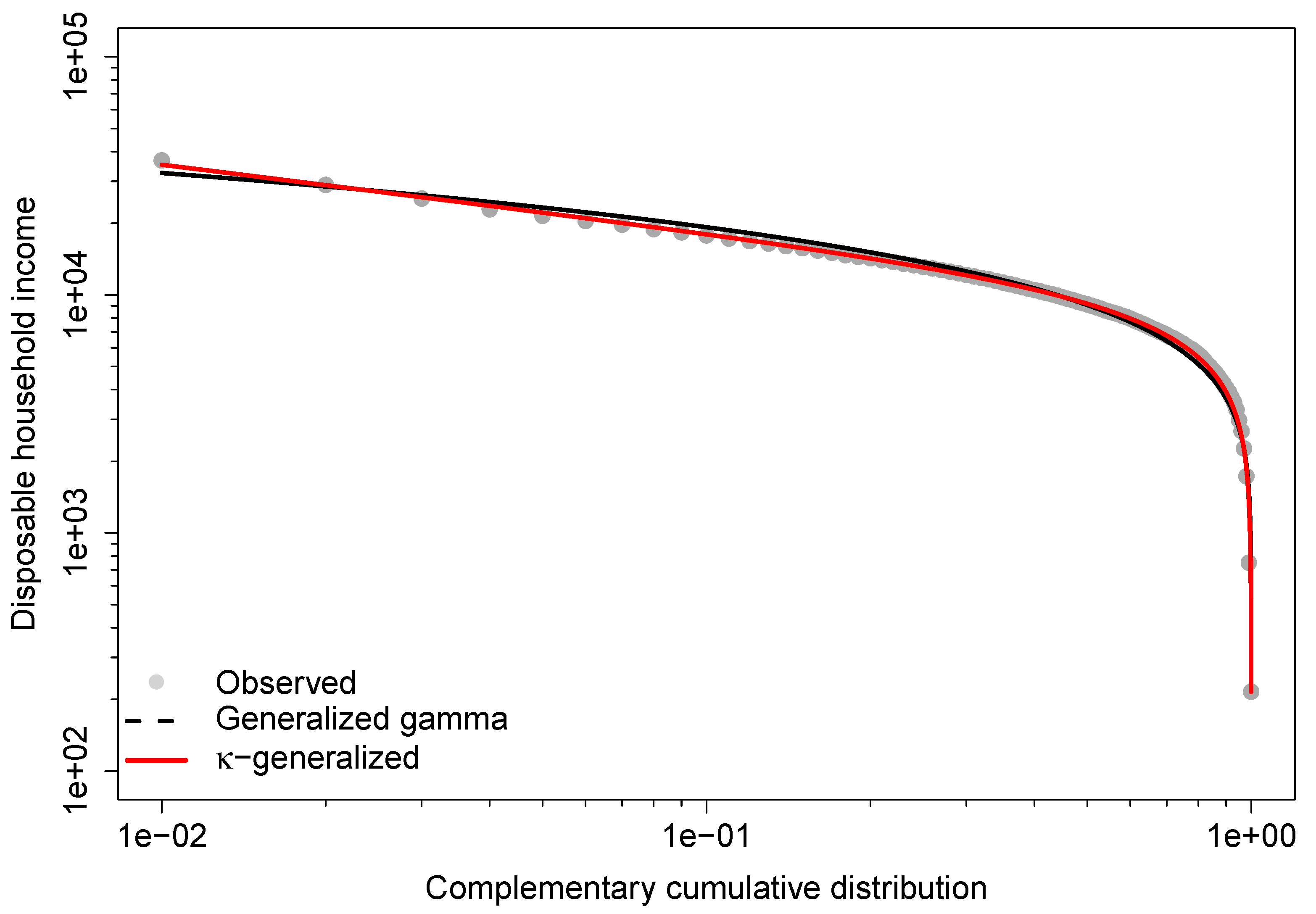
The generalized distribution also outperforms the generalized gamma in predicting the Gini coefficient and Theil index, while the generalized gamma provides more accurate estimates for the index, the measure, the median, and the mean. This agreement is due to better fit in the lower part of the observed distribution, while disagreements arise from poorer fit in the upper-middle range, especially at the top end. This is demonstrated by the double-logarithmic plot in Figure 5, known as the Zipf plot, which shows the relationship between income and the complementary CDF of income for the data under study.
The Zipf plot is natural to use when looking at the upper part of the distribution because it puts more emphasis on the upper tail and makes it easier to detect deviations in that part of the distribution from what a model would predict [97]. The lines show the Zipf plots that were predicted by fitting the generalized gamma and -generalized models. As the graph shows, both are pretty close to the actual data in the lower part of the income distribution. However, the empirical observations of the upper tail are very different from what the generalized gamma says they should be, while the theoretical Zipf plot for the -generalized distribution is much closer to the empirical one in the same part of the observed income distribution.
4. Applications of -Generalized Models to Income and Wealth Data
Apart from the one considered in this review, there have been numerous applications of the -generalized model to real-world income data over the past two decades.
The first study was conducted by [47], who analyzed 2001–2002 household incomes in Germany, Italy, and the United Kingdom. They found excellent agreement between the model and the empirical distributions across the full spectrum of incomes, including the intermediate income range where clear deviation was found when the Weibull model and pure Pareto law were used for interpolation.
The -generalized distribution was later applied to Australian household incomes in 2002–2003 [56] and US family incomes in 2003 [56,57]. The model again described the entire income range well and accurately estimated the inequality level in both countries using the Lorenz curve and Gini measure.
Comparative studies that fit multiple distributions to the same data are crucial for comparing performance. For example, Ref. [58], which examined the distribution of household income in Italy from 1989 to 2006, showed that the -generalized model outperforms three-parameter competitors such as the Singh–Maddala and Dagum type I distributions, except for the GB2, which has an extra parameter. The model has also also been used to analyze household income data for Germany between 1984 and 2007, the United Kingdom between 1991 and 2004, and the United States between 1980 and 2005. In many cases, the distribution of household income is observed to conform to the -generalized model, rather than the Singh–Maddala or Dagum type I distributions. In particular, the -generalized distribution is found to outperform competitors in the right tail of the data. The three-parameter -generalized model provides superior income inequality estimates even when the fit is worse than distributions belonging to the GB2 family, as obtained by [98] when comparing US and Italian income data for the 2000s. Finally, Ref. [60] finds that the -generalized distribution offers a superior fit to the data and, in many cases, estimates income inequality more accurately than alternatives using household income data for 45 countries from Wave IV to Wave IX of the LIS database. (Four-parameter extensions of the -generalized distribution, called extended κ-generalized distributions of the first and second kind—EG1 and EG2, respectively—were introduced by [74]. These two extensions are not discussed here, but Refs. [60,61,74] provide formulas for the moments, Lorenz curve, Gini index, coefficient of variation, mean logarithmic deviation, and Theil index for both the models. The new variants of the -generalized distribution outperform other four-parameter models in almost all cases, especially in estimating inequality indices with greater precision. In addition, a -deformation of the generalized gamma distribution with a power-law tail has recently been proposed by [99], to which the reader is referred for further details.)
The -generalized distribution has also been used to analyze the singularities of survey data on net wealth, which is gross wealth minus total debt [60,61,100]. These data show highly significant frequencies of households or individuals with wealth that is either null or negative. The -generalized model of wealth distribution is a mixture of an atomic and two continuous distributions. The atomic distribution accounts for economic units with no net worth, while a Weibull function accounts for negative net worth data. Positive net worth values, on the other hand, are represented by the -generalized model (3). The -generalized mixture model for wealth distribution was used to model US net worth data from 1984 to 2011 [100]. The model was generally accurate and its performance was superior to that of finite mixture models based on the Singh–Maddala and Dagum type I distributions for positive net worth values. Similar results were later obtained by Ref. [60] when analyzing net wealth data for nine countries selected from the Luxembourg Wealth Study (LWS) database. (The Luxembourg Wealth Study database—see https://www.lisdatacenter.org/our-data/lws-database/, accessed on 26 June 2023—is a collaborative project to assemble existing microdata on household wealth into a coherent database, aiming to do for wealth what the LIS database has achieved for income. The LWS was officially launched in 2004 and currently provides wealth data sets for several countries and years).
5. Concluding Remarks
The -generalized distribution, a statistical model developed over several years of collaborative, multidisciplinary research, is a valuable tool for studying income and wealth distributions. This article discussed its basic properties, relationships with other distributions, and important extensions. It also discussed common inequality measures such as the Lorenz curve and Gini index, and how they can be computed from -generalized parameter estimates. A review of empirical applications showed excellent agreement with observed data. It is hoped that the collection of all these results in a single source will facilitate and promote the use of the -generalized distribution.
Funding
This research received no external funding.
Institutional Review Board Statement
Not applicable.
Informed Consent Statement
Not applicable.
Data Availability Statement
The Luxembourg Income Study Database (https://www.lisdatacenter.org/, accessed on 26 June 2023) provides remote access to the microdata through a web-based Job Submission Interface (LISSY). Users have to register to the platform and submit through the LISSY interface their statistical programs written in R, SAS, SPSS or Stata. Data analysis was performed using Stata software version 17 [101] while graphs were generated using R software version 4.3.1 [102]. To allow reproduction of the analysis, software code used in this article is available from the author on request.
Acknowledgments
The author would like to thank the anonymous referees whose comments and suggestions made it possible to improve this paper greatly.
Conflicts of Interest
The author declares no conflict of interest.
References
- Chatterjee, A.; Yarlagadda, S.; Chakrabarti, B.K. Econophysics of Wealth Distributions; Springer: Milano, Italia, 2005. [Google Scholar]
- Yakovenko, V.M. Econophysics, statistical mechanics approach to. In Encyclopedia of Complexity and Systems Science; Meyers, R.A., Ed.; Springer: New York, NY, USA, 2009; pp. 2800–2826. [Google Scholar]
- Yakovenko, V.M.; Rosser, J.B. Colloquium: Statistical mechanics money, wealth, income. Rev. Mod. Phys. 2009, 81, 1703–1725. [Google Scholar] [CrossRef] [Green Version]
- Chakrabarti, B.K.; Chakraborti, A.; Chakravarty, S.R.; Chatterjee, A. Econophysics of Income and Wealth Distributions; Cambridge University Press: New York, NY, USA, 2013. [Google Scholar]
- Milanovic, B. The Haves and the Have-Nots: A Brief and Idiosyncratic History of Global Inequality; Basic Books: New York, NY, USA, 2011. [Google Scholar]
- Stiglitz, J.E. The Price of Inequality: How Today’s Divided Society Endangers Our Future; W. W. Norton & Company: New York, NY, USA, 2012. [Google Scholar]
- Piketty, T. Capital in the Twenty-First Century; The Belknap Press of Harvard University Press: Cambridge, MA, USA, 2014. [Google Scholar]
- Atkinson, A.B. Inequality: What Can Be Done? Harvard University Press: Cambridge, MA, USA, 2015. [Google Scholar]
- Stiglitz, J.E. The Great Divide: Unequal Societies and What We Can Do about Them; W. W. Norton & Company: New York, NY, USA, 2015. [Google Scholar]
- Pareto, V. La legge della domanda. G. Degli Econ. 1895, 10, 59–68. [Google Scholar]
- Pareto, V. La courbe de la répartition de la richesse. In Recueil Publié par la Faculté de Droit à l’Occasion de l’Exposition Nationale Suisse; Viret-Genton, C., Ed.; Université de Lausanne: Lausanne, Switerland, 1896; pp. 373–387. [Google Scholar]
- Pareto, V. Cours d’Économie Politique; Macmillan: London, UK, 1897. [Google Scholar]
- Pareto, V. Aggiunta allo studio della curva delle entrate. G. Degli Econ. 1897, 14, 15–26. [Google Scholar]
- Montroll, E.W.; Shlesinger, M.F. On 1/f noise and other distributions with long tails. Proc. Natl. Acad. Sci. USA 1982, 79, 3380–3383. [Google Scholar] [CrossRef] [PubMed]
- Montroll, E.W.; Shlesinger, M.F. Maximum entropy formalism, fractals, scaling phenomena, and 1/f noise: A tale of tails. J. Stat. Phys. 1983, 32, 209–230. [Google Scholar] [CrossRef]
- Drăgulescu, A.; Yakovenko, V.M. Evidence for the exponential distribution of income in the USA. Eur. Phys. J. B 2001, 20, 585–589. [Google Scholar] [CrossRef] [Green Version]
- Drăgulescu, A.; Yakovenko, V.M. Exponential and power-law probability distributions of wealth and income in the United Kingdom and the United States. Phys. A Stat. Mech. Its Appl. 2001, 299, 213–221. [Google Scholar] [CrossRef] [Green Version]
- Souma, W. Universal structure of the personal income distribution. Fractals 2001, 9, 463–470. [Google Scholar] [CrossRef] [Green Version]
- Clementi, F.; Gallegati, M. Power law tails in the Italian personal income distribution. Phys. A Stat. Mech. Its Appl. 2005, 350, 427–438. [Google Scholar] [CrossRef] [Green Version]
- Clementi, F.; Gallegati, M. Pareto’s law of income distribution: Evidence for Germany, the United Kingdom, and the United States. In Econophysics of Wealth Distributions; Chatterjee, A., Yarlagadda, S., Chakrabarti, B.K., Eds.; Springer: Milan, Italy, 2005; pp. 3–14. [Google Scholar]
- Silva, A.C.; Yakovenko, V.M. Temporal evolution of the “thermal” and “superthermal” income classes in the USA during 1983–2001. Europhys. Lett. 2005, 69, 304–310. [Google Scholar] [CrossRef] [Green Version]
- Nirei, M.; Souma, W. A two factor model of income distribution dynamics. Rev. Income Wealth 2007, 53, 440–459. [Google Scholar] [CrossRef]
- Gibrat, R. Les Inégalités économiques. Applications: Aux Inégalités des Richesses, à la Concentration des Entreprises, aux Population des Villes, aux Statistiques des Familles, etc., d’une loi Nouvelle: La loi de l’Effet Proportionnel; Librairie du Recueil Sirey: Paris, France, 1931. [Google Scholar]
- Salem, A.B.Z.; Mount, T.D. A convenient descriptive model of income distribution: The gamma density. Econometrica 1974, 42, 1115–1127. [Google Scholar] [CrossRef]
- Aitchison, J.; Brown, J.A.C. On criteria for descriptions of income distribuition. Metroeconomica 1954, 6, 88–107. [Google Scholar] [CrossRef]
- Aitchison, J.; Brown, J.A.C. The Lognormal Distribution with Special Reference to Its Use in Economics; Cambridge University Press: New York, NY, USA, 1957. [Google Scholar]
- McDonald, J.B.; Ransom, M.R. Functional forms, estimation techniques and the distribution of income. Econometrica 1979, 47, 1513–1525. [Google Scholar] [CrossRef]
- Majumder, A.; Chakravarty, S.R. Distribution of personal income: Development of a new model and its application to U. S. income aata. J. Appl. Econom. 1990, 5, 189–196. [Google Scholar] [CrossRef]
- Atoda, N.; Suruga, T.; Tachibanaki, T. Statistical inference of functional forms for income distribution. Econ. Stud. Q. 1988, 39, 14–40. [Google Scholar]
- Esteban, J.M. Income-share elasticity and the size distribution of income. Int. Econ. Rev. 1986, 27, 439–444. [Google Scholar] [CrossRef]
- Kloek, T.; van Dijk, H.K. Efficient estimation of income distribution parameters. J. Econom. 1978, 8, 61–74. [Google Scholar] [CrossRef] [Green Version]
- Taillie, C. Lorenz ordering within the generalized gamma family of income distributions. In Statistical Distributions in Scientific Work; Taillie, C., Patil, G.P., Baldessari, B.A., Eds.; D. Reidel Publishing Company: Dordrecht, The Netherlands, 1981; Volume 6, pp. 181–192. [Google Scholar]
- Singh, S.K.; Maddala, G.S. A function for size distribution of incomes. Econometrica 1976, 44, 963–970. [Google Scholar] [CrossRef]
- Dagum, C. A new model of personal income distribution: Specification and estimation. Econ. Appliquée 1977, 30, 413–436. [Google Scholar]
- McDonald, J.B. Some generalized functions for the size distribution of income. Econometrica 1984, 52, 647–665. [Google Scholar] [CrossRef]
- Reed, W.J.; Jorgensen, M. The double Pareto-lognormal distribution—A new parametric model for size distributions. Commun. Stat.-Theory Methods 2004, 33, 1733–1753. [Google Scholar] [CrossRef]
- McDonald, J.B.; Xu, Y.J. A generalization of the beta distribution with applications. J. Econom. 1995, 66, 133–152. [Google Scholar] [CrossRef]
- Reed, W.J. Brownian-Laplace motion and its use in financial modelling. Commun. Stat. Theory Methods 2007, 36, 473–484. [Google Scholar] [CrossRef] [Green Version]
- McDonald, J.B.; Ransom, M.R. The generalized beta distribution as a model for the distribution of income: Estimation of related measures of Inequality. In Modeling Income Distributions and Lorenz Curves; Chotikapanich, D., Ed.; Springer: New York, NY, USA, 2008; pp. 147–166. [Google Scholar]
- Reed, W.J.; Wu, F. New four- and five-parameter models for income distributions. In Modeling Income Distributions and Lorenz Curves; Chotikapanich, D., Ed.; Springer: New York, NY, USA, 2008; pp. 211–223. [Google Scholar]
- Kaniadakis, G. Non-linear kinetics underlying generalized statistics. Phys. A Stat. Mech. Its Appl. 2001, 296, 405–425. [Google Scholar] [CrossRef] [Green Version]
- Kaniadakis, G. Statistical mechanics in the context of special relativity. Phys. Rev. E 2002, 66, 056125. [Google Scholar] [CrossRef] [PubMed] [Green Version]
- Kaniadakis, G. Statistical mechanics in the context of special relativity. II. Phys. Rev. E 2005, 72, 036108. [Google Scholar] [CrossRef] [PubMed] [Green Version]
- Kaniadakis, G. Maximum entropy principle and power-law tailed distributions. Eur. Phys. J. B 2009, 70, 3–13. [Google Scholar] [CrossRef] [Green Version]
- Kaniadakis, G. Relativistic entropy and related Boltzmann kinetics. Eur. Phys. J. A 2009, 40, 275–287. [Google Scholar] [CrossRef] [Green Version]
- Kaniadakis, G. Theoretical foundations and mathematical formalism of the power-law tailed statistical distributions. Entropy 2013, 15, 3983–4010. [Google Scholar] [CrossRef] [Green Version]
- Clementi, F.; Gallegati, M.; Kaniadakis, G. κ-generalized statistics in personal income distribution. Eur. Phys. J. B 2007, 57, 187–193. [Google Scholar] [CrossRef] [Green Version]
- Rajaonarison, D.; Bolduc, D.; Jayet, H. The K-deformed multinomial logit model. Econ. Lett. 2005, 86, 13–20. [Google Scholar] [CrossRef]
- Rajaonarison, D. Deterministic heterogeneity in tastes and product differentiation in the K-logit model. Econ. Lett. 2008, 100, 396–398. [Google Scholar] [CrossRef]
- Trivellato, B. Replication and shortfall risk in a binomial model with transaction costs. Math. Methods Oper. Res. 2009, 69, 1–26. [Google Scholar] [CrossRef]
- Imparato, D.; Trivellato, B. Geometry of extended exponential models. In Algebraic and Geometric Methods in Statistics; Gibilisco, P., Riccomagno, E., Pistone, G., Wynn, H.P., Eds.; Cambridge University Press: Cambridge, UK, 2009; pp. 307–326. [Google Scholar]
- Trivellato, B. The minimal κ-entropy martingale measure. Int. J. Theor. Appl. Financ. 2012, 15, 1250038. [Google Scholar] [CrossRef]
- Trivellato, B. Deformed exponentials and applications to finance. Entropy 2013, 15, 3471–3489. [Google Scholar] [CrossRef] [Green Version]
- Moretto, E.; Pasquali, S.; Trivellato, B. Option pricing under deformed Gaussian distributions. Phys. A Stat. Mech. Appl. 2016, 446, 246–263. [Google Scholar] [CrossRef]
- Moretto, E.; Pasquali, S.; Trivellato, B. A non-Gaussian option pricing model based on Kaniadakis exponential deformation. Eur. Phys. J. B 2017, 90, 179. [Google Scholar] [CrossRef]
- Clementi, F.; Di Matteo, T.; Gallegati, M.; Kaniadakis, G. The κ-generalized distribution: A new descriptive model for the size distribution of incomes. Phys. A Stat. Mech. Appl. 2008, 387, 3201–3208. [Google Scholar] [CrossRef] [Green Version]
- Clementi, F.; Gallegati, M.; Kaniadakis, G. A κ-generalized statistical mechanics approach to income analysis. J. Stat. Mech. Theory Exp. 2009, 2009, P02037. [Google Scholar] [CrossRef] [Green Version]
- Clementi, F.; Gallegati, M.; Kaniadakis, G. A model of personal income distribution with application to Italian data. Empir. Econ. 2010, 39, 559–591. [Google Scholar] [CrossRef]
- Clementi, F.; Gallegati, M.; Kaniadakis, G. A new model of income distribution: The κ-generalized distribution. J. Econ. 2012, 105, 63–91. [Google Scholar] [CrossRef] [Green Version]
- Clementi, F.; Gallegati, M. The Distribution of Income and Wealth: Parametric Modeling with the κ-Generalized Family; Springer International Publishing AG: Cham, Switerland, 2016. [Google Scholar]
- Clementi, F.; Gallegati, M.; Kaniadakis, G.; Landini, S. κ-generalized models of income and wealth distributions: A survey. Eur. Phys. J. Spec. Top. 2016, 225, 1959–1984. [Google Scholar] [CrossRef] [Green Version]
- Clementi, F.; Gallegati, M. New economic windows on income and wealth: The κ-generalized family of distributions. J. Soc. Econ. Stat. 2017, 6, 1–15. [Google Scholar]
- Landini, S. Mathematics of strange quantities: Why are κ-generalized models a good fit to income and wealth distributions? An explanation. In The Distribution of Income and Wealth: Parametric Modeling with the κ-Generalized Family; Clementi, F., Gallegati, M., Eds.; Springer International Publishing AG: Cham, Switerland, 2016; pp. 93–132. [Google Scholar]
- Bartels, C.P.A.; van Metelen, H. Alternative Probability Density Functions of Income: A Comparison of the Longnormal-, Gamma- and Weibull-Distribution with Dutch Data; Research Memorandum 29; Department of Quantitative Studies, Faculty of Economics, Vrije Universiteit: Amsterdam, The Netherlands, 1975. [Google Scholar]
- Bartels, C.P.A. Economic Aspects of Regional Welfare: Income Distribution and Unemployment; Martinus Nijhoff: Leiden, The Netherlands, 1977. [Google Scholar]
- Espinguet, P.; Terraza, M. Essai d’extrapolation des distributions de salaires français. Econ. Appliquée 1983, 36, 535–561. [Google Scholar]
- Bordley, R.F.; McDonald, J.B.; Mantrala, A. Something new, something old: Parametric models for the size distribution of income. J. Income Distrib. 1996, 6, 91–103. [Google Scholar] [CrossRef]
- Brachmann, K.; Stich, A.; Trede, M. Evaluating parametric income distribution models. Allg. Stat. Arch. 1996, 80, 285–298. [Google Scholar]
- Tachibanaki, T.; Suruga, T.; Atoda, N. Estimations of income distribution parameters for individual observations by maximum likelihood method. J. Jpn. Stat. Soc. 1997, 27, 191–203. [Google Scholar] [CrossRef] [Green Version]
- Mandelbrot, B. The Pareto-Lévy law and the distribution of income. Int. Econ. Rev. 1960, 1, 79–106. [Google Scholar] [CrossRef] [Green Version]
- Kakwani, N. Income Inequality and Poverty: Methods of Estimation and Policy Applications; Oxford University Press: New York, NY, USA, 1980. [Google Scholar]
- Lorenz, M.O. Methods of measuring the concentration of wealth. Publ. Am. Stat. Assoc. 1905, 9, 209–219. [Google Scholar]
- Gastwirth, J.L. A general definition of the Lorenz curve. Econometrica 1971, 39, 1037–1039. [Google Scholar] [CrossRef]
- Okamoto, M. Extension of the κ-Generalized Distribution: New Four-Parameter Models for the Size Distribution of Income and Consumption; Working Paper 600; LIS Cross-National Data Center: Luxembourg, 2013; Available online: https://www.lisdatacenter.org/wps/liswps/600.pdf (accessed on 26 June 2023).
- Gini, C. Sulla misura della concentrazione e della variabilità dei caratteri. Atti Del R. Ist. Veneto Di Sci. Lett. Ed Arti 1914, 73, 1201–1248. [Google Scholar]
- Arnold, B.C.; Laguna, L. On Generalized Pareto Distributions with Applications to Income Data; Iowa State University Press: Ames, IA, USA, 1977. [Google Scholar]
- Kleiber, C.; Kotz, S. Statistical Size Distributions in Economics and Actuarial Sciences; John Wiley & Sons: New York, NY, USA, 2003. [Google Scholar]
- Allison, P.D. Measures of inequality. Am. Sociol. Rev. 1978, 43, 865–880. [Google Scholar] [CrossRef]
- Cowell, F.A. Generalized entropy and the measurement of distributional change. Eur. Econ. Rev. 1980, 13, 147–159. [Google Scholar] [CrossRef]
- Cowell, F.A. On the structure of additive inequality measures. Rev. Econ. Stud. 1980, 47, 521–531. [Google Scholar] [CrossRef]
- Shorrocks, A.F. The class of additively decomposable inequality measures. Econometrica 1980, 48, 613–625. [Google Scholar] [CrossRef] [Green Version]
- Cowell, F.A.; Kuga, K. Additivity and the entropy concept: An axiomatic approach to inequality measurement. J. Econ. Theory 1981, 25, 131–143. [Google Scholar] [CrossRef]
- Cowell, F.A.; Kuga, K. Inequality measurement: An axiomatic approach. Eur. Econ. Rev. 1981, 15, 287–305. [Google Scholar] [CrossRef]
- Theil, H. Economics and Information Theory; North-Holland: Amsterdam, The Netherlands, 1967. [Google Scholar]
- Sarabia, J.M.; Jordá, V.; Remuzgo, L. The Theil indices in parametric families of income distributions—A short review. Rev. Income Wealth 2017, 63, 867–880. [Google Scholar] [CrossRef]
- Atkinson, A.B. On the measurement of inequality. J. Econ. Theory 1970, 2, 244–263. [Google Scholar] [CrossRef]
- Jenkins, S.P. Distributionally-sensitive inequality indices and the GB2 income distribution. Rev. Income Wealth 2009, 55, 392–398. [Google Scholar] [CrossRef]
- Cowell, F.A. Measuring Inequality; Oxford University Press: New York, NY, USA, 2011. [Google Scholar]
- Kleiber, C. The existence of population inequality measures. Econ. Lett. 1997, 57, 39–44. [Google Scholar] [CrossRef]
- Rao, C. Linear Statistical Inference and Its Applications; John Wiley & Sons: New York, NY, USA, 1973. [Google Scholar]
- Ghosh, J.K. Higher Order Asymptotics; Institute of Mathematical Statistics and American Statistical Association: Hayward, CA, USA, 1994. [Google Scholar]
- Araar, A.; Duclos, J.Y. User Manual for Stata Package DASP: Version 3.0; PEP, World Bank, UNDP and Université Laval, 2022. Available online: http://dasp.ecn.ulaval.ca/dasp3/manual/DASP_MANUAL_V303.pdf (accessed on 26 June 2023).
- Stacy, E.W. A generalization of the gamma distribution. Ann. Math. Stat. 1962, 33, 1187–1192. [Google Scholar] [CrossRef]
- Chotikapanich, D.; Griffiths, W.; Hajargasht, G.; Karunarathne, W.; Rao, D. Using the GB2 income distribution. Econometrics 2018, 6, 21. [Google Scholar] [CrossRef] [Green Version]
- Jordá, V.; Alonso, J.M. New estimates on educational attainment using a continuous approach (1970–2010). World Dev. 2017, 90, 281–293. [Google Scholar] [CrossRef] [Green Version]
- Fellman, J. Estimation of Gini coefficients using Lorenz curves. J. Stat. Econom. Methods 2012, 1, 31–38. [Google Scholar]
- Takayasu, H. Fractals in Physical Science; Manchester University Press: Manchester, UK, 1991. [Google Scholar]
- Okamoto, M. Evaluation of the goodness of fit of new statistical size distributions with consideration of accurate income inequality estimation. Econ. Bull. 2012, 32, 2969–2982. [Google Scholar]
- Vallejos, A.; Ormazábal, I.; Borotto, F.A.; Astudillo, H.F. A new κ-deformed parametric model for the size distribution of wealth. Phys. Stat. Mech. Appl. 2019, 514, 819–829. [Google Scholar] [CrossRef] [Green Version]
- Clementi, F.; Gallegati, M.; Kaniadakis, G. A generalized statistical model for the size distribution of wealth. J. Stat. Mech. Theory Exp. 2012, 2012, P12006. [Google Scholar] [CrossRef] [Green Version]
- StataCorp. Stata Statistical Software: Release 17; StataCorp: College Station, TX, USA, 2021; Available online: https://www.stata.com/ (accessed on 26 June 2023).
- R Core Team. R: A Language and Environment for Statistical Computing; R Foundation for Statistical Computing: Vienna, Austria, 2023; Available online: https://www.R-project.org/ (accessed on 26 June 2023).
Figure 1.
-generalized PDF (left) and complementary CDF (right) for different values of the parameters. The complementary CDF is plotted on double-log axes, which is the standard way to emphasize the right-tail behavior of a distribution.
Figure 1.
-generalized PDF (left) and complementary CDF (right) for different values of the parameters. The complementary CDF is plotted on double-log axes, which is the standard way to emphasize the right-tail behavior of a distribution.


Figure 2.
Lorenz curves for two -generalized distributions.

Figure 3.
-generalized distribution fitted to Greek household income data for 2016. The red solid line represents the -generalized model, which fits the data well over the whole range from low to high incomes, including the middle income region. It is compared to the Weibull (blue dashed line) and Pareto power-law (green dashed line) distributions. The complementary cumulative distribution is plotted on double-log axes, emphasizing the right-tail behavior of the distribution. The Lorenz curve plot compares the empirical and theoretical curves, with the gray solid line representing the Lorenz curve of a society with equal income distribution. The Q-Q plot of sample percentiles versus theoretical percentiles of the fitted -generalized shows excellent fit, with corresponding percentiles being close to the line from the origin.

Figure 4.
Absolute percentage error between the predicted values for key distributional summary measures and their sample counterparts.
Figure 4.
Absolute percentage error between the predicted values for key distributional summary measures and their sample counterparts.

Figure 5.
Zipf plot for the 2016 Greek household income data. The lines are the predicted Zipf plots obtained from the fit of the generalized gamma and -generalized models.
Figure 5.
Zipf plot for the 2016 Greek household income data. The lines are the predicted Zipf plots obtained from the fit of the generalized gamma and -generalized models.


Table 1.
Observed and predicted values of the median, the mean, the Gini index G and the Atkinson inequality measure .
Table 1.
Observed and predicted values of the median, the mean, the Gini index G and the Atkinson inequality measure .
| Statistic | Observed | Predicted | ||
|---|---|---|---|---|
| Value | LB a | UB b | ||
| Median | 9123 | 8983 | 9264 | 9181 |
| Mean | 10,548 | 10,292 | 10,805 | 10,488 |
| G | 0.323 | 0.312 | 0.334 | 0.322 |
| 0.179 | 0.169 | 0.189 | 0.172 | |
Notes: lower bound of the 95% normal-based confidence interval obtained by adding −1.96 times the standard error to the sample indicator; upper bound of the 95% normal-based confidence interval obtained by adding times the standard error to the sample indicator. Source: author’s calculations based on Greek LIS data for 2016.
Table 2.
Maximum likelihood estimates for the generalized gamma, Singh–Maddala, Dagum type I and -generalized models of income distribution.
Table 2.
Maximum likelihood estimates for the generalized gamma, Singh–Maddala, Dagum type I and -generalized models of income distribution.
| Model | Parameters | Goodness-of-Fit Criteria | |||||||
|---|---|---|---|---|---|---|---|---|---|
| () | () | , , | |||||||
| GG | 0.684 | 829 | 5.475 | 2.325 | 2.047 | 0.939 | 0.812 | ||
| (0.018) | (115) | (0.270) | |||||||
| SM | 2.441 | 12,531 | 1.835 | 0.716 | 0.574 | 0.319 | 0.187 | ||
| (0.021) | (219) | (0.053) | |||||||
| D | 3.705 | 11,705 | 0.560 | 0.539 | 0.437 | 0.281 | 0.211 | ||
| (0.041) | (104) | (0.011) | |||||||
| -gen | 2.233 | 10,667 | 0.630 | 0.530 | 0.418 | 0.188 | 0.139 | ||
| (0.017) | (46) | (0.014) | |||||||
Notes: GG = generalized gamma, SM = Singh-Maddala, D = Dagum type I, -gen = -generalized; numbers in parentheses: estimated standard errors; = root mean square error, = mean absolute error, = root mean square error between the observed and estimated Lorenz curves, = mean absolute error between the observed and estimated Lorenz curves; values multiplied by 100. Source: author’s calculations based on Greek LIS data for 2016.
Table 3.
Observed and predicted values of selected distributional statistics.
| Statistic a | Observed | Predicted d | |||||||
|---|---|---|---|---|---|---|---|---|---|
| Value | LB b | UB c | GG | SM | D | -gen | |||
| Median | 9123 | 8983 | 9264 | 9076 | 9108 | 9189 | 9181 | ||
| Mean | 10,548 | 10,292 | 10,805 | 10,532 | 10,463 | 10,447 | 10,488 | ||
| G | 0.323 | 0.312 | 0.334 | 0.333 | 0.321 | 0.320 | 0.322 | ||
| 0.197 | 0.185 | 0.209 | 0.196 | 0.183 | 0.188 | 0.188 | |||
| T | 0.191 | 0.175 | 0.207 | 0.180 | 0.174 | 0.178 | 0.181 | ||
| 0.179 | 0.169 | 0.189 | 0.178 | 0.168 | 0.172 | 0.172 | |||
Notes: G = Gini index, = mean logarithmic deviation index, T = Theil index, = Atkinson coefficient with inequality aversion parameter equal to 1; lower bound of the 95% normal-based confidence interval obtained by adding times the standard error to the sample indicator; upper bound of the 95% normal-based confidence interval obtained by adding times the standard error to the sample indicator; GG = generalized gamma, SM = Singh–Maddala, D = Dagum type I, -gen = -generalized. Source: author’s calculations based on Greek LIS data for 2016.
Disclaimer/Publisher’s Note: The statements, opinions and data contained in all publications are solely those of the individual author(s) and contributor(s) and not of MDPI and/or the editor(s). MDPI and/or the editor(s) disclaim responsibility for any injury to people or property resulting from any ideas, methods, instructions or products referred to in the content. |
© 2023 by the author. Licensee MDPI, Basel, Switzerland. This article is an open access article distributed under the terms and conditions of the Creative Commons Attribution (CC BY) license (https://creativecommons.org/licenses/by/4.0/).
Share and Cite
MDPI and ACS Style
Clementi, F. The Kaniadakis Distribution for the Analysis of Income and Wealth Data. Entropy 2023, 25, 1141. https://doi.org/10.3390/e25081141
AMA Style
Clementi F. The Kaniadakis Distribution for the Analysis of Income and Wealth Data. Entropy. 2023; 25(8):1141. https://doi.org/10.3390/e25081141
Chicago/Turabian StyleClementi, Fabio. 2023. "The Kaniadakis Distribution for the Analysis of Income and Wealth Data" Entropy 25, no. 8: 1141. https://doi.org/10.3390/e25081141
Note that from the first issue of 2016, this journal uses article numbers instead of page numbers. See further details here.