

Attention-Based Spatial–Temporal Convolution Gated Recurrent Unit for Traffic Flow Forecasting

Abstract
:1. Introduction
2. Related Work
3. Preliminaries
- (1)
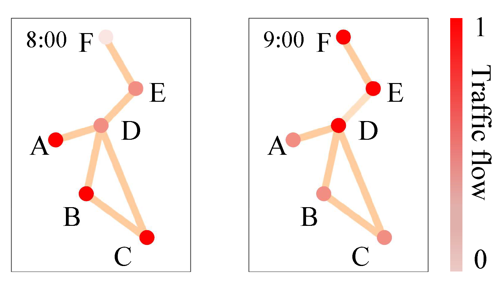
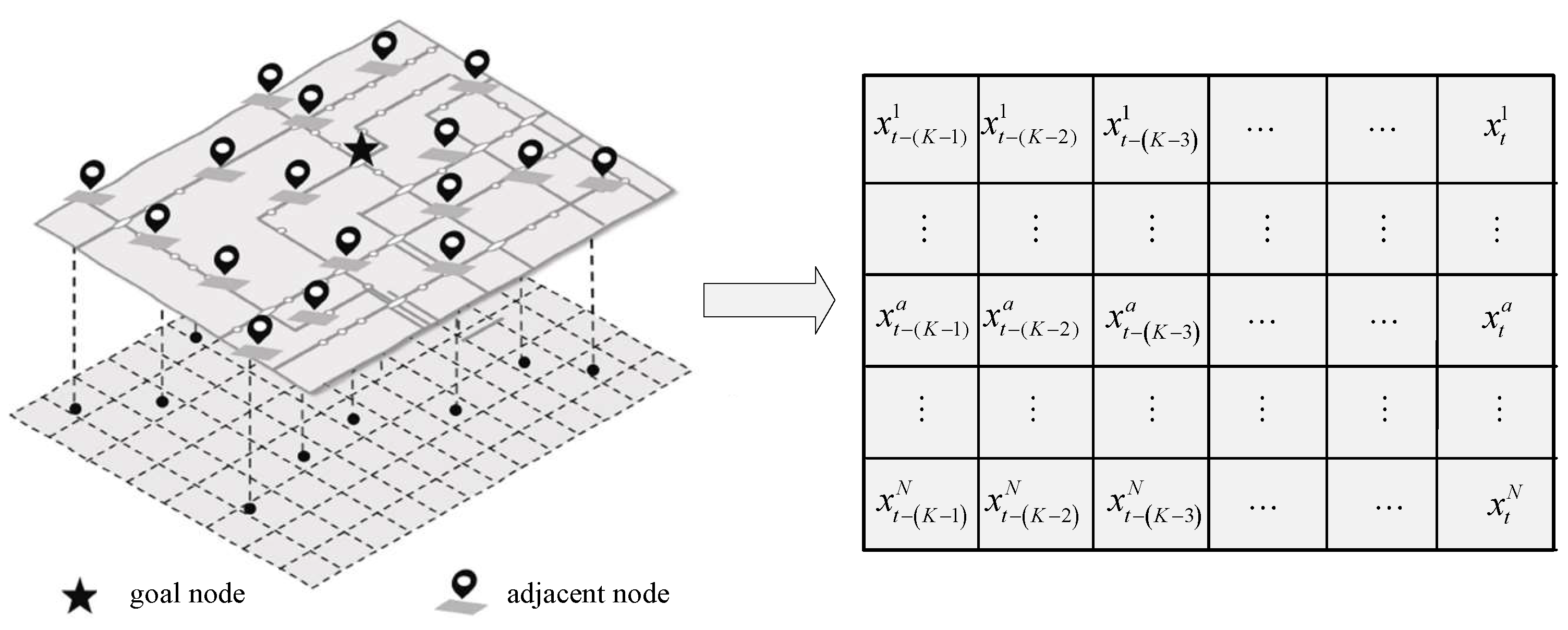
- The plan is divided into a grid based on the relative position of each traffic sensor on the map, so that all the goal nodes and their associated nodes are divided into corresponding small squares, with each small square containing a traffic node.
- (2)
- The traffic flow data recorded by the sensors at these nodes are filled in as pixel values in the small cells.
- (3)
- This city sensor map is converted into a spatial–temporal image of traffic flow with length N squares and width K squares, where the coordinates of the goal node are , where , and the coordinates of the adjacent node are , where .
4. Model Structure
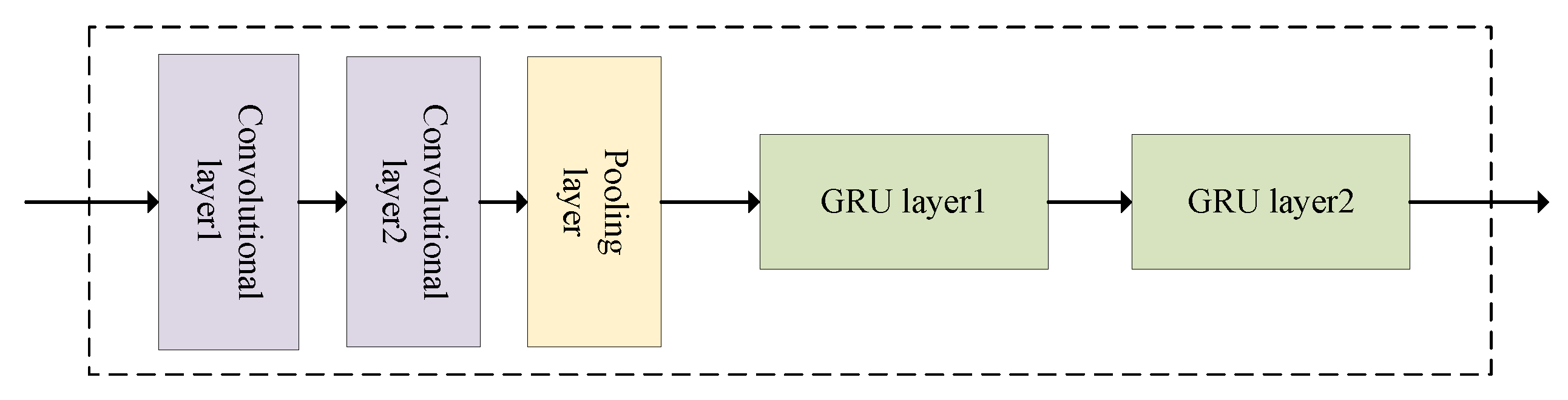
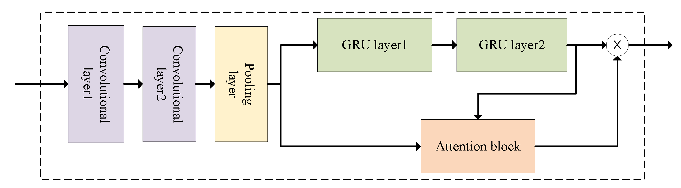
4.1. ConvGRU Module
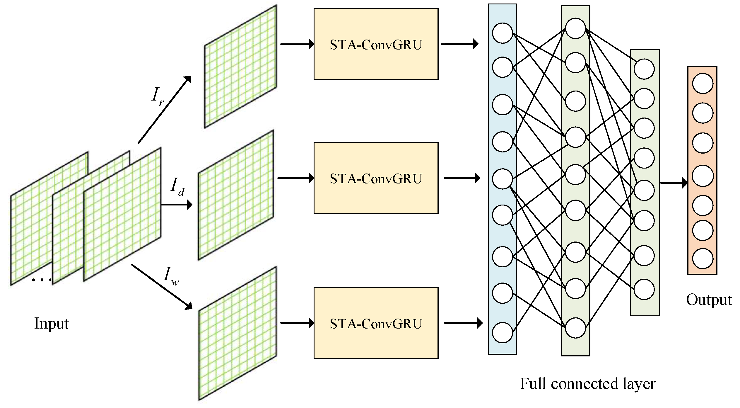
4.2. STA-ConvGRU Module
5. Experiments
5.1. Experimental Setup
5.1.1. Experimental Data
5.1.2. Hyperparameter Settings
5.1.3. Evaluation Metrics
5.1.4. Compared Methods
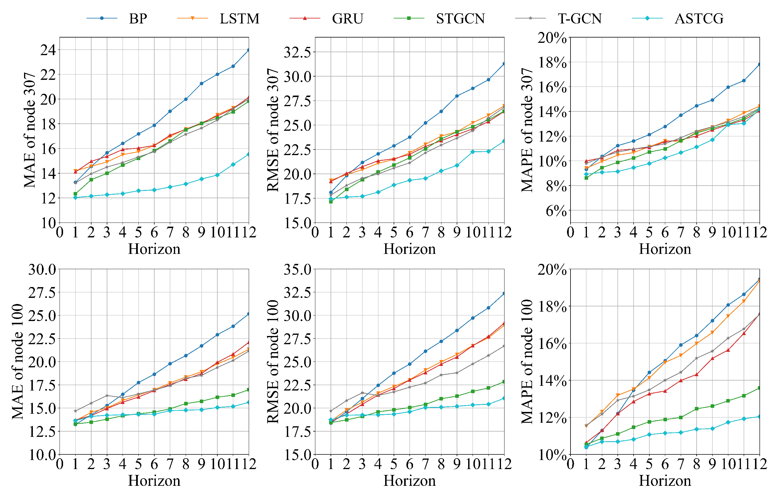
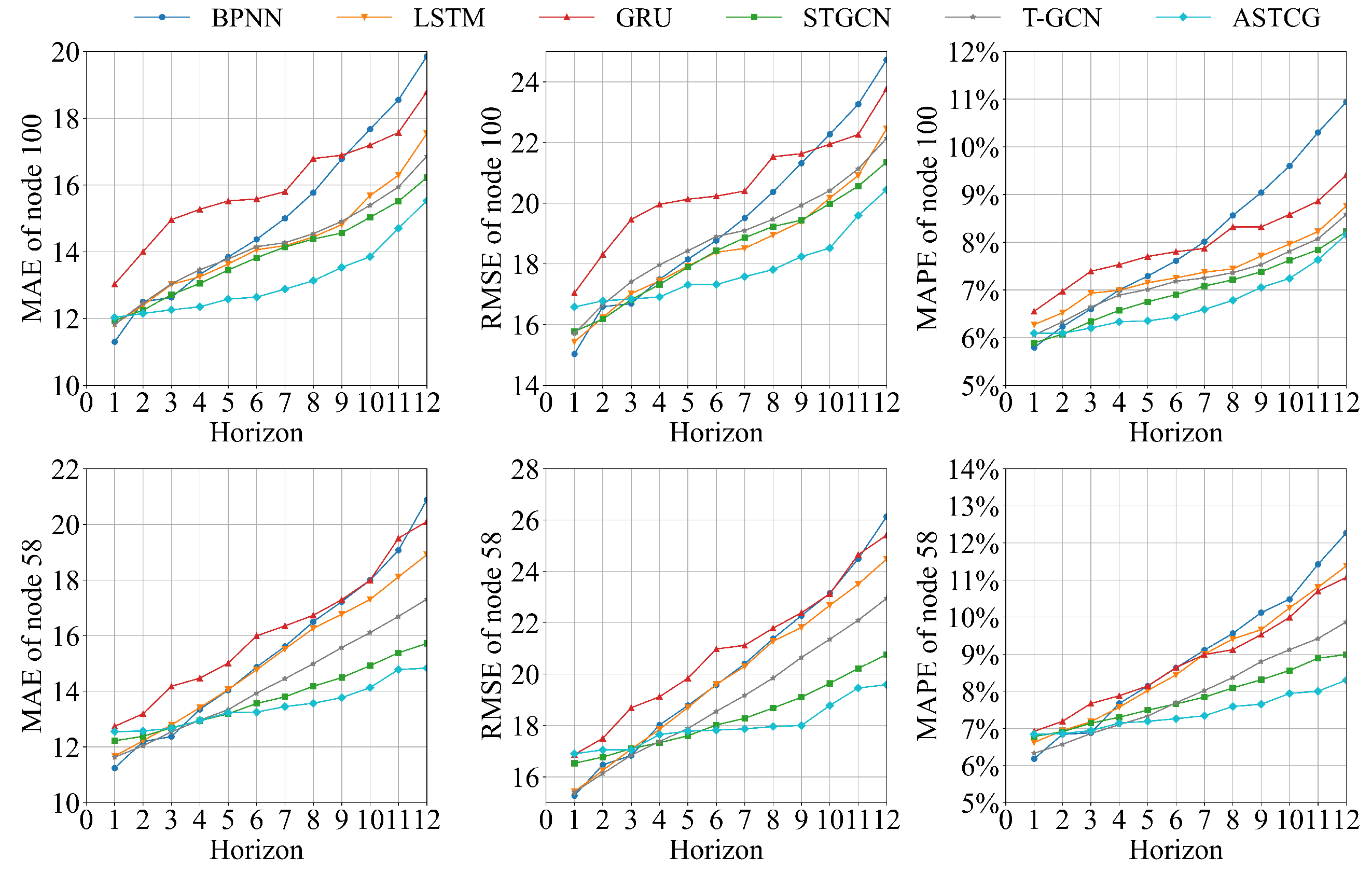
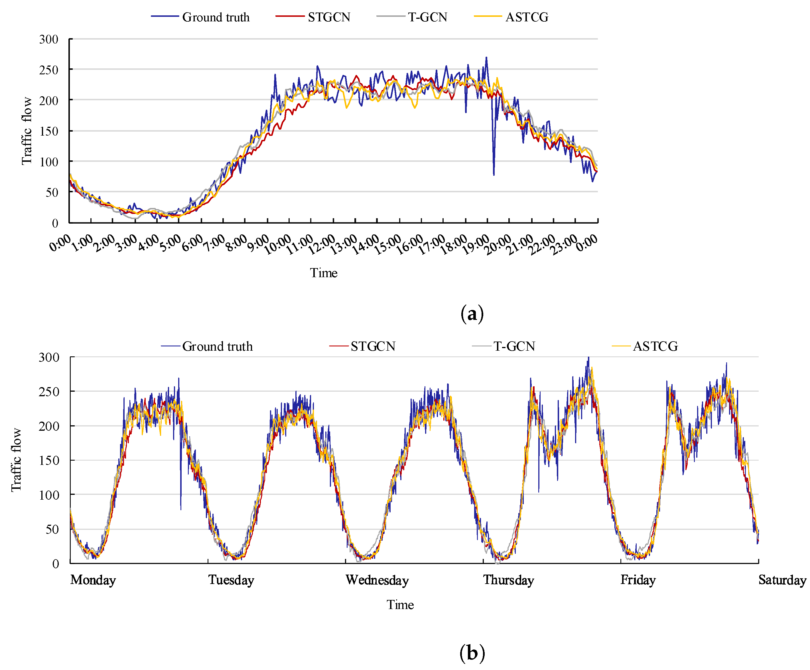
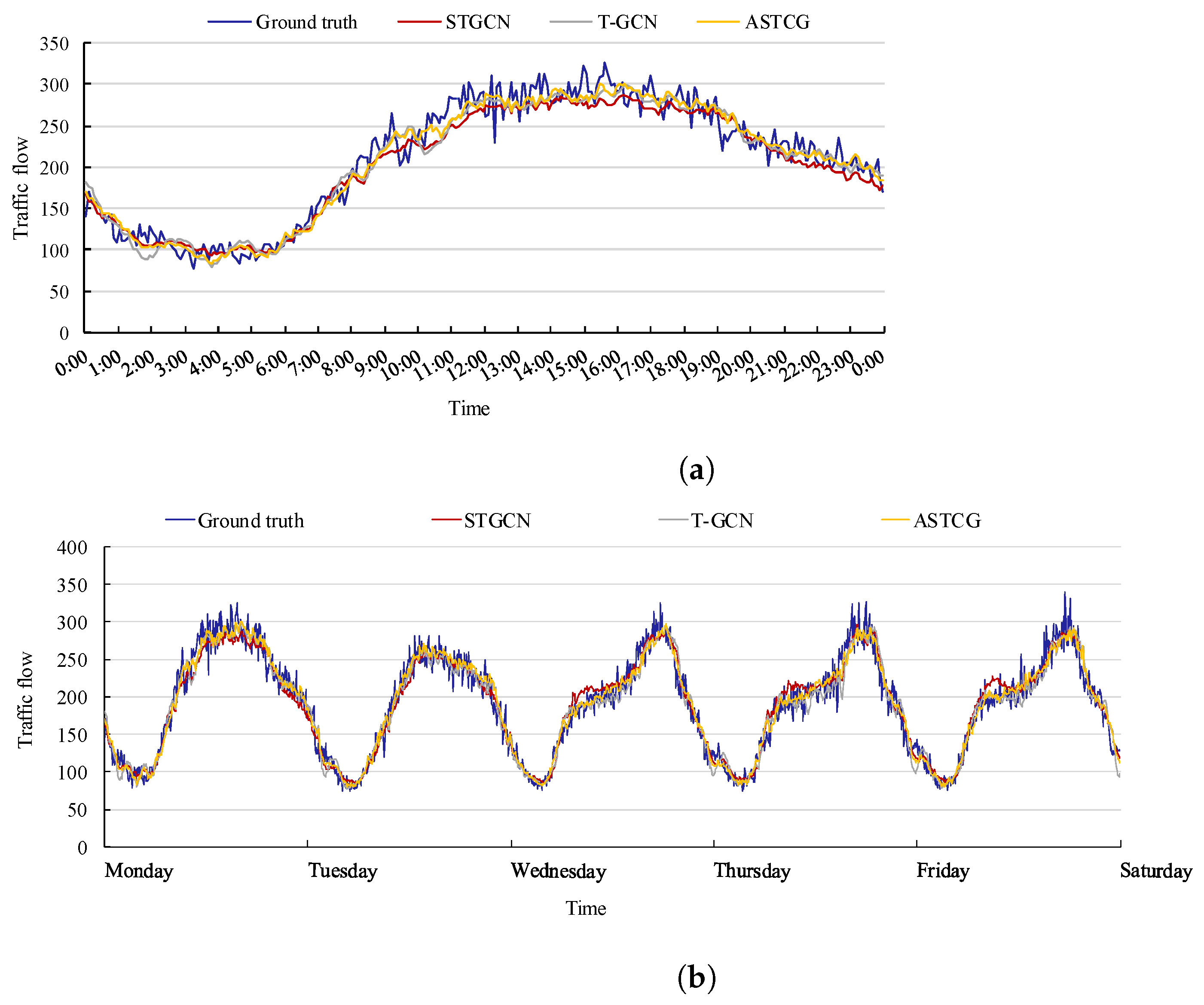
5.2. Experimental Results
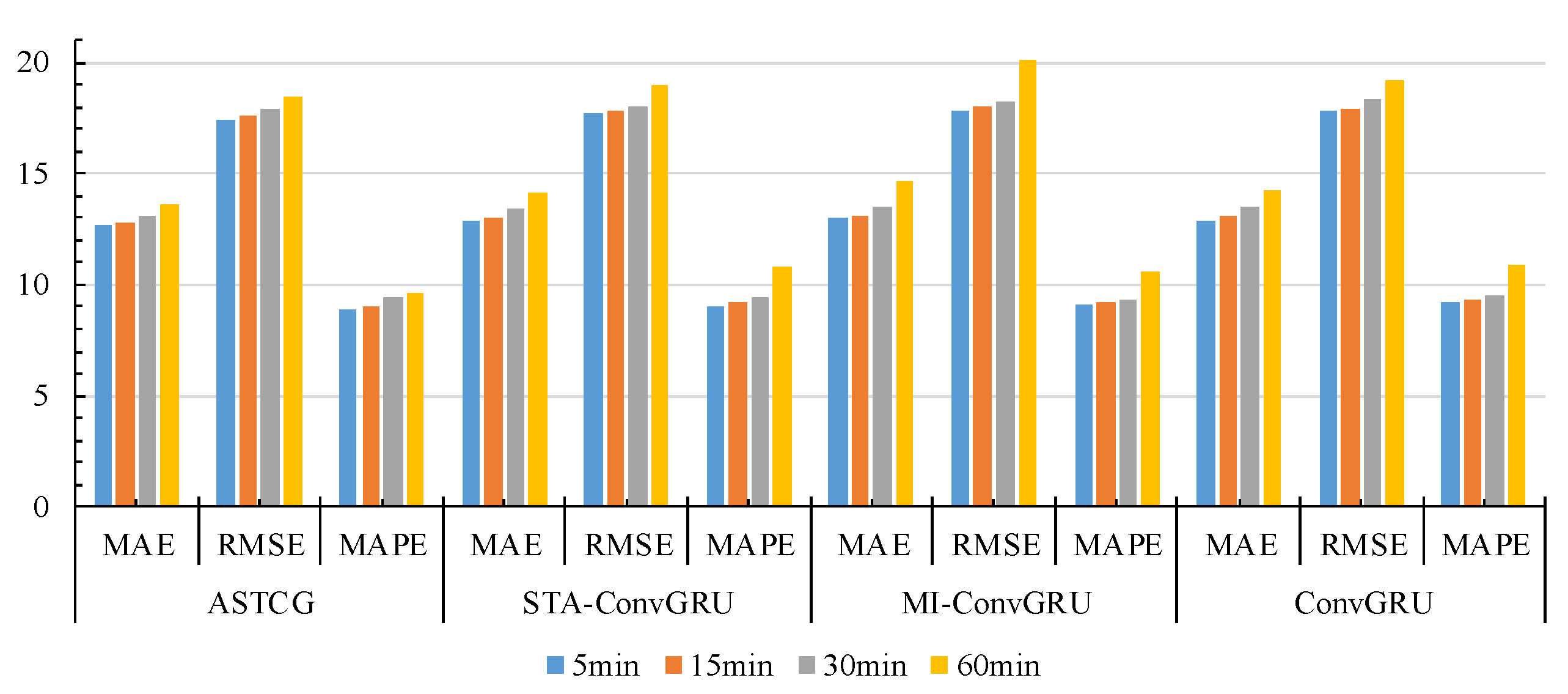
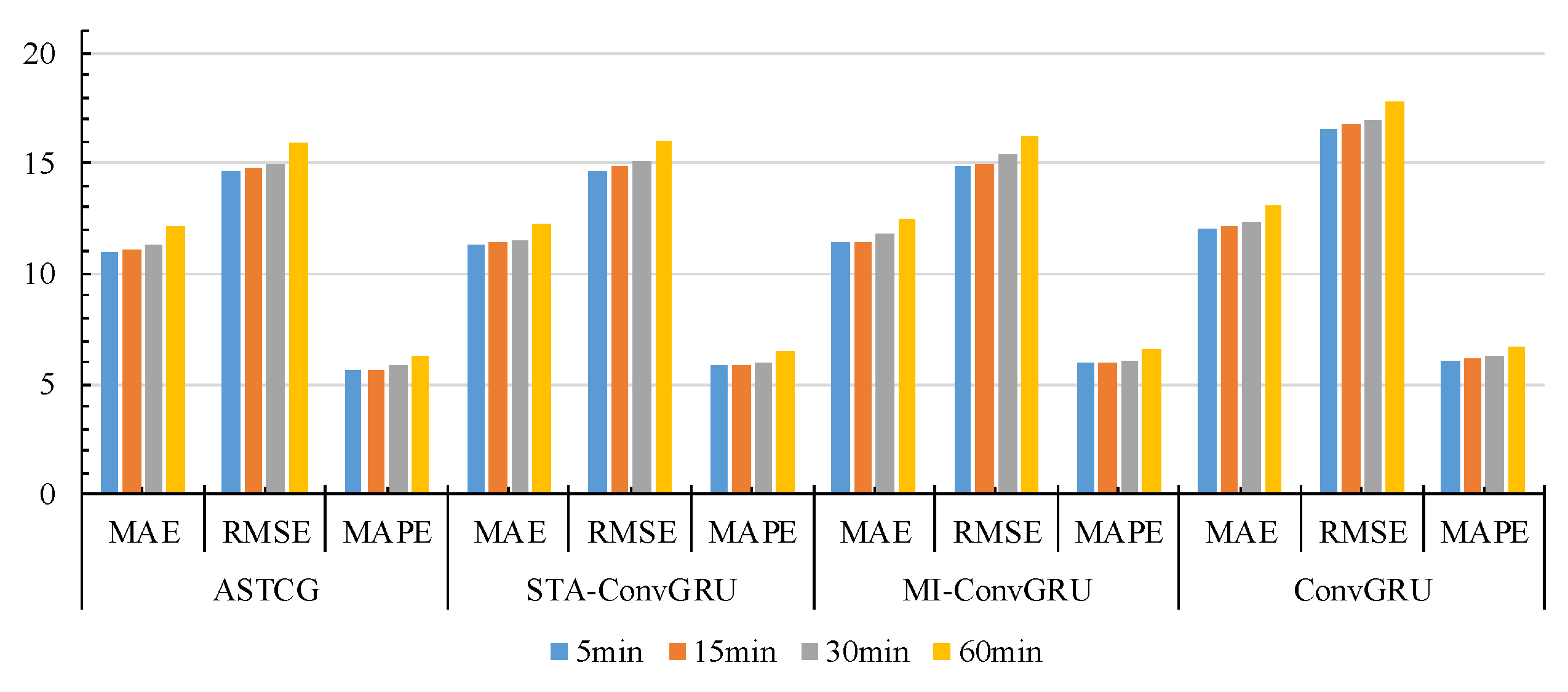
5.3. Ablation Experiments
- (a)
- ConvGRU: This model seamlessly combines a convolutional neural network with a recurrent neural network to capture the spatial–temporal dependencies of traffic flow data.
- (b)
- STA-ConvGRU: This model enhances ConvGRU by incorporating an attention module that quantifies the importance of historical time steps for improved prediction accuracy.
- (c)
- MI-ConvGRU: This model extends ConvGRU by incorporating a multi-input component for temporal data, which captures temporal dependence of traffic flow from multiple aspects by incorporating near-neighbor data, daily-periodic data, and weekly-periodic data as inputs.
6. Conclusions
Author Contributions
Funding
Institutional Review Board Statement
Data Availability Statement
Conflicts of Interest
References
- Zhang, J.; Wang, F.Y.; Wang, K.; Lin, W.H.; Xu, X.; Chen, C. Data-Driven Intelligent Transportation Systems: A Survey. IEEE Trans. Intell. Transp. Syst. 2011, 12, 1624–1639. [Google Scholar] [CrossRef]
- Yuan, J.; Fan, B. Synthesis of short-term traffic flow forecasting research progress. Urban Transp. China 2012, 10, 73–79. [Google Scholar]
- Ishak, S.; Al-Deek, H. Performance evaluation of short-term time-series traffic prediction model. J. Transp. Eng. 2002, 128, 490–498. [Google Scholar] [CrossRef]
- Dan, Y.; Zhang, Z.; Gan, P.; Ye, H.; Li, Q.; Deng, J. Performance Analysis of Corroded Grounding Devices with an Accurate Corrosion Model. CSEE J. Power Energy Syst. 2023, 9, 1235–1247. [Google Scholar]
- Liu, J.; Wei, G. A Summary of Traffic Flow Forecasting Methods. J. Highw. Transp. Res. Dev. 2004, 21, 82–85. [Google Scholar]
- Wang, H.; Liu, L.; Dong, S.; Qian, Z.; Wei, H. A novel work zone short-term vehicle-type specific traffic speed prediction model through the hybrid EMD–ARIMA framework. Transp. B Transp. Dyn. 2015, 4, 159–186. [Google Scholar] [CrossRef]
- Okutani, I.; Stephanedes, Y.J. Dynamic prediction of traffic volume through Kalman filtering theory. Transp. Res. Part B Methodol. 1984, 18, 1–11. [Google Scholar] [CrossRef]
- Hossain, M.Z.; Sohel, F.; Shiratuddin, M.F.; Laga, H. A Comprehensive Survey of Deep Learning for Image Captioning. ACM Comput. Surv. 2019, 51, 1–36. [Google Scholar] [CrossRef] [Green Version]
- Zhang, Z.; Yang, Y.; Zhao, H.; Xiao, R. Prediction method of line loss rate in low-voltage distribution network based on multi-dimensional information matrix and dimensional attention mechanism-long-and short-term time-series network. IET Gener. Transm. Distrib. 2022, 16, 4187–4203. [Google Scholar] [CrossRef]
- Dai, Z.; Yang, Z.; Yang, Y.; Carbonell, J.G.; Le, Q.; Salakhutdinov, R. Transformer-XL: Attentive Language Models beyond a Fixed-Length Context. arXiv 2019, arXiv:1901.02860. [Google Scholar]
- Hochreiter, S.; Schmidhuber, J. Long short-term memory. Neural Comput. 1997, 9, 1735–1780. [Google Scholar] [CrossRef]
- Chung, J.; Gulcehre, C.; Cho, K.; Bengio, Y. Empirical evaluation of gated recurrent neural networks on sequence modeling. arXiv 2014, arXiv:1412.3555. [Google Scholar]
- Guo, S.; Lin, Y.; Li, S.; Chen, Z.; Wan, H. Deep Spatial-Temporal 3D Convolutional Neural Networks for Traffic Data Forecasting. IEEE Trans. Intell. Transp. Syst. 2019, 20, 1–14. [Google Scholar] [CrossRef]
- Li, Y.; Yu, R.; Shahabi, C.; Liu, Y. Diffusion Convolutional Recurrent Neural Network: Data-Driven Traffic Forecasting. arXiv 2017, arXiv:1707.01926. [Google Scholar]
- Shi, X.; Chen, Z.; Wang, H.; Yeung, D.Y.; Wong, W.K.; Woo, W.C. Convolutional LSTM Network: A Machine Learning Approach for Precipitation Nowcasting; MIT Press: Cambridge, MA, USA, 2015; Volume 28, pp. 55–71. [Google Scholar]
- Liang, Y.; Ke, S.; Zhang, J.; Yi, X.; Yu, Z. GeoMAN: Multi-level Attention Networks for Geo-sensory Time Series Prediction. In Proceedings of the International Joint Conference on Artificial Intelligence, Stockholm, Sweden, 13–19 July 2018; Volume 2018, pp. 1–16. [Google Scholar]
- Guo, S.; Lin, Y.; Feng, N.; Song, C.; Wan, H. Attention Based Spatial-Temporal Graph Convolutional Networks for Traffic Flow Forecasting. In Proceedings of the AAAI Conference on Artificial Intelligence, Honolulu, HI, USA, 27 January–1 February 2019; Volume 33, pp. 922–929. [Google Scholar]
- Wang, Y.; Zheng, J.; Du, Y.; Huang, C.; Li, P. Traffic-GGNN: Predicting Traffic Flow via Attentional Spatial-Temporal Gated Graph Neural Networks. IEEE Trans. Intell. Transp. Syst. 2022, 23, 18423–18432. [Google Scholar] [CrossRef]
- Xiong, J.; Xiong, Z.; Zhuang, Y.; Cheong, J.W.; Dempster, A.G. Fault-Tolerant Cooperative Positioning Based on Hybrid Robust Gaussian Belief Propagation. IEEE Trans. Intell. Transp. Syst. 2023, 24, 6425–6431. [Google Scholar] [CrossRef]
- Fang, M.; Tang, L.; Yang, X.; Chen, Y.; Li, C.; Li, Q. FTPG: A Fine-Grained Traffic Prediction Method With Graph Attention Network Using Big Trace Data. IEEE Trans. Intell. Transp. Syst. 2022, 23, 5163–5175. [Google Scholar] [CrossRef]
- Jian, W.; Wei, D.; Guo, Y. New Bayesian combination method for short-term traffic flow forecasting. Transp. Res. Part C 2014, 43, 79–94. [Google Scholar]
- Shahriari, S.; Ghasri, M.; Sisson, S.A.; Rashidi, T. Ensemble of ARIMA: Combining Parametric and Bootstrapping Technique for Traffic Flow Prediction. Transp. A Transp. Sci. 2020, 16, 1552–1573. [Google Scholar] [CrossRef]
- Lint, H.V.; Hinsbergen, C.V. Short-Term Traffic and Travel Time Prediction Models. Transp. Res. E-Circ. 2012, 22, 22–41. [Google Scholar]
- Jeong, Y.S.; Byon, Y.J.; Castro-Neto, M.M.; Easa, S.M. Supervised Weighting-Online Learning Algorithm for Short-Term Traffic Flow Prediction. IEEE Trans. Intell. Transp. Syst. 2013, 14, 1700–1707. [Google Scholar] [CrossRef]
- Wang, Z.; Ji, S.; Yu, B. Short-Term Traffic Volume Forecasting with Asymmetric Loss Based on Enhanced KNN Method. Math. Probl. Eng. 2019, 2019, 1–11. [Google Scholar] [CrossRef] [Green Version]
- Luo, X.; Li, D.; Zhang, S. Traffic Flow Prediction during the Holidays Based on DFT and SVR. J. Sens. 2019, 2019, 1–10. [Google Scholar] [CrossRef] [Green Version]
- Castro-Neto, M.; Jeong, Y.S.; Jeong, M.K.; Han, L.D. Online-SVR for short-term traffic flow prediction under typical and atypical traffic conditions. Expert Syst. Appl. 2009, 36, 6164–6173. [Google Scholar] [CrossRef]
- Ma, X.; Tao, Z.; Wang, Y.; Yu, H.; Wang, Y. Long short-term memory neural network for traffic speed prediction using remote microwave sensor data. Transp. Res. Part C Emerg. Technol. 2015, 54, 187–197. [Google Scholar] [CrossRef]
- Wang, L.; Chai, D.; Liu, X.; Chen, L.; Chen, K. Exploring the Generalizability of Spatio-Temporal Traffic Prediction: Meta-Modeling and an Analytic Framework. IEEE Trans. Knowl. Data Eng. 2021, 4, 1–16. [Google Scholar] [CrossRef]
- Guo, S.; Lin, Y.; Wan, H.; Li, X.; Cong, G. Learning Dynamics and Heterogeneity of Spatial-Temporal Graph Data for Traffic Forecasting. IEEE Trans. Knowl. Data Eng. 2021, 5, 1–10. [Google Scholar] [CrossRef]
- Zhang, Q.; Yu, K.; Guo, Z. Graph Neural Network-Driven Traffic Forecasting for the Connected Internet of Vehicles. IEEE Trans. Netw. Sci. Eng. 2022, 4, 3015–3027. [Google Scholar] [CrossRef]
- Zhang, Q.; Liu, S. Urban traffic flow prediction model based on BP artificial neural network in Beijing area. J. Discret. Math. Sci. Cryptogr. 2018, 21, 849–858. [Google Scholar] [CrossRef]
- Yang, B.; Sun, S.; Li, J.; Lin, X.; Tian, Y. Traffic flow prediction using LSTM with feature enhancement. Neurocomputing 2019, 332, 320–327. [Google Scholar] [CrossRef]
- Ma, X.; Zhuang, D.; He, Z.; Ma, J.; Wang, Y. Learning Traffic as Images: A Deep Convolutional Neural Network for Large-Scale Transportation Network Speed Prediction. Sensors 2017, 17, 818–833. [Google Scholar] [CrossRef] [Green Version]
- Ke, R.; Li, W.; Cui, Z.; Wang, Y. Two-Stream Multi-Channel Convolutional Neural Network for Multi-Lane Traffic Speed Prediction Considering Traffic Volume Impact. Transp. Res. Rec. 2020, 2674, 459–470. [Google Scholar] [CrossRef]
- Zheng, H.; Lin, F.; Feng, X.; Chen, Y. A Hybrid Deep Learning Model With Attention-Based Conv-LSTM Networks for Short-Term Traffic Flow Prediction. IEEE Trans. Intell. Transp. Syst. 2020, 22, 1–11. [Google Scholar] [CrossRef]
- Zhai, L.; Yang, Y.; Song, S.; Ma, S.; Yang, F. Self-supervision Spatiotemporal Part-Whole Convolutional Neural Network for Traffic Prediction. Phys. A Stat. Mech. Its Appl. 2021, 579, 126141. [Google Scholar] [CrossRef]
- Gu, Z.; Chen, C.; Zheng, J.; Sun, L. Traffic flow prediction based on STG-CRNN. Control Decis. 2022, 37, 645–653. [Google Scholar]
- Zhao, L.; Song, Y.; Zhang, C.; Liu, Y.; Li, H. T-GCN: A Temporal Graph Convolutional Network for Traffic Prediction. IEEE Trans. Intell. Transp. Syst. 2019, 21, 1–11. [Google Scholar] [CrossRef] [Green Version]
- Zhang, Q.; Chang, J.; Meng, G.; Xiang, S.; Pan, C. Spatio-Temporal Graph Structure Learning for Traffic Forecasting. In Proceedings of the AAAI Conference on Artificial Intelligence, New York, NY, USA, 7–12 February 2020; Volume 34, pp. 1177–1185. [Google Scholar]
- Xu, M.; Liu, H. A flexible deep learning-aware framework for travel time prediction considering traffic event. Eng. Appl. Artif. Intell. 2021, 106, 104491–104505. [Google Scholar] [CrossRef]
- Wang, C.; Tian, R.; HU, J.; Ma, Z. A trend graph attention network for traffic prediction. Inf. Sci. 2023, 623, 275–292. [Google Scholar] [CrossRef]
- Zhang, T.; Guo, G. Graph Attention LSTM: A Spatio-Temperal Approach for Traffic Flow Forecasting. IEEE Intell. Transp. Syst. Mag. 2020, 14, 190–196. [Google Scholar] [CrossRef]
- Guo, K.; Hu, Y.; Qian, Z.; Sun, Y.; Yin, B. Dynamic Graph Convolution Network for Traffic Forecasting Based on Latent Network of Laplace Matrix Estimation. IEEE Trans. Intell. Transp. Syst. 2020, 23, 1–10. [Google Scholar] [CrossRef]
- Song, C.; Lin, Y.; Guo, S.; Wan, H. Spatial-temporal synchronous graph convolutional networks: A new framework for spatial-temporal network data forecasting. In Proceedings of the AAAI Conference on Artificial Intelligence, New York, NY, USA, 7–12 February 2020; Volume 34, pp. 914–921. [Google Scholar]
- Wei, C.; Sheng, J. Spatial-temporal graph attention networks for traffic flow forecasting. In Proceedings of the IOP Conference Series: Earth and Environmental Science; IOP: Bristol, UK, 2020; Volume 587, pp. 65–78. [Google Scholar]
- Shi, X.; Qi, H.; Shen, Y.; Wu, G.; Yin, B. A Spatial–Temporal Attention Approach for Traffic Prediction. IEEE Trans. Intell. Transp. Syst. 2021, 22, 4909–4918. [Google Scholar] [CrossRef]
- Yu, B.; Yin, H.; Zhu, Z. Spatio-temporal Graph Convolutional Neural Network: A Deep Learning Framework for Traffic Forecasting. Statistics 2017, 22, 1–13. [Google Scholar]


| Datasets | PEMS04 | PEMS08 |
|---|---|---|
| Goal node number | 104, 307 | 58, 100 |
| Number of node | 307 | 170 |
| Train time range | 1 January 2018–4 February 2018 | 1 July 2016–7 August 2016 |
| Validation time range | 5 February 2018–16 February 2018 | 8 August 2016–19 August 2016 |
| Test time range | 17 February 2018–28 February 2018 | 20 August 2016–31 August 2016 |
| Model | Node 307 of the PEMS04 | Node 104 of the PEMS04 | ||||
|---|---|---|---|---|---|---|
| MAE | RMSE | MAPE | MAE | RMSE | MAPE | |
| HA | 19.73 | 26.32 | 18.04% | 20.32 | 26.18 | 18.41% |
| BP | 18.64 | 25.07 | 13.39% | 19.14 | 25.73 | 15.23% |
| LSTM | 16.81 | 22.94 | 11.78% | 17.40 | 23.87 | 15.21% |
| GRU | 16.94 | 22.72 | 11.76% | 17.39 | 23.75 | 13.91% |
| STGCN | 16.24 | 22.07 | 11.41% | 14.94 | 20.43 | 12.02% |
| T-GCN | 16.36 | 21.96 | 11.34% | 16.48 | 22.45 | 12.50% |
| ASTCG | 14.71 | 19.90 | 10.84% | 14.58 | 19.80 | 11.20% |
| Model | Node 100 of the PEMS08 | Node 58 of the PEMS08 | ||||
|---|---|---|---|---|---|---|
| MAE | RMSE | MAPE | MAE | RMSE | MAPE | |
| HA | 16.7 | 21.45 | 8.45% | 16.21 | 21.32 | 9.12% |
| BP | 15.13 | 19.71 | 8.08% | 15.44 | 20.48 | 8.94% |
| LSTM | 14.26 | 18.66 | 7.37% | 15.14 | 20.10 | 8.77% |
| GRU | 14.95 | 19.62 | 7.44% | 15.12 | 20.11 | 8.81% |
| STGCN | 13.92 | 18.48 | 6.98% | 13.78 | 18.33 | 7.83% |
| T-GCN | 14.21 | 18.93 | 7.22% | 14.29 | 19.02 | 7.95% |
| ASTCG | 13.13 | 17.85 | 6.47% | 13.47 | 18.01 | 7.42% |
| Model | Horizon | Node 307 of the PEMS04 | Node 100 of the PEMS08 | ||||
|---|---|---|---|---|---|---|---|
| MAE | RMSE | MAPE | MAE | RMSE | MAPE | ||
| ConvGRU | 5 min | 12.89 | 17.81 | 9.23% | 12.02 | 16.57 | 6.09% |
| 15 min | 13.12 | 17.91 | 9.36% | 12.14 | 16.75 | 6.12% | |
| 30 min | 13.46 | 18.33 | 9.48% | 12.33 | 16.95 | 6.25% | |
| 60 min | 14.22 | 19.18 | 10.84% | 13.13 | 17.86 | 6.74% | |
| STA-ConvGRU | 5 min | 12.91 | 17.68 | 8.99% | 11.28 | 14.71 | 5.87% |
| 15 min | 12.97 | 17.78 | 9.21% | 11.42 | 14.92 | 5.89% | |
| 30 min | 13.36 | 18.02 | 9.43% | 11.55 | 15.12 | 5.98% | |
| 60 min | 14.11 | 19.01 | 10.8% | 12.28 | 16.01 | 6.43% | |
| MI-ConvGRU | 5 min | 12.98 | 17.77 | 9.09% | 11.38 | 14.86 | 5.92% |
| 15 min | 13.14 | 18.02 | 9.21% | 11.45 | 14.98 | 5.95% | |
| 30 min | 13.54 | 18.23 | 9.35% | 11.80 | 15.43 | 6.11% | |
| 60 min | 14.69 | 20.10 | 10.54% | 12.47 | 16.23 | 6.55% | |
| ASTCG | 5 min | 12.72 | 17.44 | 8.91% | 11.03 | 14.71 | 5.63% |
| 15 min | 12.82 | 17.58 | 9.04% | 11.09 | 14.75 | 5.68% | |
| 30 min | 13.12 | 17.91 | 9.46% | 11.31 | 14.98 | 5.85% | |
| 60 min | 13.59 | 18.47 | 9.66% | 12.13 | 15.89 | 6.25% | |
Disclaimer/Publisher’s Note: The statements, opinions and data contained in all publications are solely those of the individual author(s) and contributor(s) and not of MDPI and/or the editor(s). MDPI and/or the editor(s) disclaim responsibility for any injury to people or property resulting from any ideas, methods, instructions or products referred to in the content. |
© 2023 by the authors. Licensee MDPI, Basel, Switzerland. This article is an open access article distributed under the terms and conditions of the Creative Commons Attribution (CC BY) license (https://creativecommons.org/licenses/by/4.0/).
Share and Cite
Zhang, Q.; Chang, W.; Yin, C.; Xiao, P.; Li, K.; Tan, M. Attention-Based Spatial–Temporal Convolution Gated Recurrent Unit for Traffic Flow Forecasting. Entropy 2023, 25, 938. https://doi.org/10.3390/e25060938
Zhang Q, Chang W, Yin C, Xiao P, Li K, Tan M. Attention-Based Spatial–Temporal Convolution Gated Recurrent Unit for Traffic Flow Forecasting. Entropy. 2023; 25(6):938. https://doi.org/10.3390/e25060938
Chicago/Turabian StyleZhang, Qingyong, Wanfeng Chang, Conghui Yin, Peng Xiao, Kelei Li, and Meifang Tan. 2023. "Attention-Based Spatial–Temporal Convolution Gated Recurrent Unit for Traffic Flow Forecasting" Entropy 25, no. 6: 938. https://doi.org/10.3390/e25060938