
On the Uncertainty Properties of the Conditional Distribution of the Past Life Time


Abstract
:1. Introduction
2. The Past Life-Time Uncertainty in Coherent Systems
- (a)
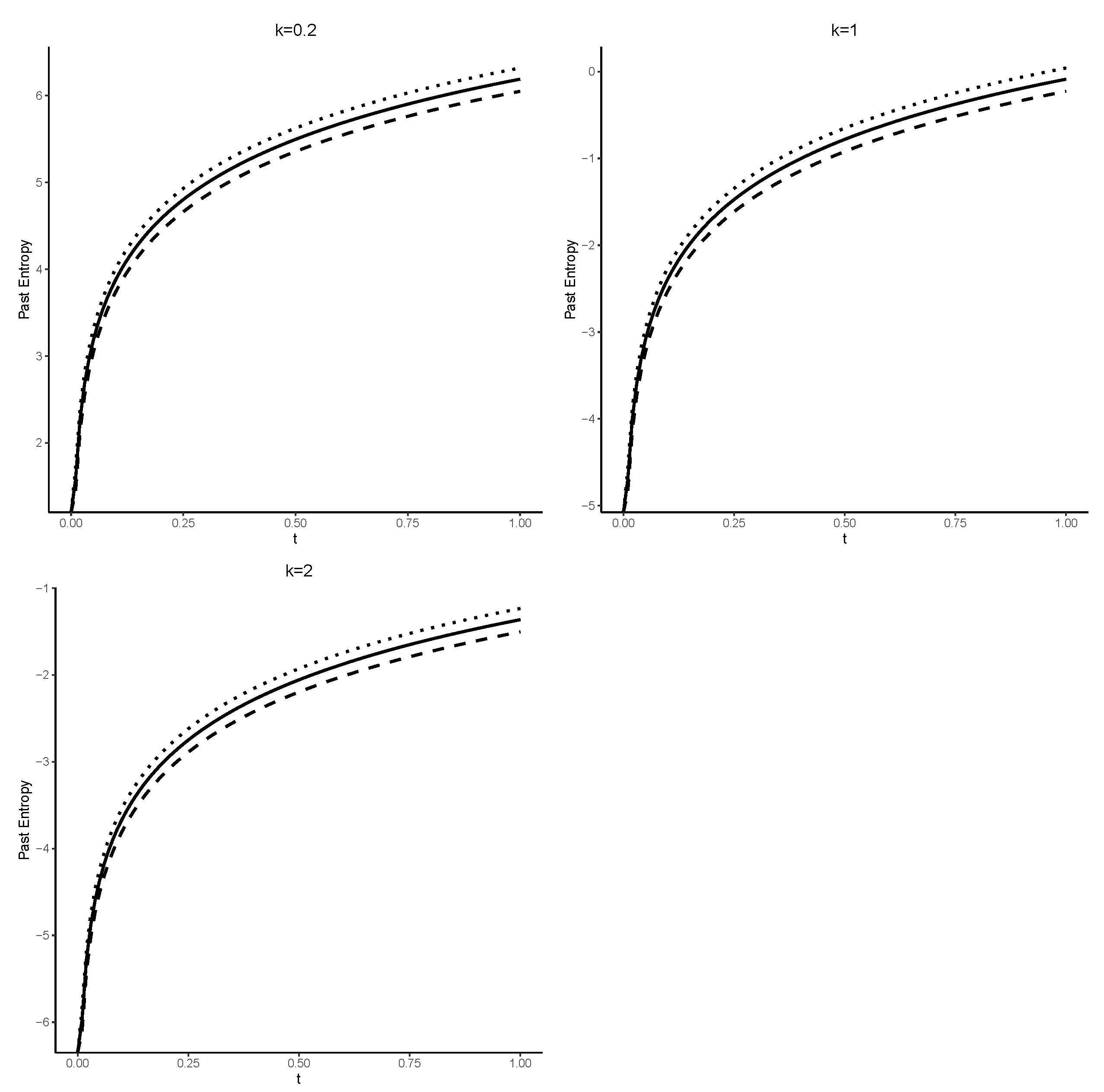
- It is seen that the entropy of is an increasing function of time We note that the uniform distribution has the DRHR property, and therefore, is an increasing function of time t, as we expected based on Theorem 1.
- (b)
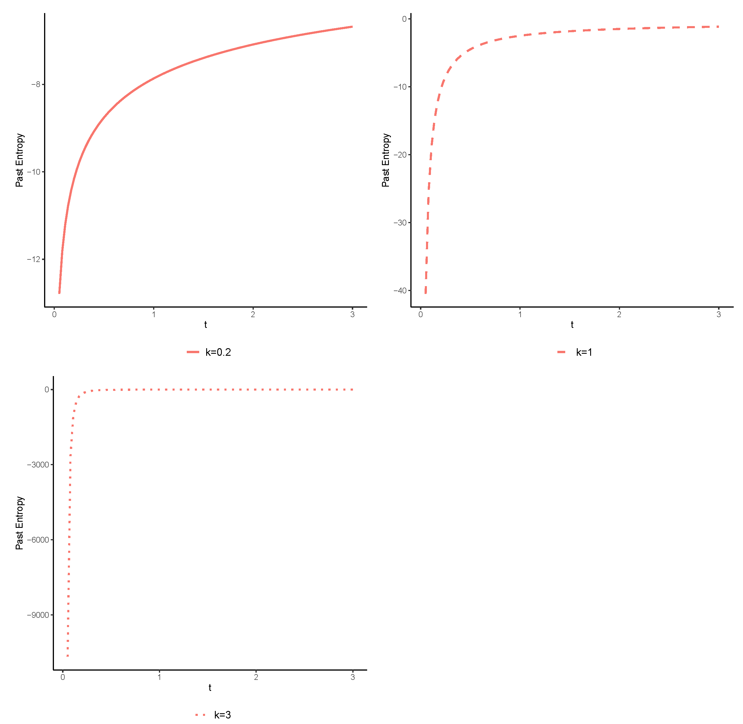
- Let us assume that X follows the cdfOne can see thatfor all Upon recalling (9), we obtainfor all For several choices of k, we have shown the exact value of with respect to time t in Figure 1. It is obvious that is an increasing function of time t for all since X is DRHR, as can follow from Theorem 1.
3. Bounds for the Past Entropy
- (i)
- if and increases in u for all then .
- (ii)
- if and decreases in u for all then .
- (i)
- if increases in u for all then .
- (ii)
- if decreases in u for all then .
4. Jensen–Shannon Divergence of System
5. Concluding Remarks
Author Contributions
Funding
Informed Consent Statement
Data Availability Statement
Acknowledgments
Conflicts of Interest
References
- Ebrahimi, N.; Pellerey, F. New partial ordering of survival functions based on the notion of uncertainty. J. Appl. Probab. 1995, 32, 202–211. [Google Scholar] [CrossRef]
- Shannon, C.E. A mathematical theory of communication. Bell Syst. Tech. J. 1948, 27, 379–423. [Google Scholar] [CrossRef] [Green Version]
- Ebrahimi, N. How to measure uncertainty in the residual life time distribution. Sankhyā Indian J. Stat. Ser. A 1996, 58, 48–56. [Google Scholar]
- Di Crescenzo, A.; Longobardi, M. Entropy-based measure of uncertainty in past lifetime distributions. J. Appl. Probab. 2002, 39, 434–440. [Google Scholar] [CrossRef]
- Nair, N.U.; Sunoj, S. Some aspects of reversed hazard rate and past entropy. Commun.-Stat.-Theory Methods 2021, 32, 2106–2116. [Google Scholar] [CrossRef]
- Shangari, D.; Chen, J. Partial monotonicity of entropy measures. Stat. Probab. Lett. 2012, 82, 1935–1940. [Google Scholar] [CrossRef]
- Loperfido, N. Kurtosis-based projection pursuit for outlier detection in financial time series. Eur. J. Financ. 2020, 26, 142–164. [Google Scholar] [CrossRef]
- Gupta, R.C.; Taneja, H.; Thapliyal, R. Stochastic comparisons of residual entropy of order statistics and some characterization results. J. Stat. Theory Appl. 2014, 13, 27–37. [Google Scholar] [CrossRef] [Green Version]
- Thapliyal, R.; Taneja, H. Order statistics based measure of past entropy. Math. J. Interdiscip. Sci. 2013, 1, 63–70. [Google Scholar] [CrossRef] [Green Version]
- Toomaj, A.; Chahkandi, M.; Balakrishnan, N. On the information properties of working used systems using dynamic signature. Appl. Stoch. Model. Bus. Ind. 2021, 37, 318–341. [Google Scholar] [CrossRef]
- Kayid, M.; Alshehri, M.A. Tsallis Entropy of a Used Reliability System at the System Level. Entropy 2023, 25, 550. [Google Scholar] [CrossRef] [PubMed]
- Mesfioui, M.; Kayid, M.; Shrahili, M. Renyi Entropy of the Residual Lifetime of a Reliability System at the System Level. Axioms 2023, 12, 320. [Google Scholar] [CrossRef]
- Samaniego, F.J. System Signatures and Their Applications in Engineering Reliability; Springer Science & Business Media: Berlin/Heidelberg, Germany, 2007; Volume 110. [Google Scholar]
- Khaledi, B.E.; Shaked, M. Ordering conditional lifetimes of coherent systems. J. Stat. Plan. Inference 2007, 137, 1173–1184. [Google Scholar] [CrossRef]
- Kochar, S.; Mukerjee, H.; Samaniego, F.J. The “signature” of a coherent system and its application to comparisons among systems. Nav. Res. Logist. 1999, 46, 507–523. [Google Scholar] [CrossRef]
- Hwang, J.; Lin, G. On a generalized moment problem. II. Proc. Am. Math. Soc. 1984, 91, 577–580. [Google Scholar] [CrossRef]
- Toomaj, A.; Doostparast, M. On the Kullback Leibler information for mixed systems. Int. J. Syst. Sci. 2016, 47, 2458–2465. [Google Scholar] [CrossRef]
- Asadi, M.; Ebrahimi, N.; Soofi, E.S.; Zohrevand, Y. Jensen–Shannon information of the coherent system lifetime. Reliab. Eng. Syst. Saf. 2016, 156, 244–255. [Google Scholar] [CrossRef]
- Abdolsaeed, T.; Doostparast, M. A note on signature-based expressions for the entropy of mixed r-out-of-n systems. Nav. Res. Logist. 2014, 61, 202–206. [Google Scholar]
- Murthy, D.; Jiang, R. Parametric study of sectional models involving two Weibull distributions. Reliab. Eng. Syst. Saf. 1997, 56, 151–159. [Google Scholar] [CrossRef]
- Jiang, R.; Zuo, M.; Li, H.X. Weibull and inverse Weibull mixture models allowing negative weights. Reliab. Eng. Syst. Saf. 1999, 66, 227–234. [Google Scholar] [CrossRef]
- Castet, J.F.; Saleh, J.H. Single versus mixture Weibull distributions for nonparametric satellite reliability. Reliab. Eng. Syst. Saf. 2010, 95, 295–300. [Google Scholar] [CrossRef]
- Qiu, G.; Wang, L.; Wang, X. On extropy properties of mixed systems. Probab. Eng. Inf. Sci. 2019, 33, 471–486. [Google Scholar] [CrossRef]
- Toomaj, A.; Di Crescenzo, A.; Doostparast, M. Some results on information properties of coherent systems. Appl. Stoch. Model. Bus. Ind. 2018, 34, 128–143. [Google Scholar] [CrossRef]
- Shaked, M.; Shanthikumar, J.G. Stochastic Orders; Springer Science & Business Media: Berlin/Heidelberg, Germany, 2007. [Google Scholar]


Disclaimer/Publisher’s Note: The statements, opinions and data contained in all publications are solely those of the individual author(s) and contributor(s) and not of MDPI and/or the editor(s). MDPI and/or the editor(s) disclaim responsibility for any injury to people or property resulting from any ideas, methods, instructions or products referred to in the content. |
© 2023 by the authors. Licensee MDPI, Basel, Switzerland. This article is an open access article distributed under the terms and conditions of the Creative Commons Attribution (CC BY) license (https://creativecommons.org/licenses/by/4.0/).
Share and Cite
Kayid, M.; Shrahili, M. On the Uncertainty Properties of the Conditional Distribution of the Past Life Time. Entropy 2023, 25, 895. https://doi.org/10.3390/e25060895
Kayid M, Shrahili M. On the Uncertainty Properties of the Conditional Distribution of the Past Life Time. Entropy. 2023; 25(6):895. https://doi.org/10.3390/e25060895
Chicago/Turabian StyleKayid, Mohamed, and Mansour Shrahili. 2023. "On the Uncertainty Properties of the Conditional Distribution of the Past Life Time" Entropy 25, no. 6: 895. https://doi.org/10.3390/e25060895