1. Introduction
For a long time, the basic contradiction in the development of civil aviation was that the supply capacity could hardly meet the fast-growing market demand, resulting in substantial fluctuations in flight punctuality and frequent flight delays. During the 13th Five-Year Plan period, the Civil Aviation Administration of China (CAAC) implemented the policy of controlling the total amount and adjusting the structure, the problem has been alleviated to a certain extent by artificially controlling the total number of flights [
1]. From 2020, the total number of flights dropped sharply, and flight punctuality improved due to COVID-19 [
2]. However, as the global epidemic situation slows down, the total number of flights will continue to rise, and flight delays in the post-epidemic era will continue to warrant attention [
3]. Many factors can lead to flight delays, the most common ones include air traffic control reasons, weather reasons, airline reasons, and passenger reasons [
4], and with the growth of flight volume, the proportion of irregular flights caused by weather is increasing, approaching 60% in 2021 [
5]. Therefore, it is necessary to study the influence of weather factors on flight delays and improve the performance of flight delay prediction under bad weather.
The current flight delay prediction problem can be divided into two main categories: classification prediction of delay levels and regression prediction of delay times. Compared with classification prediction models, regression models can predict specific delay times, providing more granular guidance for practical application in the relevant sectors. The trending nature of the regression model itself makes it more advantageous in problems that examine significant associations between independent and dependent variables and the strength of the effects of multiple different independent variables on a dependent variable, and the flight delay problem is the result of the interaction of delay times with multiple characteristic factors in the data.
In the traditional machine algorithm to build the regression model, Luo et al. first used the phase space reconstruction theory to find that there are chaotic characteristics in the time series composed of flight arrival delays and built the flight delay prediction model by the support vector machine method [
6]. Churchill et al. studied the delay spread of a single flight in multiple chain airports based on two machine learning models, logistic regression and decision tree. Through experimental comparison, the prediction error of the logistic regression model is lower [
7]. Ma et al. established a chaotic short-term prediction model based on an extreme learning machine for the chaotic characteristics of flight delay time series [
8]. Luo et al. first added the characteristics of the aviation information network to the airport data and used the SVR method to obtain a nonlinear regression prediction model [
9]. He et al. built a flight delay prediction model based on the support vector machine regression method and used the feature with the highest correlation with the flight delay time in the data set as a variable to predict the overall delay level [
10]. Feng et al. designed a web service based on the linear regression method to predict whether and how long a flight will be delayed [
11]. Wang et al. built a flight delay model based on random forest regression and decision tree regression using real data sets from large domestic airports, and the model fit reached 0.83, reducing the risk of overfitting the model [
12].
With the continuous development and progress of prediction algorithms and the successful application of deep learning methods in various fields, recurrent neural networks are especially widely used in regression problems with time series [
13,
14,
15,
16,
17,
18,
19,
20]. LSTM (Long Short-Term Memory) [
21] has a strong feature extraction ability for time series data, so the prediction accuracy is significantly higher than traditional machine learning methods. Khanmohammadi et al. first adopted the model prediction of ANN, and the results were due to the traditional backpropagation algorithm [
22]. Kim et al. construct sequences for flight data and, in a single airport, employ an RNN model to predict flight delays [
23]. Li et al. built a regression prediction model based on the LSTM network by considering the correlation between the airline and airport in the time dimension and the space dimension which can fully extract the information of the flight data [
24]. Fu et al. proposed a data augmentation method for the unbalanced characteristics of the flight delay data set which improved the prediction performance of the model to a certain extent [
25]. Song et al. specifically constructed a neural network model for the flight segment from Shanghai Hongqiao Airport to Beijing Capital Airport to achieve dynamic prediction of flight arrival delays [
26]. Wang et al. positioned their research on the departure delay time prediction of a single flight and dynamically updated the training data through the latest flight operation data to build a flight delay prediction model [
27]. Zhang et al. collected the ADS-B signal as a dataset and extracted the spatial information in it and built a flight delay prediction model through the LSTM algorithm [
28]. Chen et al. used the Conv-LSTM algorithm to extract both temporal and spatial features and verified the effectiveness of the model on an urban rail transit dataset [
29]. Zhang et al. captured dynamic spatial dependencies through the PageRank algorithm, then input LSTM to weight the spatial dependencies, and finally added a temporal attention mechanism and introduced auxiliary features to improve the accuracy of the prediction model [
30].
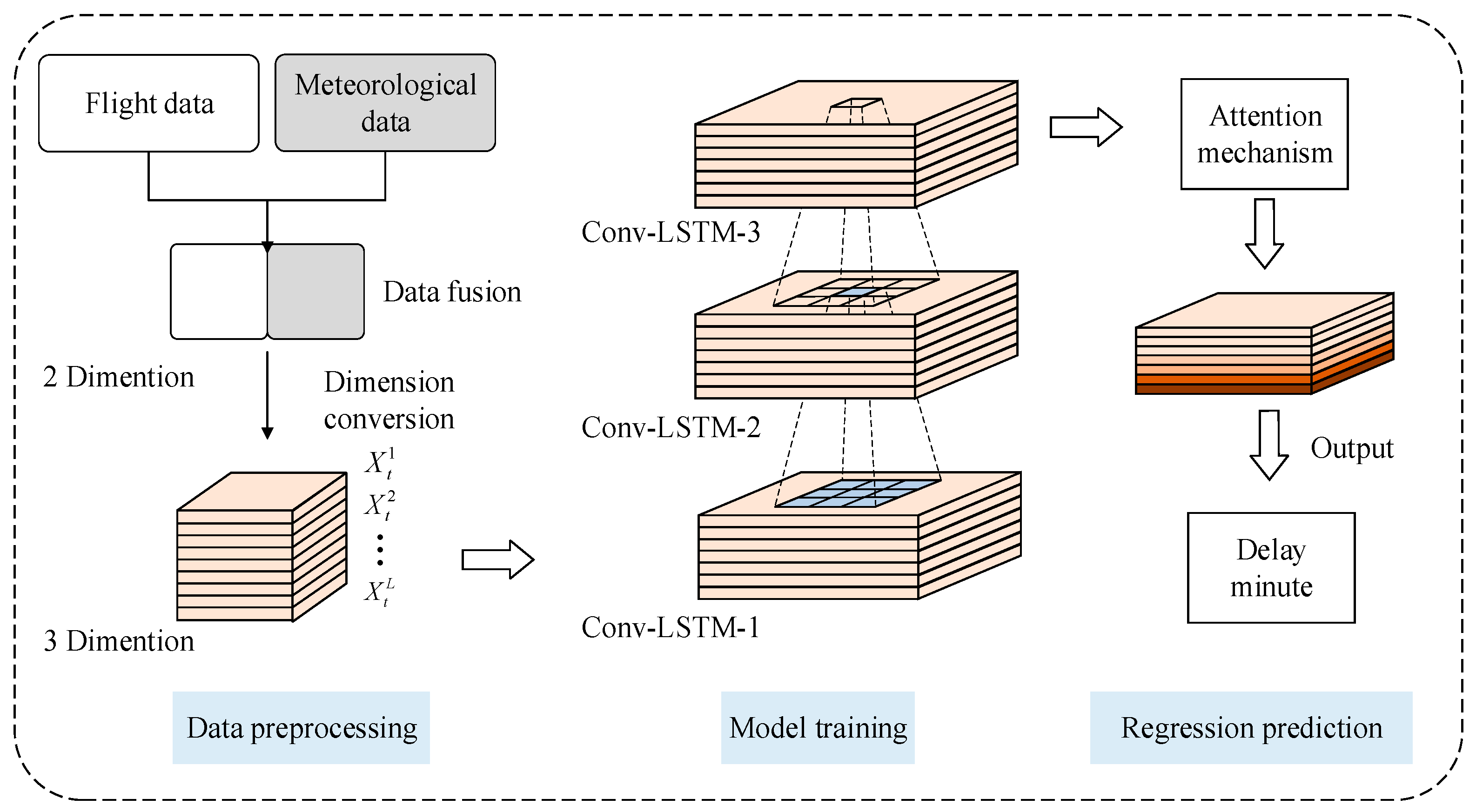
In the problem of flight delay regression prediction, a large number of scholars have studied the time dimension, but there are fewer flight delay prediction models that incorporate a comprehensive consideration of the spatial dimension. Aiming at the above problems, a flight delay prediction model based on Att-Conv-LSTM is proposed. On the basis of the time series in the extracted data, the meteorological data is added to expand the feature column, and the spatial information of the data is synchronously extracted by a convolution operation. It makes full use of the hidden spatial features within the samples and the temporal features between samples and then adds the attention mechanism module to improve the learning efficiency of the algorithm. In this paper, the validity of the proposed model is verified against the flight data of four domestic airports, and the influence of different factors, such as meteorological data and sequence length on the delay state, as well as the weight distribution of the attention module in the time series network are discussed.
3. Conv-LSTM Network Based on Attention Mechanism
The attention mechanism was first applied to computer vision. In 2014, the Google team [
33] added the attention mechanism to the deep learning recurrent neural network and achieved remarkable results in the problem of image classification. Then, the attention mechanism began to be widely used by scholars. Bahdanau et al. [
34] applied it to the field of natural language processing and also obtained good results in translation algorithms. In 2017, the Google team proposed the Transformer encoder–decoder algorithm [
35] which completely adopted the self-attention mechanism, abandoned the recurrent and convolutional neural networks commonly used in deep learning, and fully tapped the basic depth. The characteristics of neural networks are outstanding in many natural language processing tasks.
3.1. Network Description
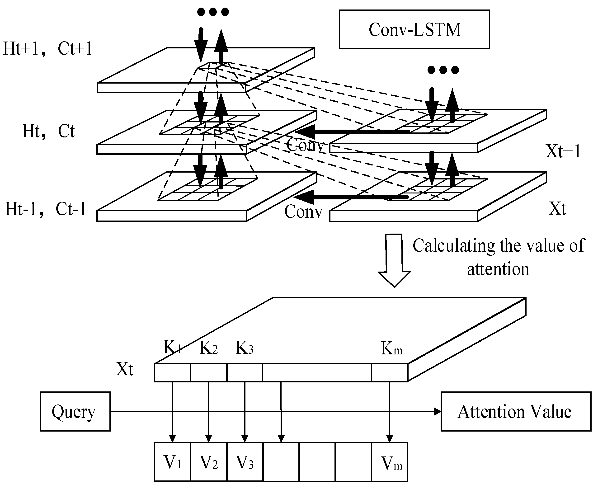
The essence of the attention mechanism stems from visual attention: when the visual system is facing a scene, it does not browse all the things in the scene but only looks at the places it focuses on. That is to say when the algorithm learns that in a scene, a certain part of the information is always highly related to the label; the next time it learns in a similar scene, the algorithm will focus on this information and try not to look at other sections for efficiency. The attention-based Conv-LSTM network structure is shown in
Figure 5.
In the network structure, Query (hereinafter referred to as Q) is an element in a given target, and (hereinafter referred to as K) is a part of the key value that constitutes the element. That is, the Keywords: By calculating the relationship between Q and each K, you can get each weight coefficient of the corresponding value of K and then the weighted summation, the final attention weight value is obtained. The calculation steps can generally be divided into the following three steps: (1) Calculate the similarity between Q and K to obtain the weight; (2) Normalize the calculated weight; (3) With the normalized weights and weighted sum, the result of the weighted sum is the final attention value. However, since attention is not an independent model, it just adds new information, and its variant does not propose a new definition of network layer, so it can only be called an attention mechanism module not a new model.
The core part of the attention is a series of weight parameters. It iteratively learns the degree of association between each element and the label in the sequence and then reassigns the original input according to its correlation. The weight parameter is assigned by the attention module. The introduction of the attention mechanism module will assign different attention sizes to different vectors in a sequence, reflecting the influence of each vector on predicting the current information. Due to the introduction of new information, the efficiency of network learning will be greatly improved.
3.2. Feature Extraction
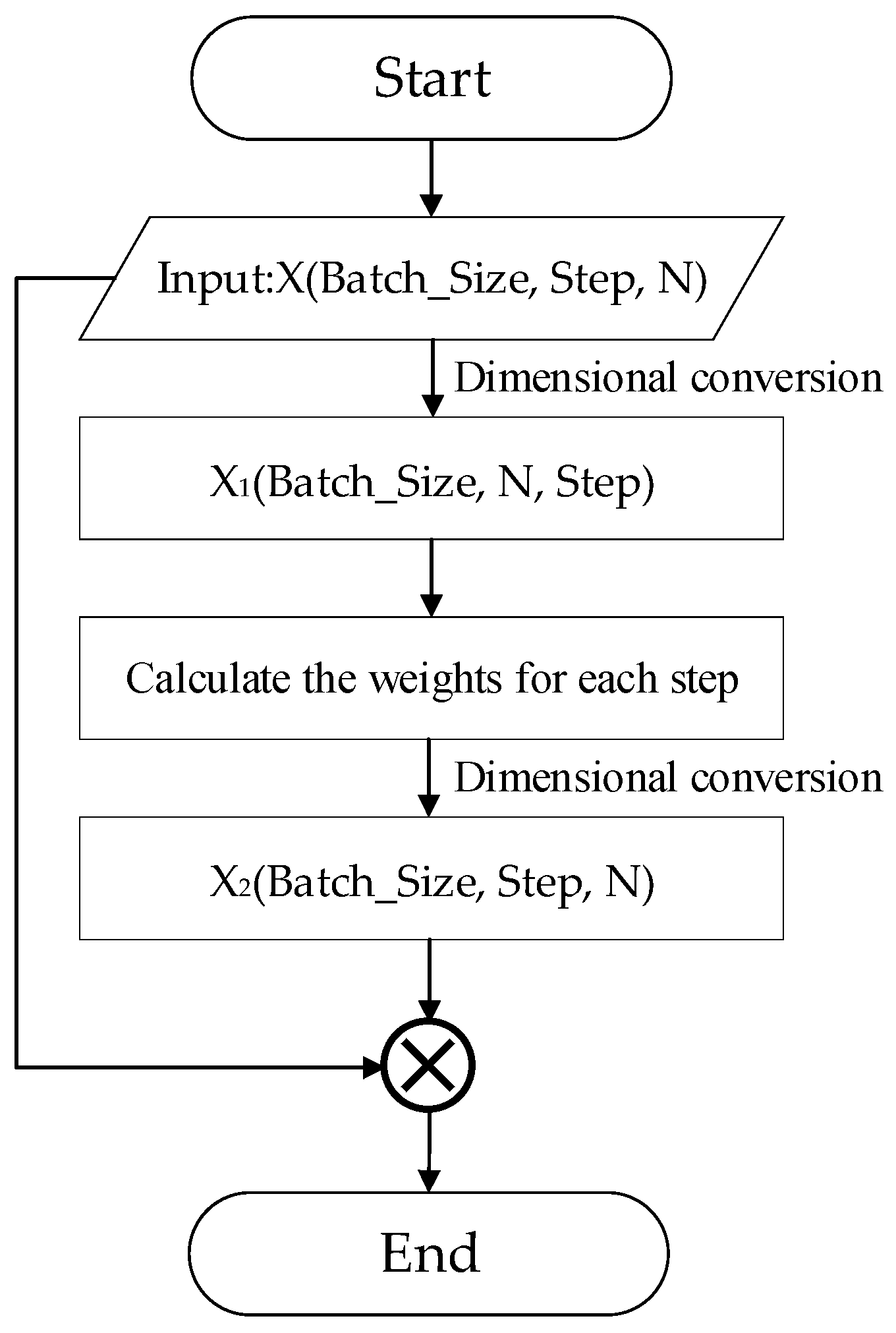
The essence of the attention mechanism is to perform a series of weighted sum operations on the input by generating a weight coefficient for a specific label to identify the importance of the features in the input to the target. The following mainly introduces the basic principles of the attention mechanism to further understand the details of feature extraction inside the regression model. Its implementation is shown in
Figure 6:
After the output of the Conv-LSTM network, we can obtain an output X with dimension (Batch_Size, Step, N), where Batch_Size is the size of the batch, Step denotes the length of the sequence, and N is the number of network cells. Firstly, X is treated as the feature of each time node as the input in
Figure 6 which is transformed into X
1 (Batch_Size, N, Step) after dimensional conversion to flip the second and third dimensions. Then, the weights of each feature in each step are calculated using the fully connected layer and Softmax classifier, and then the second and third dimensions are reduced after dimensional conversion to obtain X
2 (Batch_Size, Step, N). Finally, X
2 is multiplied with the input, that is, the weights of each step, multiplied by their features to obtain the final output value of the attention mechanism.
In order to realize the attention mechanism, we regard the input raw data as the form of <Key, Value> key-value pairs, and calculate the similarity coefficient between the keyword and the value according to the Query value in the given task target, and the corresponding value can be obtained. Then, use the weight coefficient to weight and sum the values to get the output. We use Q, K, and V to denote Query, Key, and Value, respectively. The formula for the attention weight coefficient
is as follows:
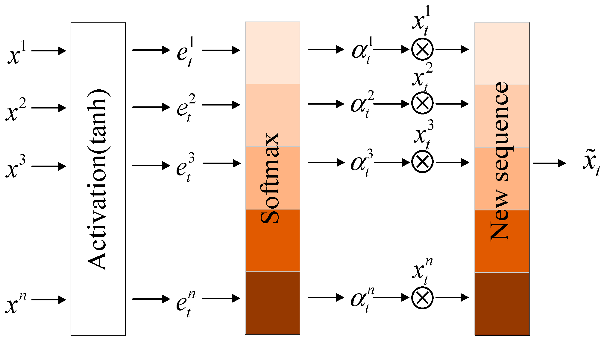
Figure 7 shows the input and output principles of the attention mechanism:
Taking a sample
with a sequence length of
as an example, as shown in
Figure 7, after the output of the Conv-LSTM network, the attention mechanism module connected to it first assigns the sequence an
activation function to obtain the sequence
, where
represents the intermediate state,
represents the hidden state, and
helps to find the optimal value during the iterative process. Then, through the
classifier, each vector in the sequence is assigned a weight value to obtain the weight sequence
. Finally, the weight sequence is transposed and summed with the original input sequence to obtain the final output of the attention module. The calculation formula of the whole process is as follows:
3.3. Model Training and Optimization
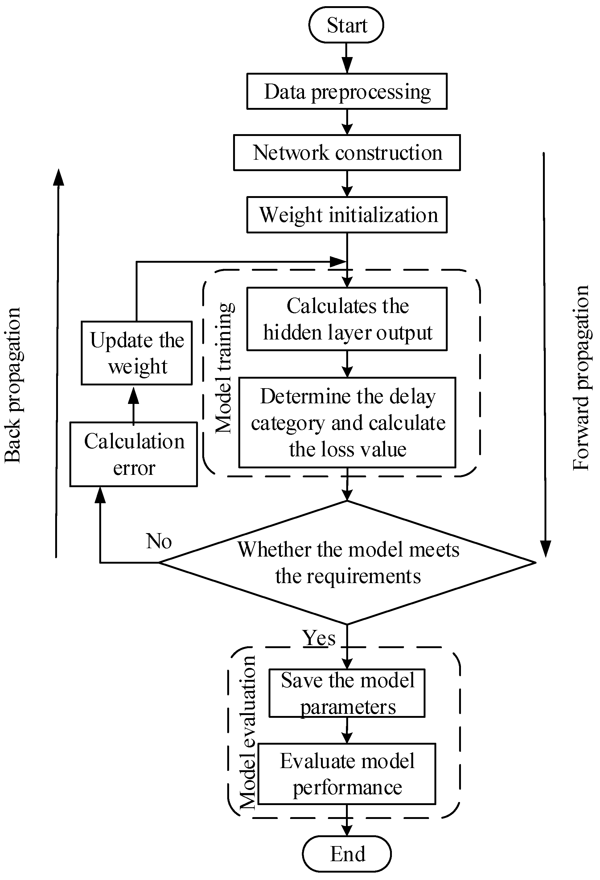
The training iteration based on the Att-Conv-LSTM prediction model consists of forward propagation and back propagation which, respectively, completes the forward propagation from the shallow layer to the deep layer and the reverse back propagation for continuous error correction. The overall training process of the model is shown in
Figure 8.
3.3.1. Model Training
The training of the model consists of two parts, forward propagation and back propagation. In forward propagation, this paper defines the initial weight value, activation function, and error function. After forward propagation, the calculation result and the error value are obtained. In back propagation, the error of the output layer is input to the hidden layer through back propagation, the hidden layer adjusts the weight value, and performs forward propagation again, thereby performing an iterative process of network training.
In this paper, the BP [
36] chain rule is used in the network training process to calculate the error term of the hidden layer, and then the weight gradient is calculated according to the error term. Formula (6) represents the derivation process for the weight matrix according to the full differentiation rule
, where
denotes the state of the neuron at layer
and
denotes the output of the neuron at layer
in matrix form. Then, calculate
according to the chain derivative rule, and write
as
for convenience of representation. The momentum factor is updated according to the results of the weight derivation as shown in Formula (7), and finally, the weight matrix is updated by Formula (8) for the next iterative process. The calculation formula of the weight gradient is as follows.
In the above formula, is the number of iterations, is the momentum factor which indicates the influence of the correction range of the previous weight on the current weight value, is the momentum variable, and is the learning rate which determines the speed of model training; is the weight decay coefficient.
In addition, deep learning generally divides the data set into training set and validation set. Each round of training will output the average loss value of the entire dataset through the above-mentioned forward propagation, and whether the loss value of training and validation is reduced synchronously as the standard, then continuously adjust the parameters in the network model through back propagation, and finally, obtain a set of parameters suitable for the network structure.
3.3.2. Model Optimization
In this paper, the Adam [
37] algorithm is used to optimize the network. This method is an improved first-order optimization algorithm based on the traditional stochastic gradient descent method which can dynamically change the weight value of the neural network during the iterative training of the neural network. The advantages of the Adam algorithm are: (1) The implementation method is simple, and there is no need to adjust hyperparameters. (2) It has an initial learning rate and can be adjusted automatically. (3) It is suitable for large sample size data and requires less memory. The detailed process of applying the Adam algorithm to gradient descent during neural network training is as follows: (1) Update the current number of iterations; as shown in Formula (9),
is the number of steps to update. (2) Calculate the gradient value of the network objective function to the parameters; as shown in Formula (10),
is the parameter to be updated,
is the loss function,
is the gradient obtained by the derivation of the objective function
to
. (3) Calculate the first-order matrix of the gradient values; as shown in Formula (11),
is the first-order moment decay coefficient,
is the first moment of the gradient
. (4) Calculate the second-order matrix of the gradient; as shown in Formula (12),
is the second-order moment Attenuation coefficient,
is the second moment of the gradient
. (5) Correct the first-order matrix; as shown in Formula (13),
is the bias correction of
. (6) Correct the second-order matrix; as shown in Formula (14),
is the bias correction of
. (7) Update the parameter
[
38].
4. Results
This section will introduce the experimental environment and basic parameters and compare and verify the model performance of the algorithm through various indicators. The regression prediction model based on Att-Conv-LSTM is an improved model based on the Conv-LSTM algorithm. Therefore, it is necessary to compare the network performance of the two from various indicators, such as error, and analyze the influence of flight information, weather factors, and sequence length on flight delays. The effect of prediction is verified, and the effectiveness of attention is verified by comparing the experimental results of different prediction models.
4.1. Experimental Environment and Parameter Configuration
The experimental environment processor is Intel Xeon E5Mu1620, the GPU memory is 11.92GiB, the operating system is Ubuntu16.04 (64-bit), the experimental platform is the Tensorflow 1.10.0 deep learning framework developed by Facebook, and the development language is a python language using Pycharm as python development tool to facilitate better debugging and management of the program.
The experimental data uses domestic flight data from 2019 to 2020. The experiment in this chapter uses the total flight data set. The data set contains 72 flight and meteorological features. The features finally input into the neural network are a three-dimensional matrix.
The structure of the flight delay prediction model based on Att-Conv-LSTM is designed according to
Figure 1. The network with different layers in the feature extraction part has the same structure except for the number of filters in the dense block. In this experiment, a random seed is set for the current GPU to ensure consistent training results each time. The experimental hyperparameters mainly include the selection of loss function and optimizer, the setting of learning rate correlation value, etc. The complete hyperparameter configuration of the experiment is shown in
Table 2.
4.2. Influence of Meteorological Data on Model Performance
This subsection discusses the improvement in model performance brought about by meteorological data in regression models.
Table 3 lists the comparison of prediction errors based on the Conv-LSTM network, Beijing Capital Airport fused, and unfused meteorological data.
According to the data in the table, it can be seen that in the regression model, the integration of meteorological data with 1 min precision did not bring about an increase in the sample size, but rather a decrease due to data pre-processing that removed rows with a small number of null values in the meteorological data features. The error after incorporation was reduced by 7.21.
4.3. The Effect of Sequence Length on Model Performance
In the regression model, the network used in this paper is more effective for information extraction in the time dimension. Since the sequence length is an important parameter in the recurrent neural network series, this section will discuss the impact of the sequence length on the network results during the serialization process. In this paper, five different step size parameters are tested, and the data set used is the flight and meteorological data of Beijing Capital Airport. The final accuracy is shown in
Table 4.
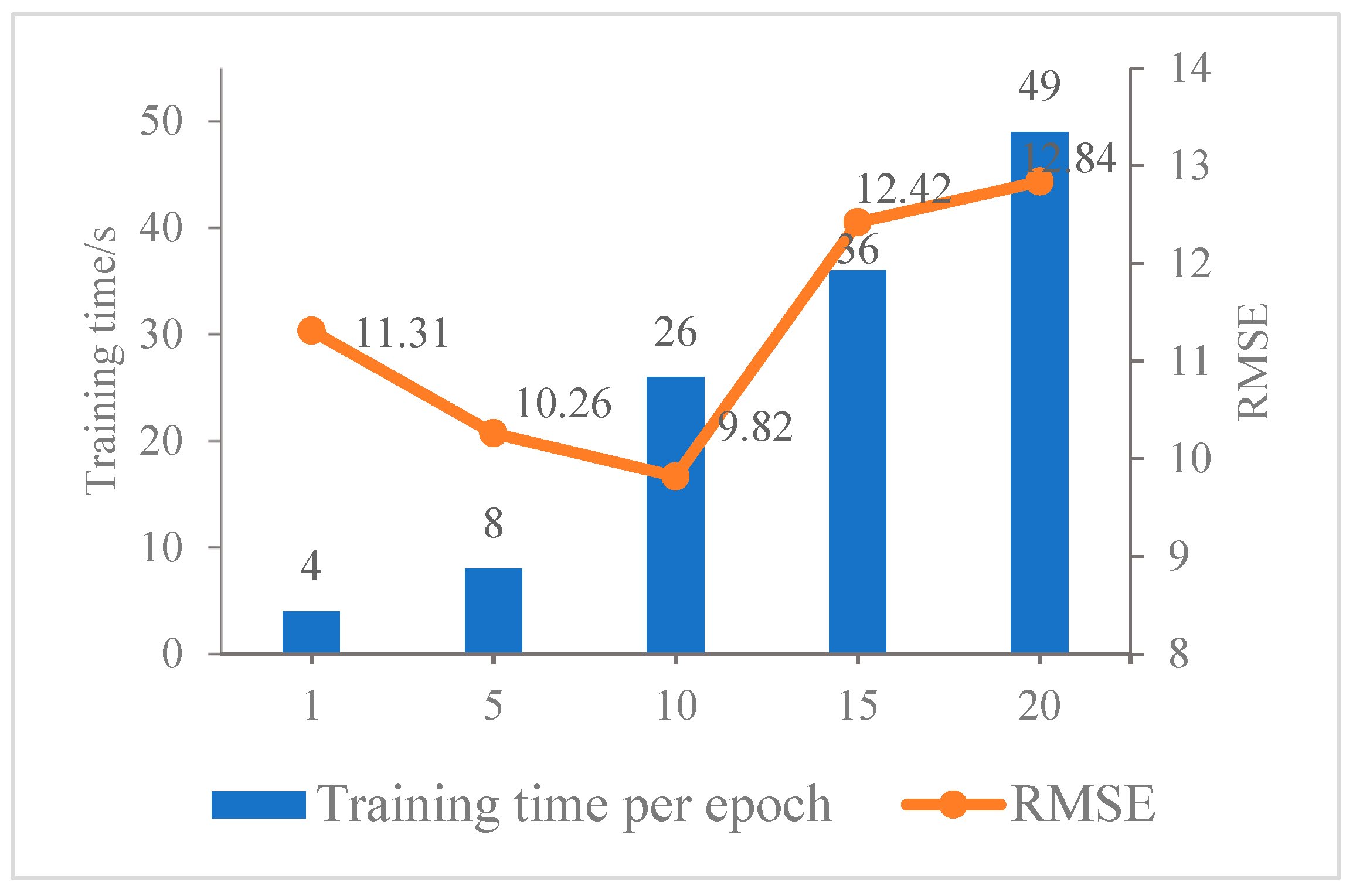
Table 4 lists the change of the accuracy with the increase in sequence length. The comparison shows that when the sequence length is 10, the RMSE reaches the lowest value of 9.82.
Figure 9 shows a graph of the model error RMSE versus training time as the sequence length increases. It can be seen from the figure that with the increase in the sequence length, the error of the model shows a downward trend. When the sequence length reaches 10, the error value is the lowest, but it is not that the longer the sequence length, the model performs better. As sequence length increases, the data contains more information, and the prediction results may be more accurate. However, the larger the sequence length is, the more difficult it is to capture the change of flight status in the short term, because there is a short-term temporal correlation between the states of flights, and flight states with too long a time gap have very little or no effect on the state of flights at the current time. It also causes the network to learn irrelevant information which causes data redundancy and increases the prediction error. When it is greater than 10, the model prediction error begins to decrease, indicating that flight delays only exist in a certain length of time series. At the same time, as the sequence length increases, the training time also increases gradually.
The influence of the flight status after a long time on whether the flight at the current moment is delayed has been small or even disappeared. Therefore, the network will learn irrelevant information, resulting in data redundancy and increased errors. In addition, longer time series will consume more training time. Therefore, it is necessary to experiment to choose the appropriate sequence length so that the prediction error is within a small range. From the comparison of several sets of data in the chart, it can be seen that, in the regression model, 10 is a more appropriate time series length value. Therefore, in this paper, the value of the sequence length is 10 as the basic parameter of the subsequent experiments.
4.4. Comparative Analysis with Traditional Flight Delay Prediction Methods
In order to verify that the Att-Conv-LSTM method based on deep learning has greater advantages over traditional algorithms in terms of data processing as well as prediction accuracy, the results of different flight delay prediction models are compared separately as shown in
Table 5. Several regression models, Linear Regression [
11], Decision Tree Regression [
12], and Random Forest Regression [
12], are trained on the Shijiazhuang Zhengding Airport dataset which is described in detail in
Section 2.1.1. Among the above methods, Linear Regression constructs linear functions for input and output values, and Decision Tree Regression and Random Forest Regression are two classical traditional machine learning regression methods. With the same data set, Linear Regression has the largest error RMSE value, while Att-Conv-LSTM has the smallest error RMSE value. The effectiveness of the Att-Conv-LSTM method is verified by comparing it with several regression analysis methods.
4.5. Comparative Analysis with Different Time-Series Neural Network Flight Delay Prediction Methods
In this section, the experiment mainly compares the training errors of three different network models from the size of the loss value and discusses the role of model improvement in the iteration of the neural network algorithm.
The loss function is used to estimate the degree of inconsistency between the predicted value
of the model and the real value
. It is a non-negative real-valued function, usually represented by
. In general, the smaller the loss function, the better the robustness of the model and the better the performance.
Table 6 shows the loss values of the Bi-LSTM network, Conv-LSTM network, and Att-Conv-LSTM network model training.
It can be seen from the experimental results in
Table 6. Compared with Bi-LSTM, the Conv-LSTM network adds the convolution part, and the error is reduced by an average of 11.41% in the datasets of the four airports; compared with Conv-LSTM, Att-Conv-LSTM network adds an attention mechanism to further extract the time information in the data, and the error is reduced by an average of 10.83%.
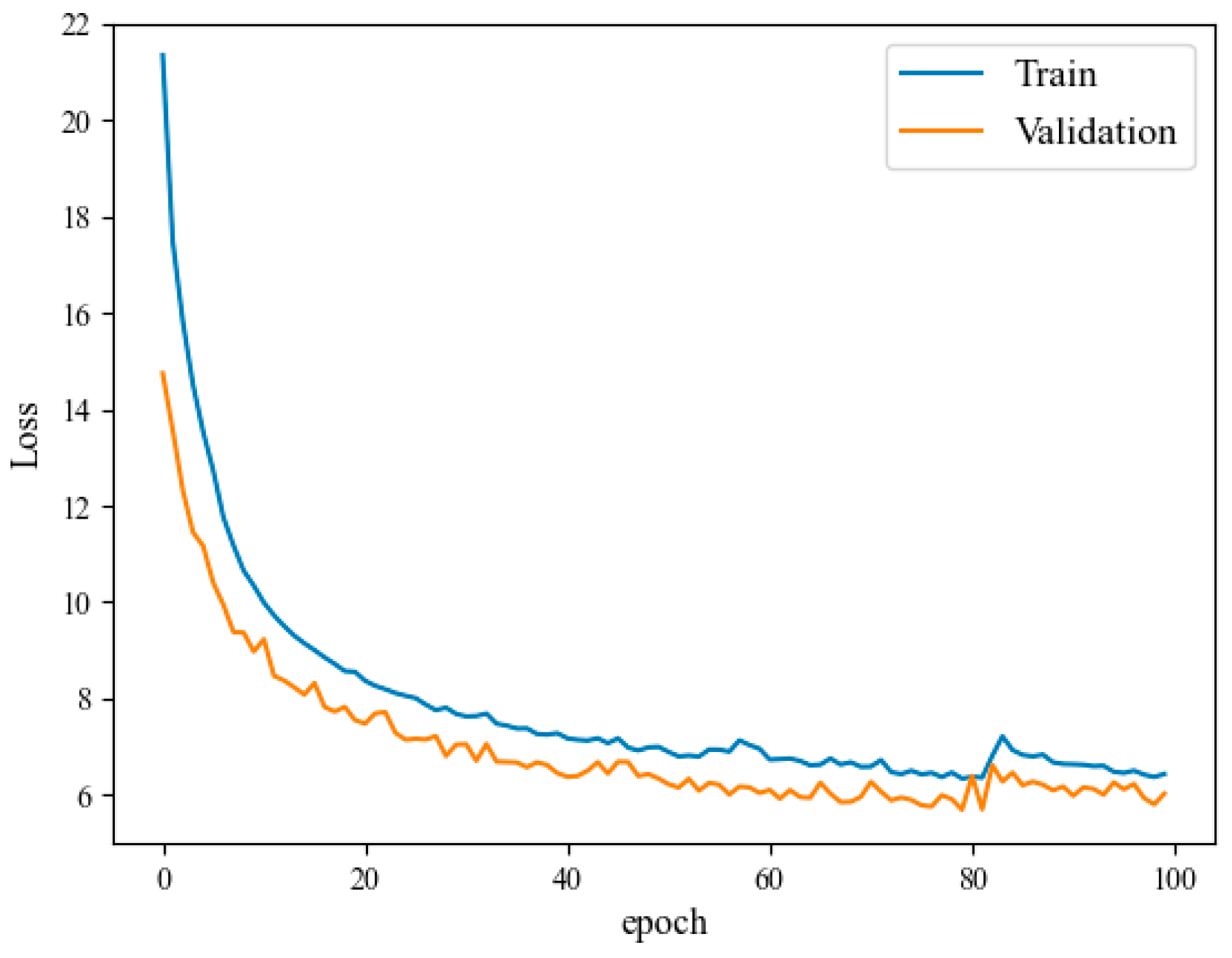
Figure 10 shows the decreasing trend of the training loss value based on the Att-Conv-LSTM network under the Shijiazhuang Airport dataset. The horizontal axis represents the number of training rounds, and the vertical axis represents the loss value. The sample size of the training set accounts for 80%, the sample size of the validation set accounts for 20%, and the number of model training rounds is 100 rounds. The sequence length of this experiment is 10, and the other hyperparameter configurations remain the same as in
Table 2.
The curves of the training set and the validation set of the four airports in this paper all fit well. Generally, the smaller the loss value, the better the training effect. As can be seen from the above figure, under the Att-Conv-LSTM network model, the loss values of the training set and the validation set decrease gently, and the fitting is good which is in line with the declining law of the general deep learning model of which the RMSE of the validation set is the lowest, reaching 6.81.
4.6. Feature Dimension Analysis of Attention Mechanism
In the classification model and regression model, the time dimension is the most important information in the network feature extraction, and the time series length is also an important parameter in the model. The attention mechanism added in the improved model can assign a weight to each step size in each sample. This section visualizes the weight parameters in the two models in order to see more intuitively the effect size of the time series in the network.
In the experimental analysis in
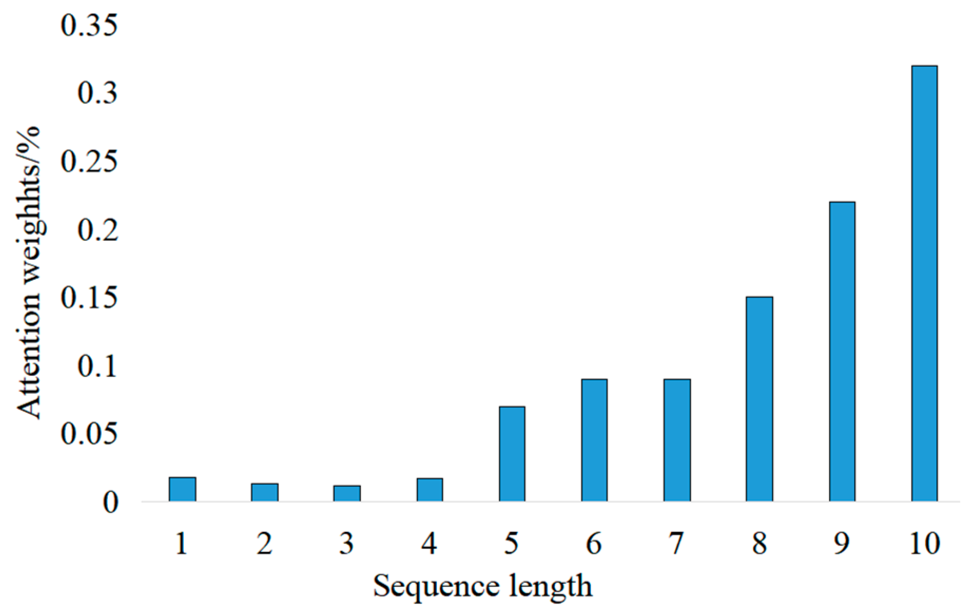
Section 4.3, the sequence length value of 10 is the most suitable choice for the regression model. Similarly, the weight of the attention feature is visualized as shown in
Figure 11. It can be seen that the closer to the forecast data to be predicted, the more weighted the bar data vector is in a sample with a stride of 10.


