
Improving the Process of Early-Warning Detection and Identifying the Most Affected Markets: Evidence from Subprime Mortgage Crisis and COVID-19 Outbreak—Application to American Stock Markets

Abstract
:1. Introduction
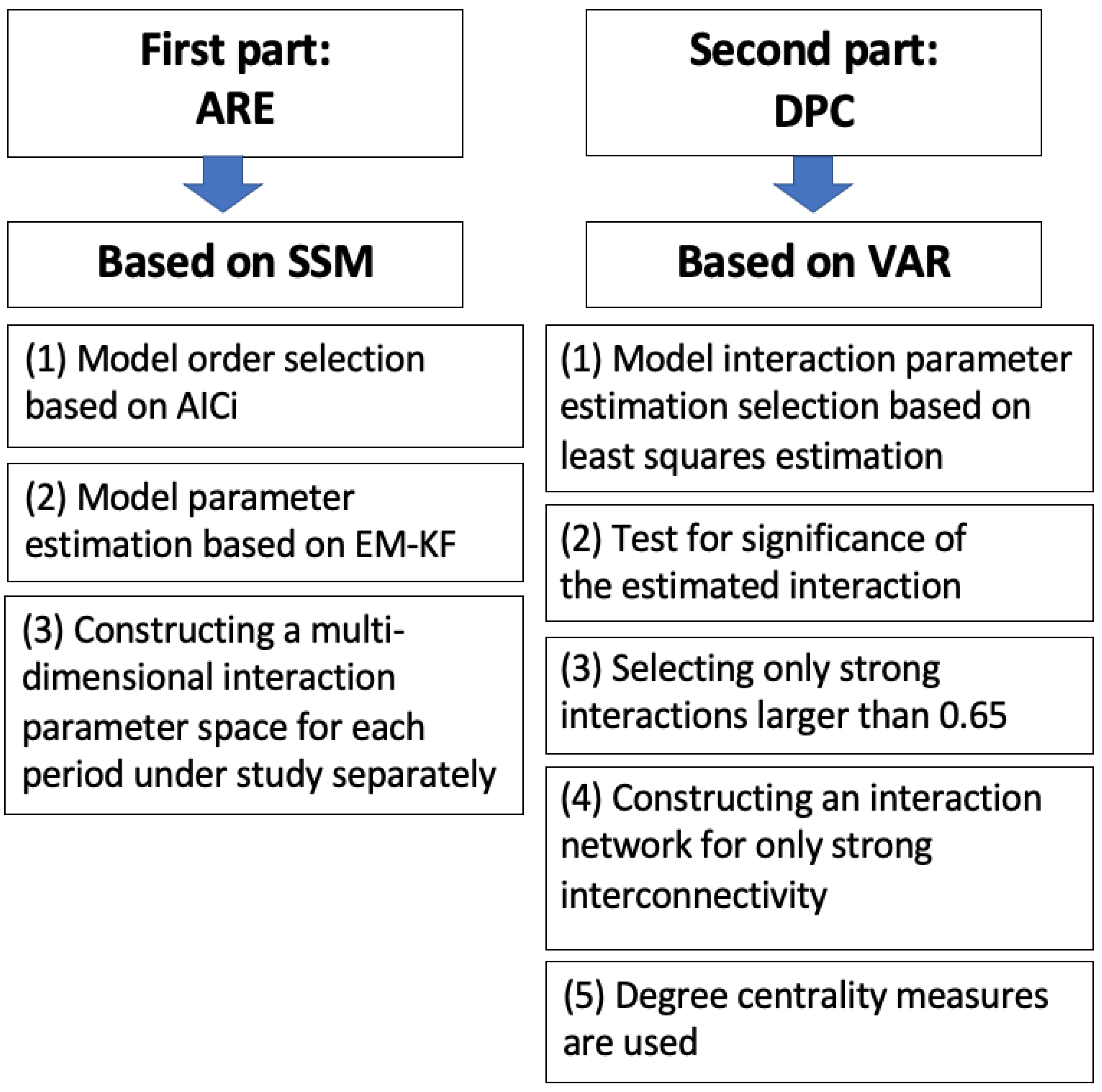
2. Methods
2.1. State Space Model (SSM)
2.2. Model Order Selection Criterion AICi
2.3. Expectation-Maximisation (EM) Algorithm and Kalman Filter (KL)
2.4. Granger Causality in the Time Domain: Directed Partial Correlation (DPC) [74]
- Generate B bootstrap surrogates (resamples) with the same length as the original data. A rough minimum of 1000 bootstrap surrogates is often sufficient to compute accurate confidence intervals, as has been suggested by Efron and Tibshirani [76]. Here, B is set to 10,000. The surrogates are generated using a non-parametric method—the amplitude-adjusted Fourier transform (AAFT) which was originally proposed by Theiler et al. (1992) [77,78]. This method works under the null hypothesis that the original data are generated from a stationary, Gaussian and linear stochastic process [79]. The algorithm for generating the surrogates is described as follows [79,80]:
- (a)
- The original data are re-scaled to a normal distribution. This is based on a simple rank ordering, which is performed by generating a time series with Gaussian distribution which is then sorted according to the original data.
- (b)
- A Fourier-transformed surrogate of the re-scaled data is constructed.
- (c)
- The final surrogate is scaled to the distribution of the original data by sorting the original data to the ranking of the Fourier-transformed surrogate.
The use of this algorithm is advantageous as it preserves the distribution, as well as approximately preserving the power spectrum (i.e., the autocorrelation structure), of the original data [79,80]. For the implementation of the AAFT method, we used the Tisean package (for details about the Tisean package, we refer to http://www.mpipks-dresden.mpg.de/tisean/) [78]. Note that the Tisean program performs the algorithm described above, iteratively, until no further improvement can be made [78]. - Estimate the DPC for each B bootstrap surrogates to yield a bootstrap sampling distribution, i.e. . To obtain the percentile bootstrap confidence interval for , the sampling distribution values of are sorted in ascending order. Then, the percent and percent points are chosen as the end points of the confidence interval, giving [] [81]. For a 95% confidence interval with , this would be approximately [].
- If the DPC value estimated from the original time series lies outside the confidence interval, then the value is considered to be significantly different from zero.
2.5. Degree-Centrality Measures
3. Application to American Stock Markets—Subprime Mortgage Crisis (2007–2008)
3.1. Data
- (a) 1/1/2006 to 30/6/2006 (first half of 2006)
- (b) 1/7/2006 to 30/6/2007 (second half of 2006 to first half of 2007)
- (c) 1/7/2007 to 31/12/2007 (second half of 2007)
- (d) 1/1/2008 to 31/12/2008 (2008)
- (e) 1/1/2009 to 31/12/2010 (2009–2010)
3.2. Model-Order Selection Criterion AIC
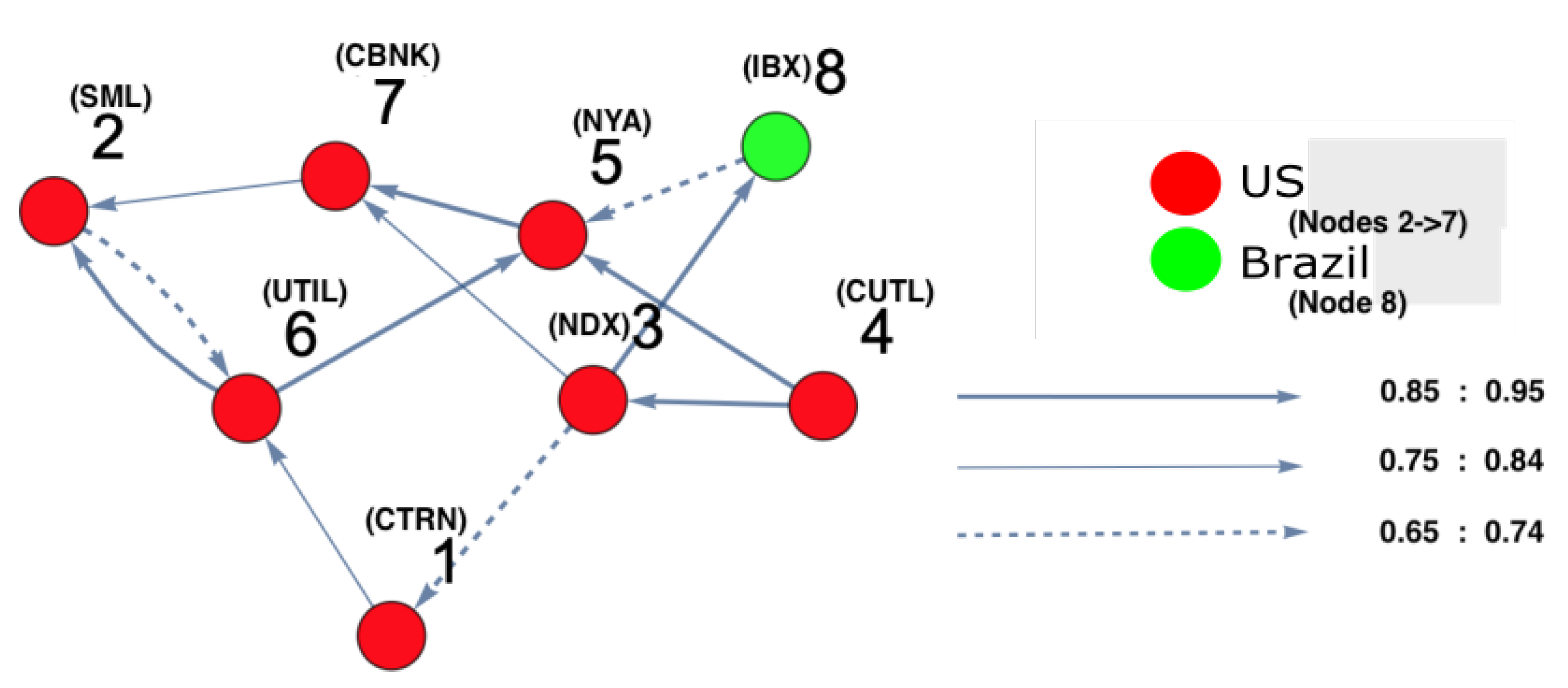
3.3. Results
4. Application to American Stock Markets: COVID-19 (2020)
4.1. Data
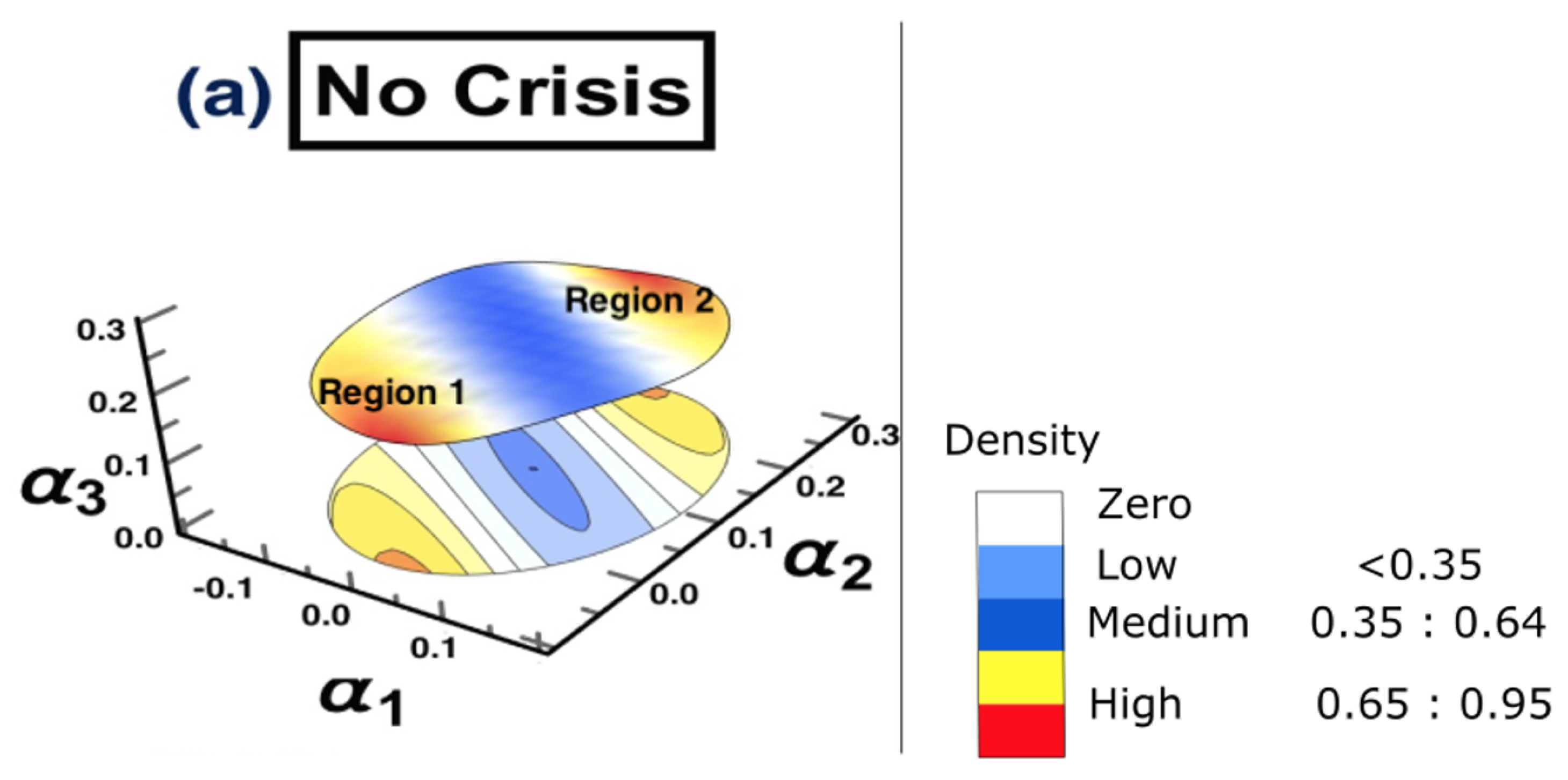
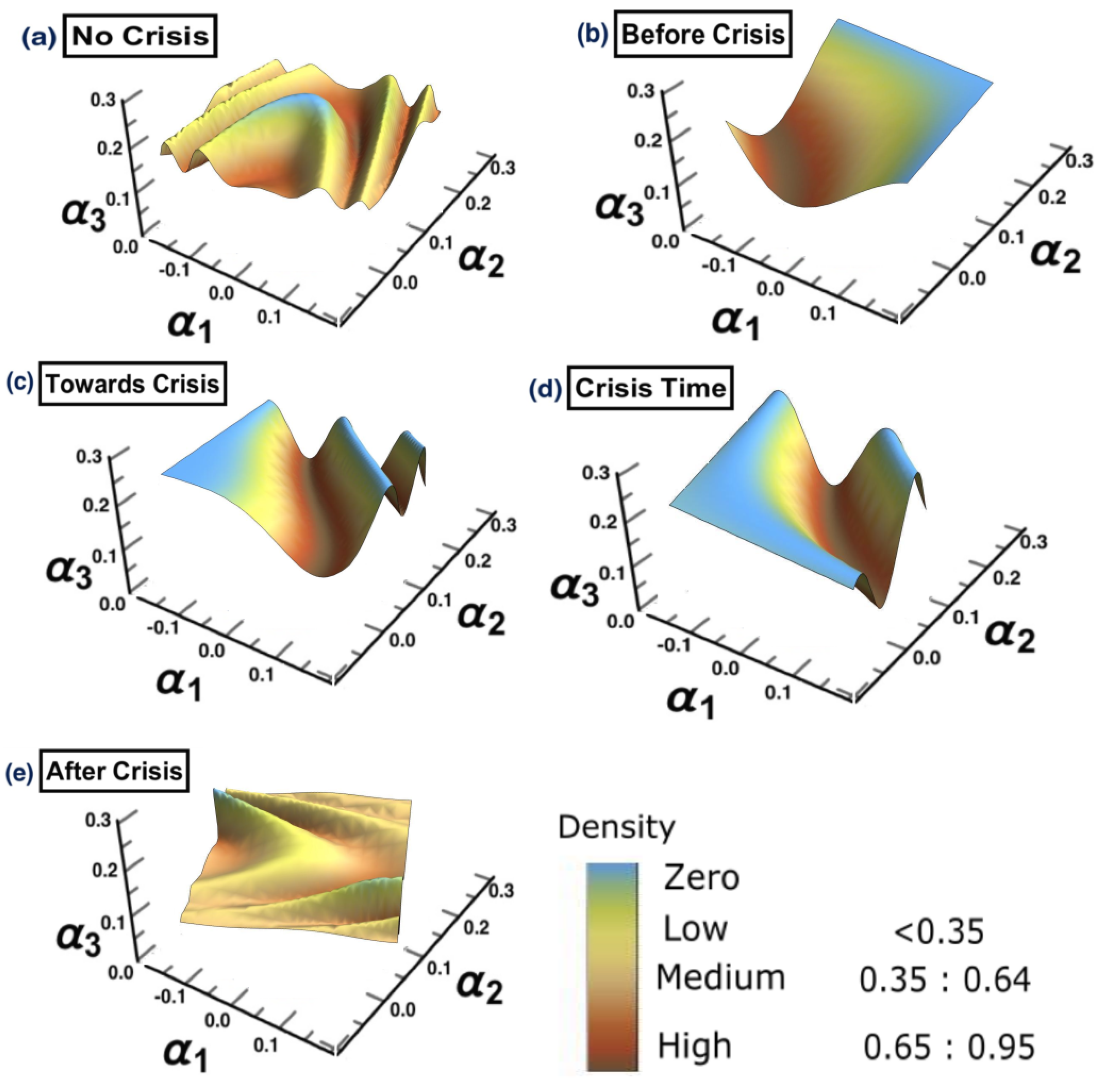
- (a) No crisis: 1/10/2018 to 31/3/2019
- (b) Before crisis: 1/4/2019 to 31/10/2019
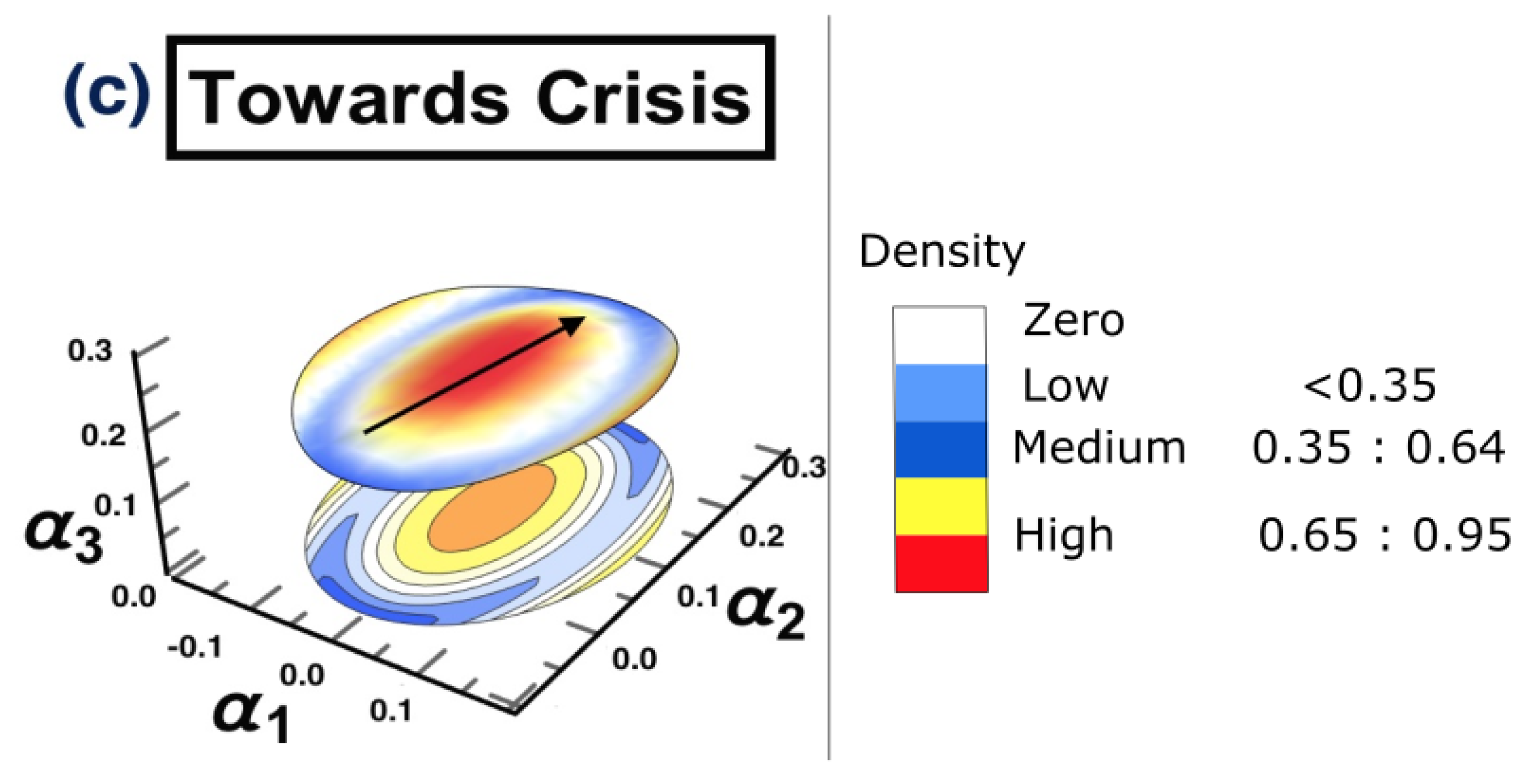
- (c) Towards crisis: 1/11/2019 to 28/2/2020
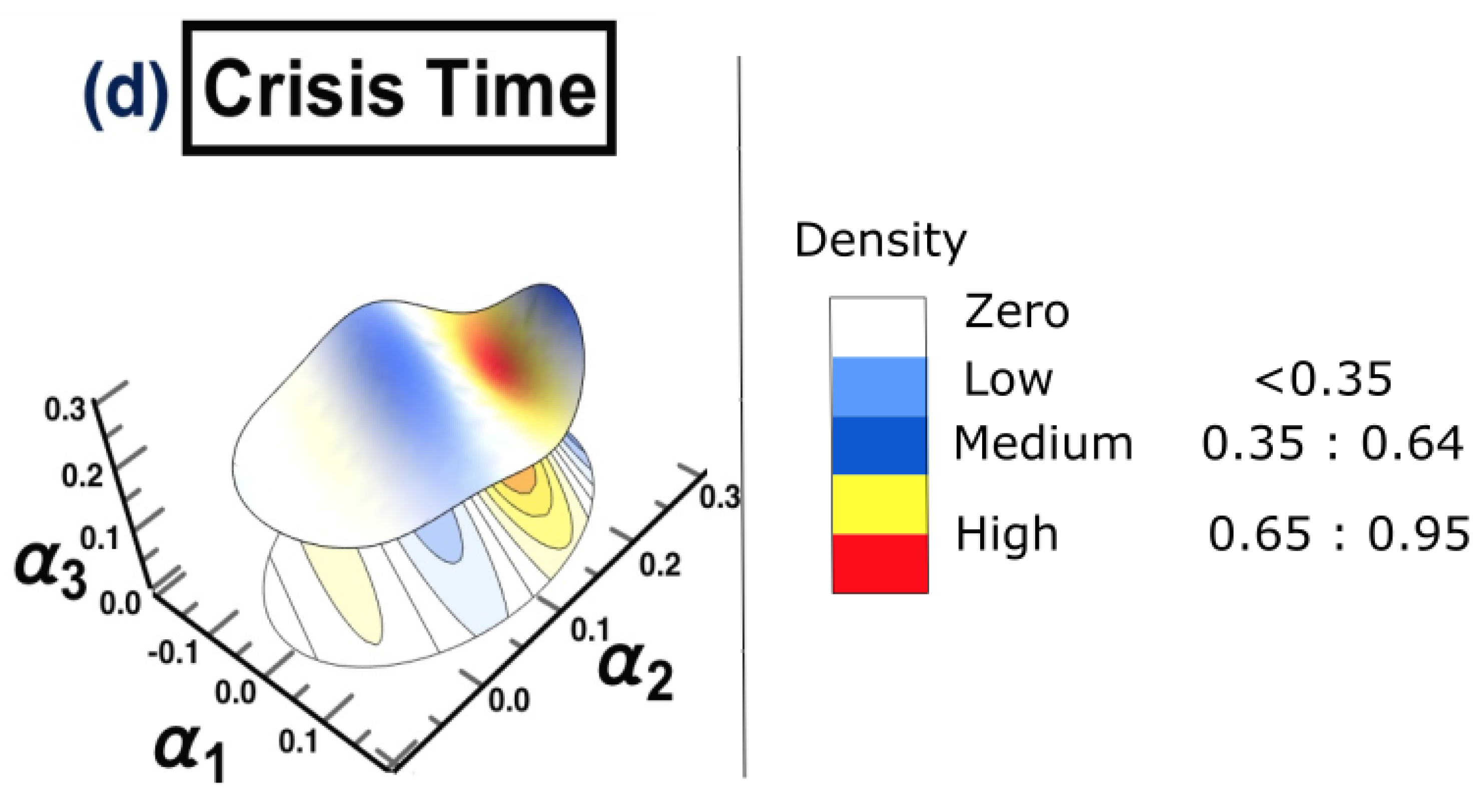
- (d) Crisis time: 1/3/2020 to 31/12/2020
- (e) After crisis: 2021
4.2. Model-Order Selection Criterion AIC
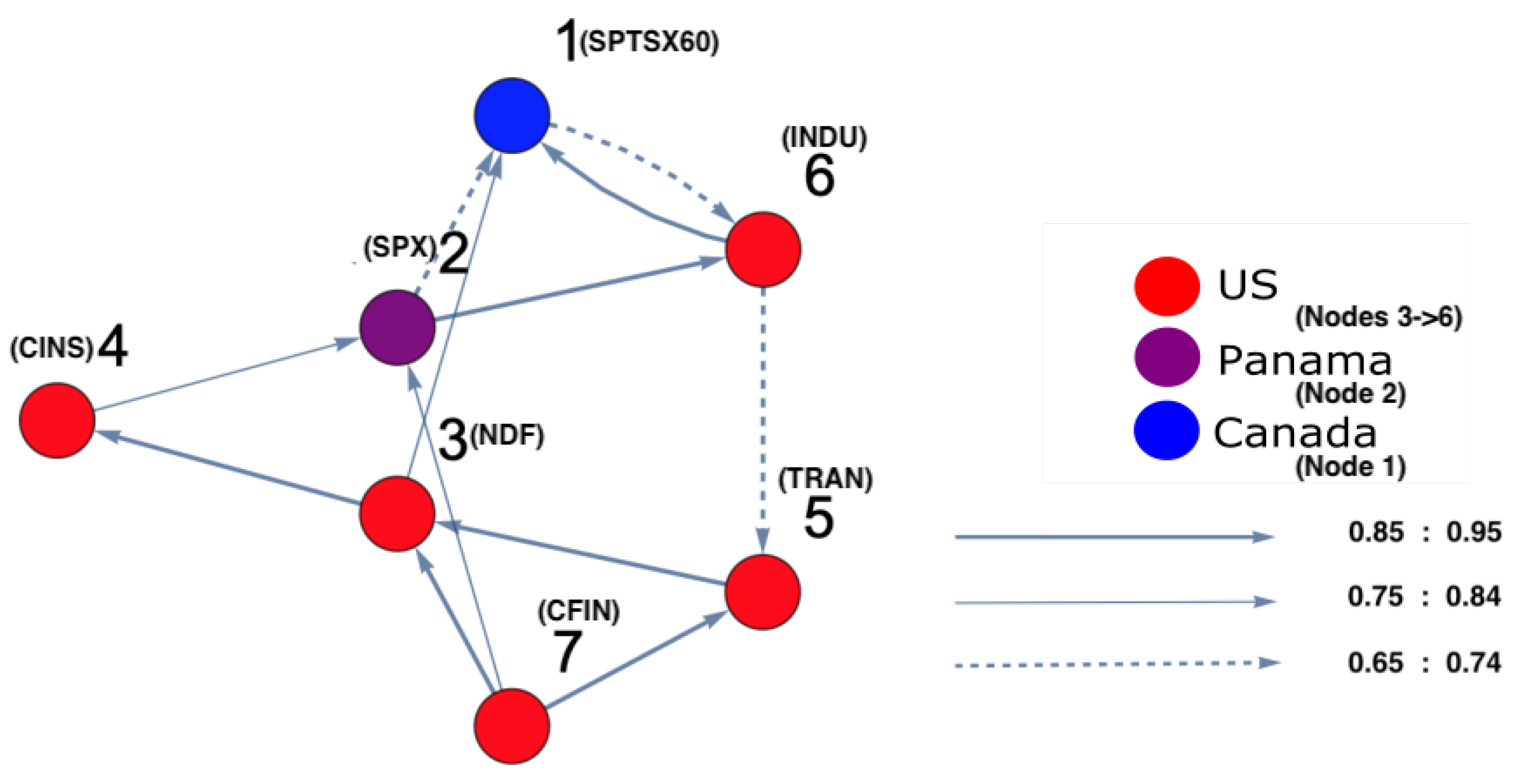
4.3. Results
5. Discussion and Conclusions
Funding
Data Availability Statement
Acknowledgments
Conflicts of Interest
Appendix A

| Country | Index |
|---|---|
| United States | 1- CTRN:IND NASDAQ TRANSPORTATION IXv |
| 2- SML:IND S & P 600 SMALLCAP INDEX | |
| 3- RTY:IND RUSSELL 2000 INDEX | |
| 4- NBI:IND NASDAQ BIOTECH INDEX | |
| 5- INDU:IND DOW JONES INDUS. AVG | |
| 6- CBNK:IND NASDAQ BANK INDEX | |
| 7- BBREIT:IND BBG U.S. REITS | |
| 8- NYA:IND NYSE COMPOSITE INDEX | |
| 9- NDX:IND NASDAQ 100 STOCK INDX | |
| 10- CFIN:IND NASDAQ OTHER FINANCIAL | |
| 11- CINS:IND NASDAQ INSURANCE INDEX | |
| 12- TRAN:IND DOW JONES TRANS. AVG | |
| 13- CUTL:IND NASDAQ TELECOMM INDEX | |
| 14- SPX:IND S & P 500 INDEX | |
| 15- CCMP:IND NASDAQ COMPOSITE INDEX | |
| 16- UTIL:IND DOW JONES UTILITY AVG | |
| 17- BKX:IND KBW BANK INDEX | |
| 18- RIY:IND RUSSELL 1000 INDEX | |
| 19- NDF:IND NASDAQ FINANCIAL INDEX | |
| 20- RAY:IND RUSSELL 3000 INDEX | |
| 21- IXK:IND NASDAQ COMPUTER INDEX | |
| 22- CIND:IND NASDAQ INDUSTRIAL INDEX | |
| Argentina | 23- BURCAP:IND S & P/BYMA Burcap TR ARS |
| 24- MAR:IND S & PMERVALArgentinaTR ARS | |
| 25- MERVAL:IND S & P MERVAL TR ARS | |
| Peru | 26- SPBL25PT:IND S & P/BVLLIMA25TRPEN |
| 27- SPBLPGPT:IND S & P/BVLPeruGeneralTRPEN | |
| Brazil | 28- IBX:IND BRAZIL IBrX INDEX |
| 29- IBOV:IND BRAZIL IBOVESPA INDEX | |
| Mexico | 30- INMEX:IND S & P/BMV INMEX |
| 31- MEXBOL:IND S & P/BMV IPC | |
| Canada | 32- SPTSX60:IND S & P/TSX 60 INDEX |
| 33- SPTSX:IND S & P/TSX COMPOSITE INDEX | |
| Chile | 34- IGPA:IND S & P/CLX IGPA (CLP) TR |
| 35- IPSA:IND S & P/CLX IPSA (CLP) TR | |
| Venezuela | 36- IBVC:IND VENEZUELA STOCK MKT INDX |
| Costa Rica | 37- CRSMBCT:IND BCT Corp Costa Rica Indx |
| Panama | 38- BVPSBVPS:IND Bolsa de Panama General |
| Jamaica | 39- JMSMX:IND JSE MARKET INDEX |
| Colombia | 40- COLCAP:IND COLOMBIA COLCAP INDEX |
| Bermuda | 41- BSX:IND BERMUDA STOCK EXCHANGE |
References
- Jin, L.; Myers, S.C. R2 around the world: New theory and new tests. J. Financ. Econ. 2006, 79, 257–292. [Google Scholar] [CrossRef] [Green Version]
- Xing, K.; Yang, X. How to detect crashes before they burst: Evidence from Chinese stock market. Phys. A Stat. Mech. Its Appl. 2019, 528, 121392. [Google Scholar] [CrossRef]
- Veraart, A.J.; Faassen, E.J.; Dakos, V.; van Nes, E.H.; Lürling, M.; Scheffer, M. Recovery rates reflect distance to a tipping point in a living system. Nature 2012, 481, 357–359. [Google Scholar] [CrossRef] [PubMed]
- Hutton, A.P.; Marcus, A.J.; Tehranian, H. Opaque financial reports, R2, and crash risk. J. Financ. Econ. 2009, 94, 67–86. [Google Scholar] [CrossRef]
- Gorvett, R. Why Stock Markets Crash: Critical Events in Complex Financial Systems. Princeton University Press-JSTOR. 2017. Available online: https://www.jstor.org/stable/j.ctt1h1htkg (accessed on 26 August 2022).
- Lenton, T.; Livina, V.; Dakos, V.; Van Nes, E.; Scheffer, M. Early warning of climate tipping points from critical slowing down: Comparing methods to improve robustness. Philos. Trans. R. Soc. A Math. Phys. Eng. Sci. 2012, 370, 1185–1204. [Google Scholar] [CrossRef]
- Chen, J.; Hong, H.; Stein, J.C. Forecasting crashes: Trading volume, past returns, and conditional skewness in stock prices. J. Financ. Econ. 2001, 61, 345–381. [Google Scholar] [CrossRef] [Green Version]
- Carpenter, S.R.; Cole, J.J.; Pace, M.L.; Batt, R.; Brock, W.A.; Cline, T.; Coloso, J.; Hodgson, J.R.; Kitchell, J.F.; Seekell, D.A.; et al. Early warnings of regime shifts: A whole-ecosystem experiment. Science 2011, 332, 1079–1082. [Google Scholar] [CrossRef] [Green Version]
- Gençay, R.; Gradojevic, N. The tale of two financial crises: An entropic perspective. Entropy 2017, 19, 244. [Google Scholar] [CrossRef]
- Bates, D.S. Post-’87 crash fears in the S&P 500 futures option market. J. Econom. 2000, 94, 181–238. [Google Scholar]
- Bates, D.S. The crash of ’87: Was it expected? The evidence from options markets. J. Financ. 1991, 46, 1009–1044. [Google Scholar] [CrossRef]
- Xing, Y.; Zhang, X.; Zhao, R. What does the individual option volatility smirk tell us about future equity returns? J. Financ. Quant. Anal. 2010, 45, 641–662. [Google Scholar] [CrossRef]
- Gradojevic, N. Brexit and foreign exchange market expectations: Could it have been predicted? Ann. Oper. Res. 2021, 297, 167–189. [Google Scholar] [CrossRef]
- Scheffer, M.; Carpenter, S.R.; Lenton, T.M.; Bascompte, J.; Brock, W.; Dakos, V.; Van de Koppel, J.; Van de Leemput, I.A.; Levin, S.A.; Van Nes, E.H.; et al. Anticipating critical transitions. Science 2012, 338, 344–348. [Google Scholar] [CrossRef] [PubMed] [Green Version]
- Huang, C.; Liu, S.; Yang, X.; Yang, X. Identification of crisis in the Chinese stock market based on complex network. Appl. Econ. Lett. 2022, 1–7. [Google Scholar] [CrossRef]
- Katsuragi, H. Evidence of multi-affinity in the Japanese stock market. Phys. A Stat. Mech. Its Appl. 2000, 278, 275–281. [Google Scholar] [CrossRef]
- Sun, X.; Chen, H.; Wu, Z.; Yuan, Y. Multifractal analysis of Hang Seng index in Hong Kong stock market. Phys. A Stat. Mech. Its Appl. 2001, 291, 553–562. [Google Scholar] [CrossRef]
- Sun, X.; Chen, H.; Yuan, Y.; Wu, Z. Predictability of multifractal analysis of Hang Seng stock index in Hong Kong. Phys. A Stat. Mech. Its Appl. 2001, 301, 473–482. [Google Scholar] [CrossRef]
- Tang, J.; Wang, J.; Huang, C.; Wang, G.; Wang, X. Subprime mortgage crisis detection in US foreign exchange rate market by multifractal analysis. In Proceedings of the 2008 The 9th International Conference for Young Computer Scientists, Hunan, China, 18–21 November 2008; pp. 2999–3004. [Google Scholar]
- Farrokhi, A.; Shirazi, F.; Hajli, N.; Tajvidi, M. Using artificial intelligence to detect crisis related to events: Decision making in B2B by artificial intelligence. Ind. Mark. Manag. 2020, 91, 257–273. [Google Scholar] [CrossRef]
- Waller, M.A.; Fawcett, S.E. Data science, predictive analytics, and big data: A revolution that will transform supply chain design and management. J. Bus. Logist. 2013, 34, 77–84. [Google Scholar] [CrossRef]
- Chatzis, S.P.; Siakoulis, V.; Petropoulos, A.; Stavroulakis, E.; Vlachogiannakis, N. Forecasting stock market crisis events using deep and statistical machine learning techniques. Expert Syst. Appl. 2018, 112, 353–371. [Google Scholar] [CrossRef]
- Deng, S.; Zhu, Y.; Duan, S.; Fu, Z.; Liu, Z. Stock Price Crash Warning in the Chinese Security Market Using a Machine Learning-Based Method and Financial Indicators. Systems 2022, 10, 108. [Google Scholar] [CrossRef]
- Huang, L.; Shi, P.; Zhu, H.; Chen, T. Early detection of emergency events from social media: A new text clustering approach. Nat. Hazards 2022, 111, 851–875. [Google Scholar] [CrossRef] [PubMed]
- Alharbi, A.; Lee, M. Crisis detection from Arabic tweets. In Proceedings of the 3rd Workshop on Arabic Corpus Linguistics, Cardiff, UK, October 2019; pp. 72–79. [Google Scholar]
- Mader, W.; Linke, Y.; Mader, M.; Sommerlade, L.; Timmer, J.; Schelter, B. A numerically efficient implementation of the expectation maximization algorithm for state space models. Appl. Math. Comput. 2014, 241, 222–232. [Google Scholar] [CrossRef] [Green Version]
- Schelter, B.; Mader, M.; Mader, W.; Sommerlade, L.; Platt, B.; Lai, Y.C.; Grebogi, C.; Thiel, M. Overarching framework for data-based modelling. EPL Europhys. Lett. 2014, 105, 30004. [Google Scholar] [CrossRef] [Green Version]
- Dempster, A.P.; Laird, N.M.; Rubin, D.B. Maximum likelihood from incomplete data via the EM algorithm. J. R. Stat. Soc. Ser. B Methodol. 1977, 39, 1–22. [Google Scholar]
- Kalman, R.E. A New Approach to Linear Filtering and Prediction Problems. Trans. ASME–J. Basic Eng. 1960, 82, 35–45. [Google Scholar] [CrossRef] [Green Version]
- Aldrich, J. RA Fisher and the making of maximum likelihood 1912–1922. Stat. Sci. 1997, 12, 162–176. [Google Scholar] [CrossRef]
- Shumway, R.H.; Stoffer, D.S. Time Series Analysis and Its Applications; Springer: Berlin/Heidelberg, Germany, 2000. [Google Scholar]
- Nalatore, H.; Ding, M.; Rangarajan, G. Mitigating the effects of measurement noise on Granger causality. Phys. Rev. E 2007, 75, 031123. [Google Scholar] [CrossRef] [Green Version]
- Nalatore, H.; Ding, M.; Rangarajan, G. Denoising neural data with state-space smoothing: Method and application. J. Neurosci. Methods 2009, 179, 131–141. [Google Scholar] [CrossRef] [Green Version]
- Sommerlade, L.; Thiel, M.; Mader, M.; Mader, W.; Timmer, J.; Platt, B.; Schelter, B. Assessing the strength of directed influences among neural signals: An approach to noisy data. J. Neurosci. Methods 2015, 239, 47–64. [Google Scholar] [CrossRef] [Green Version]
- Gao, L.; Sommerlade, L.; Coffman, B.; Zhang, T.; Stephen, J.M.; Li, D.; Wang, J.; Grebogi, C.; Schelter, B. Granger causal time-dependent source connectivity in the somatosensory network. Sci. Rep. 2015, 5, 1–10. [Google Scholar] [CrossRef] [PubMed] [Green Version]
- Frenzel, S.; Pompe, B. Partial mutual information for coupling analysis of multivariate time series. Phys. Rev. Lett. 2007, 99, 204101. [Google Scholar] [CrossRef] [PubMed]
- Paluš, M.; Stefanovska, A. Direction of coupling from phases of interacting oscillators: An information-theoretic approach. Phys. Rev. E 2003, 67, 055201. [Google Scholar] [CrossRef] [PubMed]
- Vejmelka, M.; Paluš, M. Inferring the directionality of coupling with conditional mutual information. Phys. Rev. E 2008, 77, 026214. [Google Scholar] [CrossRef] [Green Version]
- Paluš, M.; Vejmelka, M. Directionality of coupling from bivariate time series: How to avoid false causalities and missed connections. Phys. Rev. E 2007, 75, 056211. [Google Scholar] [CrossRef] [Green Version]
- Pompe, B.; Blidh, P.; Hoyer, D.; Eiselt, M. Using mutual information to measure coupling in the cardiorespiratory system. IEEE Eng. Med. Biol. Mag. 1998, 17, 32–39. [Google Scholar] [CrossRef]
- Arnold, M.; Milner, X.; Witte, H.; Bauer, R.; Braun, C. Adaptive AR modeling of nonstationary time series by means of Kalman filtering. IEEE Trans. Biomed. Eng. 1998, 45, 553–562. [Google Scholar] [CrossRef]
- Eichler, M. Graphical modelling of multivariate time series. Probab. Theory Relat. Fields 2012, 153, 233–268. [Google Scholar] [CrossRef] [Green Version]
- Eichler, M. Granger Causality Graphs for Multivariate Time Series. 2001. Available online: http://www.ub.uni-heidelberg.de/archiv/20749 (accessed on 26 August 2022).
- Halliday, D.; Rosenberg, J. On the application, estimation and interpretation of coherence and pooled coherence. J. Neurosci. Methods 2000, 100, 173–174. [Google Scholar] [CrossRef]
- Dahlhaus, R. Graphical interaction models for multivariate time series. Metrika 2000, 51, 157–172. [Google Scholar] [CrossRef] [Green Version]
- Nolte, G.; Ziehe, A.; Nikulin, V.V.; Schlögl, A.; Krämer, N.; Brismar, T.; Müller, K.R. Robustly estimating the flow direction of information in complex physical systems. Phys. Rev. Lett. 2008, 100, 234101. [Google Scholar] [CrossRef] [PubMed] [Green Version]
- Arnhold, J.; Grassberger, P.; Lehnertz, K.; Elger, C.E. A robust method for detecting interdependences: Application to intracranially recorded EEG. Phys. D Nonlinear Phenom. 1999, 134, 419–430. [Google Scholar] [CrossRef]
- Chicharro, D.; Andrzejak, R.G. Reliable detection of directional couplings using rank statistics. Phys. Rev. E 2009, 80, 026217. [Google Scholar] [CrossRef] [PubMed] [Green Version]
- Romano, M.C.; Thiel, M.; Kurths, J.; Grebogi, C. Estimation of the direction of the coupling by conditional probabilities of recurrence. Phys. Rev. E 2007, 76, 036211. [Google Scholar] [CrossRef] [Green Version]
- Sims, C.A. Macroeconomics and reality. Econometrica 1980, 48, 1–4. [Google Scholar] [CrossRef] [Green Version]
- Granger, C.W.J. Investigating causal relations by econometric models and cross-spectral methods. Econom. J. Econom. Soc. 1969, 37, 424–438. [Google Scholar] [CrossRef]
- Granger, C.W.J. Some recent development in a concept of causality. J. Econom. 1988, 39, 199–211. [Google Scholar] [CrossRef]
- Granger, C.W.J. Economic processes involving feedback. Inf. Control 1963, 6, 28–48. [Google Scholar] [CrossRef] [Green Version]
- Granger, C.W.J. Testing for causality: A personal viewpoint. J. Econ. Dyn. Control 1980, 2, 329–352. [Google Scholar] [CrossRef]
- Schelter, B.; Timmer, J.; Eichler, M. Assessing the strength of directed influences among neural signals using renormalized partial directed coherence. J. Neurosci. Methods 2009, 179, 121–130. [Google Scholar] [CrossRef]
- Eichler, M. A graphical approach for evaluating effective connectivity in neural systems. Philos. Trans. R. Soc. Lond. B Biol. Sci. 2005, 360, 953–967. [Google Scholar] [CrossRef] [PubMed] [Green Version]
- Bessler, D.A.; Yang, J. The structure of interdependence in international stock markets. J. Int. Money Financ. 2003, 22, 261–287. [Google Scholar] [CrossRef]
- Glezakos, M.; Merika, A.; Kaligosfiris, H. Interdependence of major world stock exchanges: How is the Athens stock exchange affected? Int. Res. J. Financ. Econ. 2007, 7, 25–39. [Google Scholar]
- Égert, B.; Kočenda, E. Interdependence between Eastern and Western European stock markets: Evidence from intraday data. Econ. Syst. 2007, 31, 184–203. [Google Scholar] [CrossRef]
- Martens, M.; Poon, S.H. Return synchronization and daily correlation dynamics between international stock markets. J. Bank. Financ. 2001, 25, 1805–1827. [Google Scholar] [CrossRef]
- Sandoval, L. To lag or not to lag? how to compare indices of stock markets that operate on different times. Phys. A Stat. Mech. Its Appl. 2014, 403, 227–243. [Google Scholar] [CrossRef] [Green Version]
- Sandoval, L. Correlation of financial markets in times of crisis. Phisica A 2014, 391, 187–208. [Google Scholar] [CrossRef] [Green Version]
- Elsegai, H.; Shiells, H.; Thiel, M.; Schelter, B. Network inference in the presence of latent confounders: The role of instantaneous causalities. J. Neurosci. Methods 2015, 245, 91–106. [Google Scholar] [CrossRef]
- Akaike, H. A new look at the statistical model identification. IEEE Trans. Autom. Control 1974, 19, 716–723. [Google Scholar] [CrossRef]
- Sugiura, N. Further analysts of the data by akaike’s information criterion and the finite corrections: Further analysts of the data by akaike’s. Commun. Stat.-Theory Methods 1978, 7, 13–26. [Google Scholar] [CrossRef]
- Hurvich, C.M.; Tsai, C.L. Regression and time series model selection in small samples. Biometrika 1989, 76, 297–307. [Google Scholar] [CrossRef]
- Hurvich, C.M.; Shumway, R.; Tsai, C.L. Improved estimators of Kullback–Leibler information for autoregressive model selection in small samples. Biometrika 1990, 77, 709–719. [Google Scholar]
- Bengtsson, T.; Cavanaugh, J.E. An improved Akaike information criterion for state-space model selection. Comput. Stat. Data Anal. 2006, 50, 2635–2654. [Google Scholar] [CrossRef]
- Sommerlade, L.; Thiel, M.; Platt, B.; Plano, A.; Riedel, G.; Grebogi, C.; Timmer, J.; Schelter, B. Inference of Granger causal time-dependent influences in noisy multivariate time series. J. Neurosci. Methods 2012, 203, 173–185. [Google Scholar] [CrossRef] [PubMed]
- Killmann, M.; Sommerlade, L.; Mader, W.; Timmer, J.; Schelter, B. Inference of time-dependent causal influences in Networks. Biomed. Eng. Tech. 2012, 57, 387–390. [Google Scholar] [CrossRef] [Green Version]
- Shumway, R.H.; Stoffer, D.S. An approach to time series smoothing and forecasting using the EM algorithm. J. Time Ser. Anal. 1982, 3, 253–264. [Google Scholar] [CrossRef]
- Welch, G.; Bishop, G. An Introduction to the Kalman Filter; Proc of SIGGRAPH, Course; University of North Carolina: Chapel Hill, NC, USA, 2001; Volume 8, pp. 23175–27599. [Google Scholar]
- Khan, M.E.; Dutt, D.N. An expectation-maximization algorithm based kalman smoother approach for event-related desynchronization (ERD) estimation from EEG. Biomed. Eng. IEEE Trans. 2007, 54, 1191–1198. [Google Scholar] [CrossRef] [Green Version]
- Elsegai, H. Granger-causality inference in the presence of gaps: An equidistant missing-data problem for non-synchronous recorded time series data. Phys. A Stat. Mech. Its Appl. 2019, 523, 839–851. [Google Scholar] [CrossRef]
- Lütkepohl, H. New Introduction to Multiple Time Series Analysis; Springer: Berlin/Heidelberg, Germany, 2007. [Google Scholar]
- Efron, B.; Tibshirani, R. Bootstrap methods for standard errors, confidence intervals, and other measures of statistical accuracy. Stat. Sci. 1986, 54–75. Available online: https://www.jstor.org/stable/2245500 (accessed on 26 August 2022). [CrossRef]
- Theiler, J.; Eubank, S.; Longtin, A.; Galdrikian, B.; Farmer, J.D. Testing for nonlinearity in time series: The method of surrogate data. Phys. D Nonlinear Phenom. 1992, 58, 77–94. [Google Scholar] [CrossRef] [Green Version]
- Hegger, R.; Kantz, H.; Schreiber, T. Practical implementation of nonlinear time series methods: The TISEAN package. Chaos Interdiscip. J. Nonlinear Sci. 1999, 9, 413–435. [Google Scholar] [CrossRef] [PubMed] [Green Version]
- Dolan, K.T.; Spano, M.L. Surrogate for nonlinear time series analysis. Phys. Rev. E 2001, 64, 046128. [Google Scholar] [CrossRef] [PubMed] [Green Version]
- Schreiber, T.; Schmitz, A. Surrogate time series. Phys. D Nonlinear Phenom. 2000, 142, 346–382. [Google Scholar] [CrossRef] [Green Version]
- Balamurali, S. Bootstrap confidence limits for short-run capability indices. Qual. Eng. 2003, 15, 643–648. [Google Scholar] [CrossRef]
- Hansen, D.L.; Shneiderman, B.; Smith, M.A.; Himelboim, I. Social network analysis: Measuring, mapping, and modeling collections of connections. Anal. Soc. Media Netw. NodeXL 2020, 31–51. [Google Scholar] [CrossRef]
- Serrat, O. Social network analysis. In Knowledge Solutions; Springer: Berlin/Heidelberg, Germany, 2017; pp. 39–43. [Google Scholar]
- Yahoo Finance Database. Available online: http://finance.yahoo.com/world-indices (accessed on 5 December 2021).
- Bikhchandani, S.; Sharma, S. Herd behavior in financial markets. IMF Staff Pap. 2000, 47, 279–310. [Google Scholar]
- Chang, E.C.; Cheng, J.W.; Khorana, A. An examination of herd behavior in equity markets: An international perspective. J. Bank. Financ. 2000, 24, 1651–1679. [Google Scholar] [CrossRef]
- Rakshit, B.; Neog, Y. Effects of the COVID-19 pandemic on stock market returns and volatilities: Evidence from selected emerging economies. Stud. Econ. Financ. 2021. [Google Scholar] [CrossRef]
- Hatmanu, M.; Cautisanu, C. The impact of COVID-19 pandemic on stock market: Evidence from Romania. Int. J. Environ. Res. Public Health 2021, 18, 9315. [Google Scholar] [CrossRef]
- Ashraf, B.N. Economic impact of government interventions during the COVID-19 pandemic: International evidence from financial markets. J. Behav. Exp. Financ. 2020, 27, 100371. [Google Scholar] [CrossRef]
- Lyócsa, Š.; Baumöhl, E.; Vỳrost, T.; Molnár, P. Fear of the coronavirus and the stock markets. Financ. Res. Lett. 2020, 36, 101735. [Google Scholar] [CrossRef] [PubMed]
- Liu, H.; Manzoor, A.; Wang, C.; Zhang, L.; Manzoor, Z. The COVID-19 outbreak and affected countries stock markets response. Int. J. Environ. Res. Public Health 2020, 17, 2800. [Google Scholar] [CrossRef] [PubMed] [Green Version]
- Jabeen, S.; Farhan, M.; Zaka, M.A.; Fiaz, M.; Farasat, M. COVID and World Stock Markets: A Comprehensive Discussion. Front. Psychol. 2022, 4837. [Google Scholar] [CrossRef] [PubMed]
- Tiwari, A.K.; Abakah, E.J.A.; Karikari, N.K.; Gil-Alana, L.A. The outbreak of COVID-19 and stock market liquidity: Evidence from emerging and developed equity markets. N. Am. J. Econ. Financ. 2022, 62, 101735. [Google Scholar] [CrossRef]


| Order | AICi |
|---|---|
| 1 | 49 |
| 2 | 42 |
| 3 | 732 |
| 4 | 34 |
| 5 | 20 |
| 6 | 5 |
| 7 | 0 |
| 8 | 0 |
| 9 | 0 |
| 10 | 0 |
| Node Number | Out-Degree | In-Degree |
|---|---|---|
| 1 | 3 | 0 |
| 2 | 2 | 2 |
| 3 | 1 | 3 |
| 4 | 1 | 1 |
| 5 | 3 | 2 |
| 6 | 1 | 2 |
| 7 | 0 | 1 |
| 8 | 1 | 3 |
| 9 | 2 | 2 |
| 10 | 3 | 1 |
| 11 | 2 | 2 |
| 12 | 1 | 1 |
| 13 | 1 | 1 |
| 14 | 2 | 1 |
| 15 | 1 | 2 |
| 16 | 3 | 1 |
| 17 | 0 | 2 |
| Node Number | Out-Degree | In-Degree |
|---|---|---|
| 1 | 3 | 0 |
| 2 | 2 | 2 |
| 3 | 2 | 3 |
| 4 | 1 | 1 |
| 5 | 3 | 2 |
| 6 | 1 | 3 |
| 7 | 1 | 1 |
| 8 | 1 | 4 |
| 9 | 2 | 2 |
| 10 | 3 | 1 |
| 11 | 2 | 2 |
| 12 | 1 | 1 |
| 13 | 1 | 1 |
| 14 | 2 | 1 |
| 15 | 1 | 2 |
| 16 | 3 | 1 |
| 17 | 0 | 2 |
| Order | AICi |
|---|---|
| 1 | 53 |
| 2 | 34 |
| 3 | 945 |
| 4 | 56 |
| 5 | 28 |
| 6 | 3 |
| 7 | 0 |
| 8 | 0 |
| 9 | 0 |
| 10 | 0 |
Disclaimer/Publisher’s Note: The statements, opinions and data contained in all publications are solely those of the individual author(s) and contributor(s) and not of MDPI and/or the editor(s). MDPI and/or the editor(s) disclaim responsibility for any injury to people or property resulting from any ideas, methods, instructions or products referred to in the content. |
© 2022 by the author. Licensee MDPI, Basel, Switzerland. This article is an open access article distributed under the terms and conditions of the Creative Commons Attribution (CC BY) license (https://creativecommons.org/licenses/by/4.0/).
Share and Cite
Elsegai, H. Improving the Process of Early-Warning Detection and Identifying the Most Affected Markets: Evidence from Subprime Mortgage Crisis and COVID-19 Outbreak—Application to American Stock Markets. Entropy 2023, 25, 70. https://doi.org/10.3390/e25010070
Elsegai H. Improving the Process of Early-Warning Detection and Identifying the Most Affected Markets: Evidence from Subprime Mortgage Crisis and COVID-19 Outbreak—Application to American Stock Markets. Entropy. 2023; 25(1):70. https://doi.org/10.3390/e25010070
Chicago/Turabian StyleElsegai, Heba. 2023. "Improving the Process of Early-Warning Detection and Identifying the Most Affected Markets: Evidence from Subprime Mortgage Crisis and COVID-19 Outbreak—Application to American Stock Markets" Entropy 25, no. 1: 70. https://doi.org/10.3390/e25010070