

Multi-Level Thresholding Image Segmentation Based on Improved Slime Mould Algorithm and Symmetric Cross-Entropy
Abstract
:1. Introduction
2. Slime Mould Algorithm
3. The Proposed Method
3.1. Elite Opposition-Based Learning
3.2. The Adaptive Probability Threshold
3.3. The Historical Leader
3.4. Pseudo-Code of ISMA
| Algorithm 1 Pseudo-code of ISMA |
| Initialize the parameters popsize, Max_iteraition |
| Initialize the positions of the slime mould |
| While (t ≤ Max_iteraition) |
| Calculate the fitness of all the slime mould |
| Update bestFitness, Xb |
| Calculate the W by Equation (4) |
| For each search portion, |
| Update p by Equation (8) |
| Update positions by Equation (9) |
| End For |
| t = t + 1 |
| End While |
| Return bestFitness, Xb |
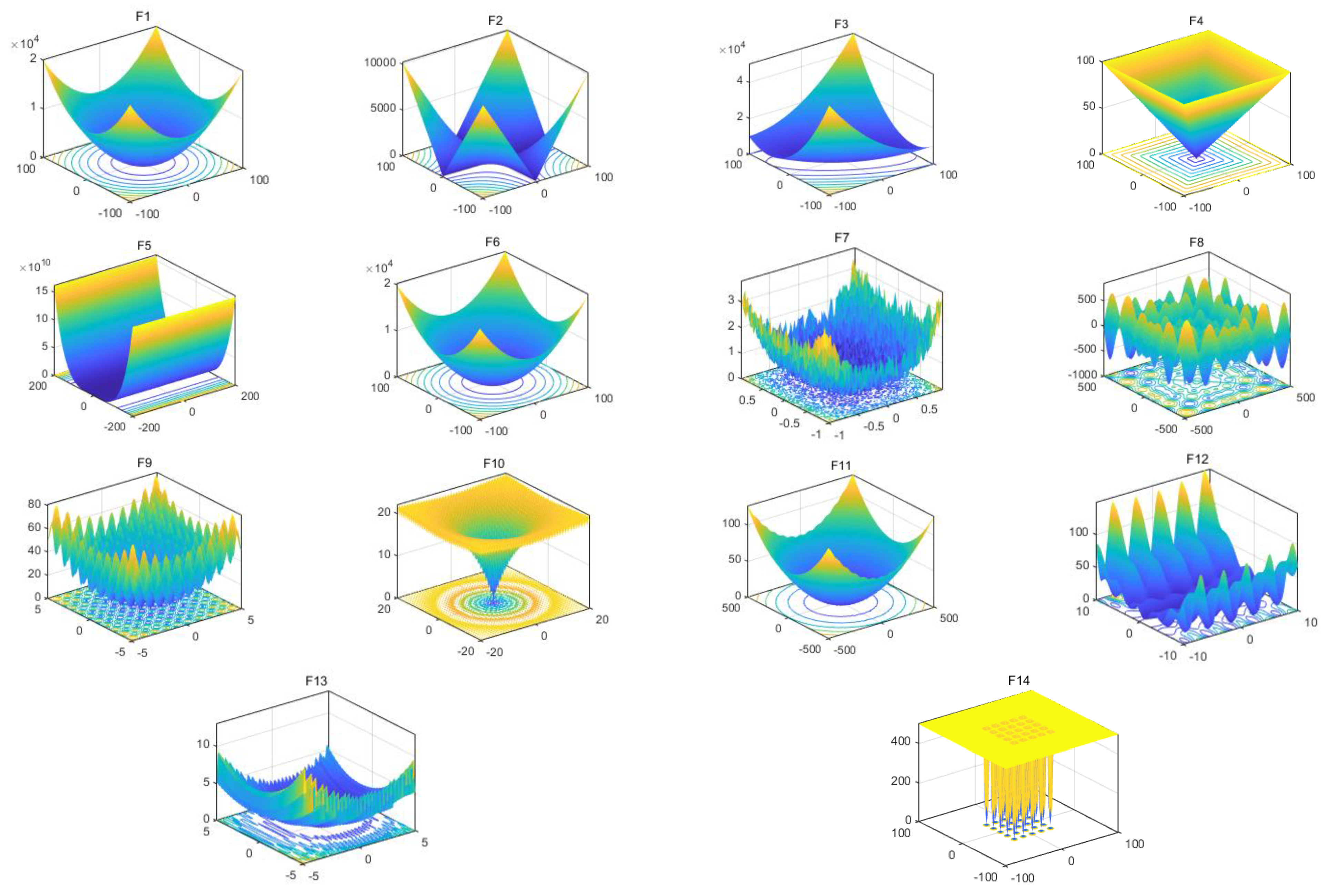
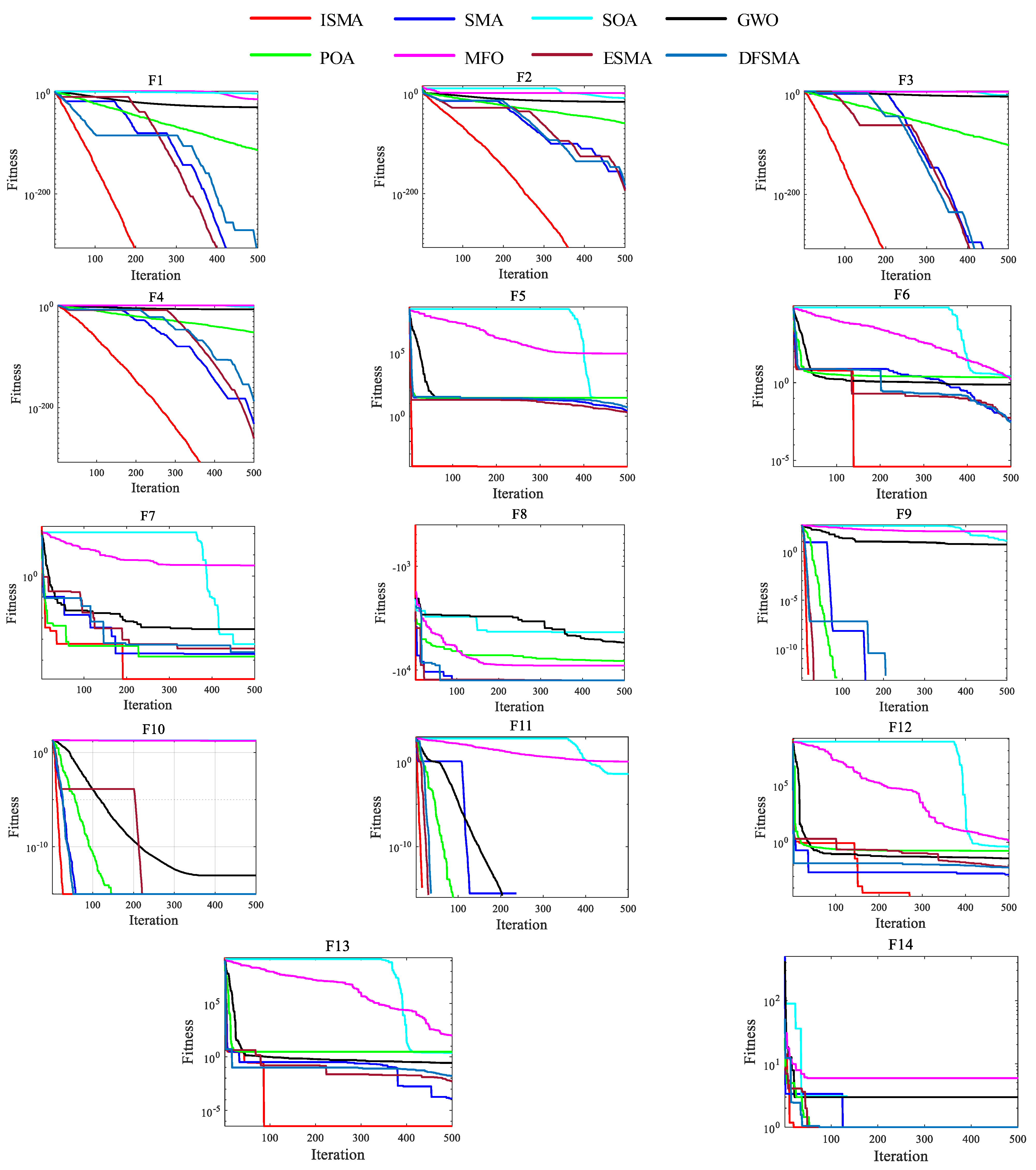
4. ISMA Performance Evaluation Experiments and Analysis
5. Multi-Threshold Segmentation
5.1. Symmetric Cross-Entropy Threshold Segmentation
5.2. Multi-Level Threshold Segmentation Based on ISMA and Symmetric Cross-Entropy
- (a)
- Read the image to be segmented (grayscale image).
- (b)
- Find the grayscale histogram of the image.
- (c)
- Initialize the parameters of ISMA, the size of the population of slime mould (n), the maximum number of iterations (max_t), the initial values of the upper bound (LB) and lower bound (UB), and the number of desired partition thresholds (d).
- (d)
- Find the optimal fitness value using symmetric cross-entropy as the ISMA objective function.
- (e)
- If ISMA reaches the maximum number of iterations max_t, the optimization is completed, and the slime mould location information regarding the best fitness is returned, which is the best segmentation threshold. Otherwise, skip to step (d).
- (f)
- Perform grayscale image segmentation with the best threshold and obtain the segmented image.
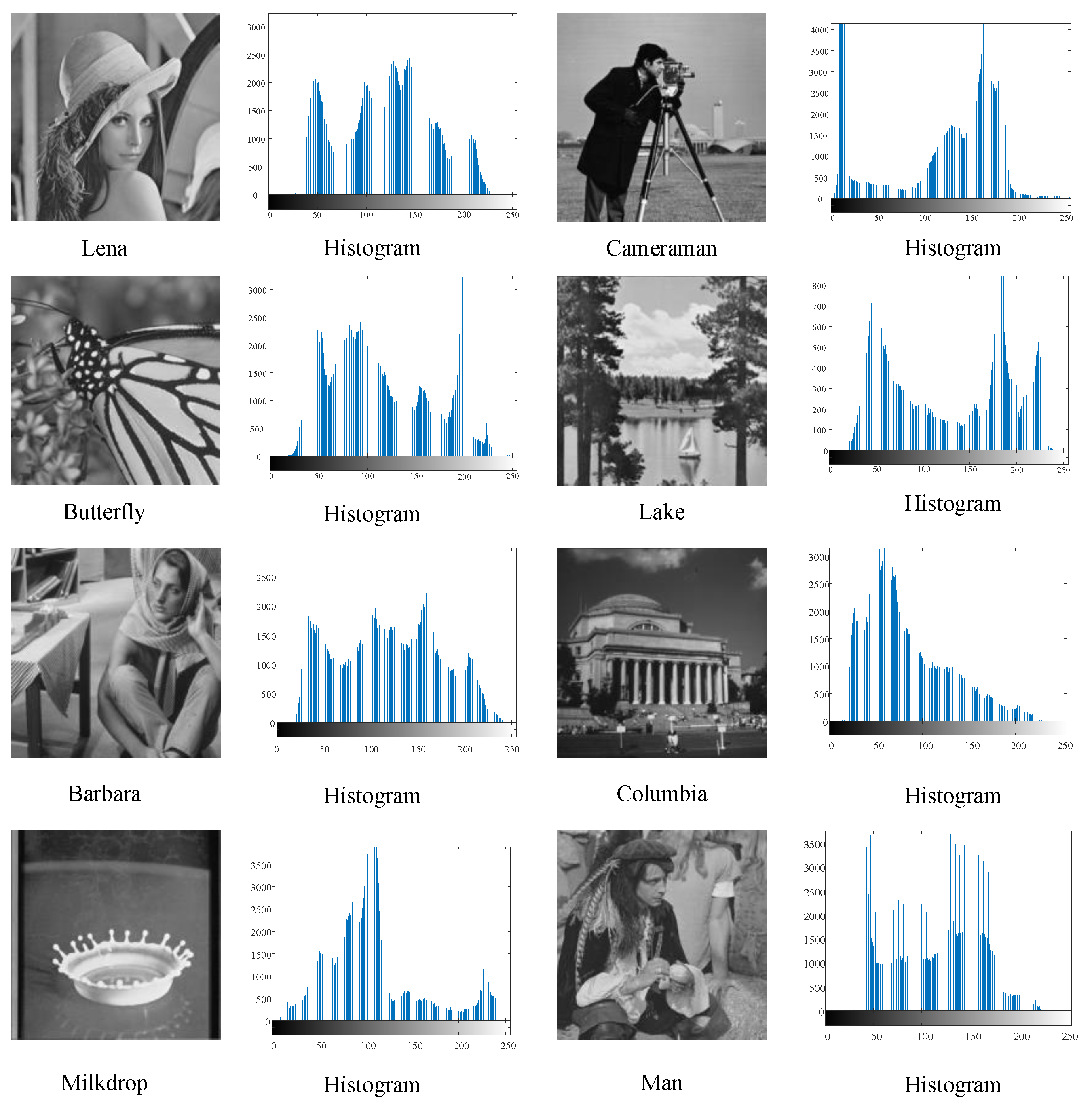
6. Threshold Segmentation Experiment Results and Analysis
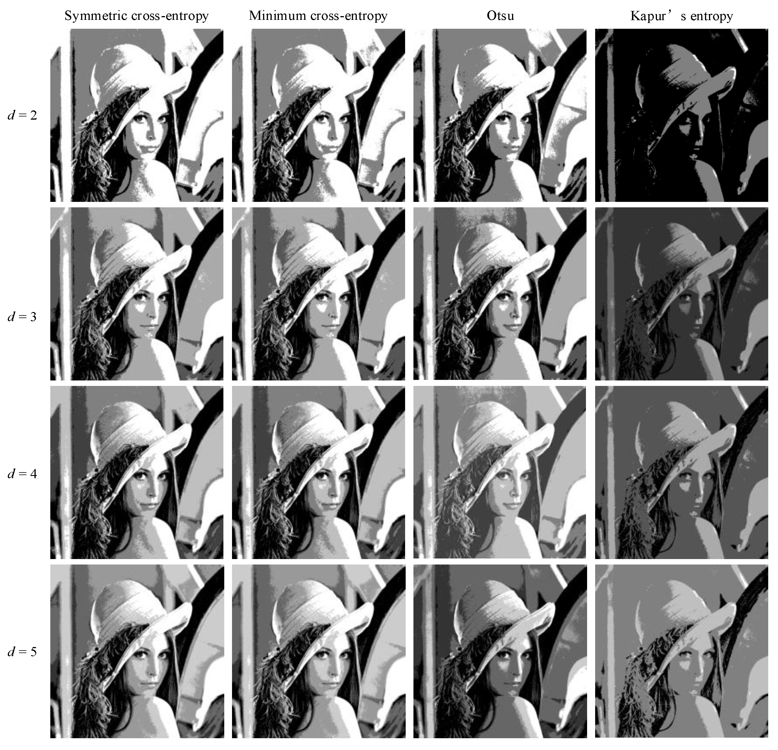
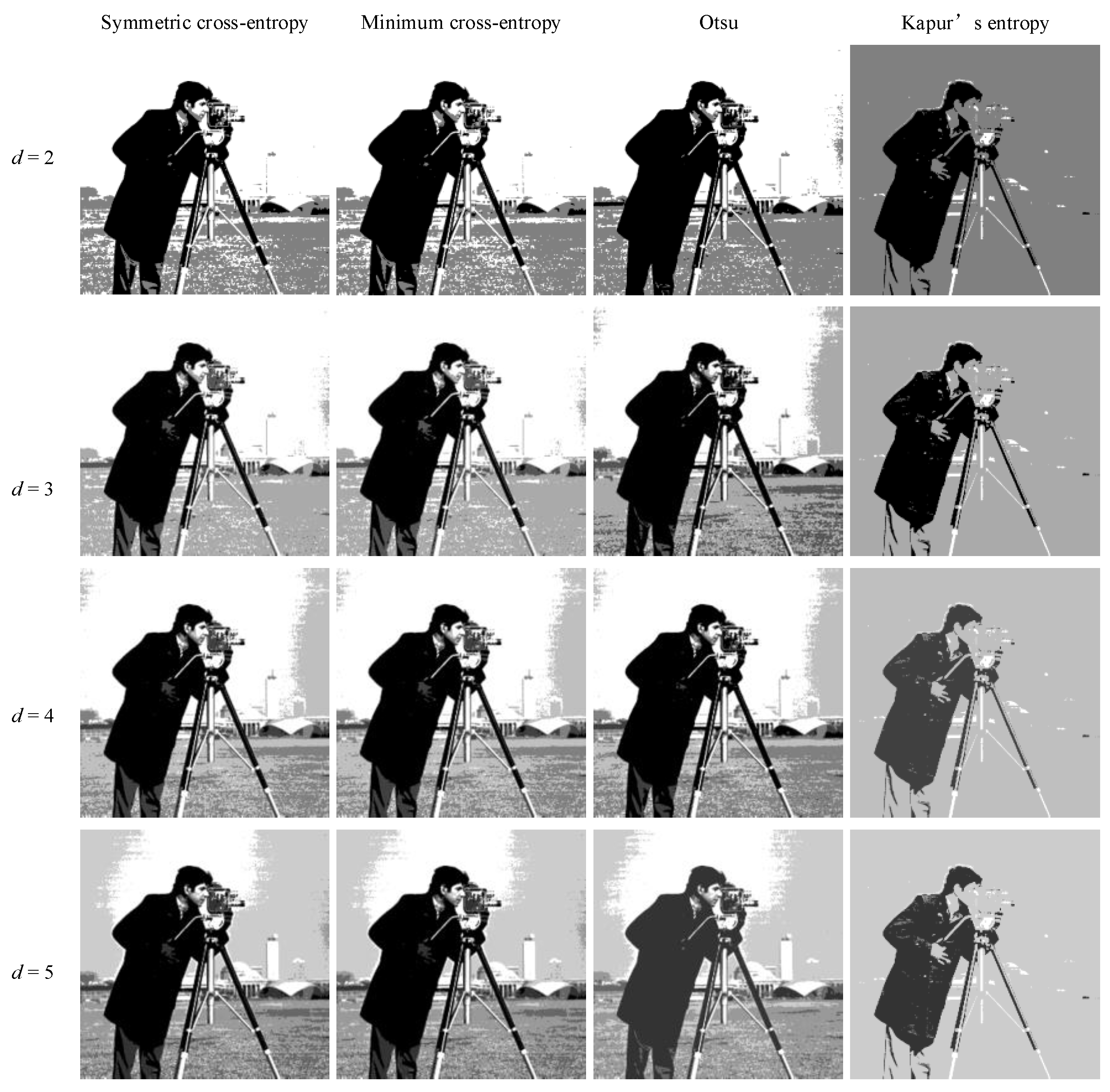
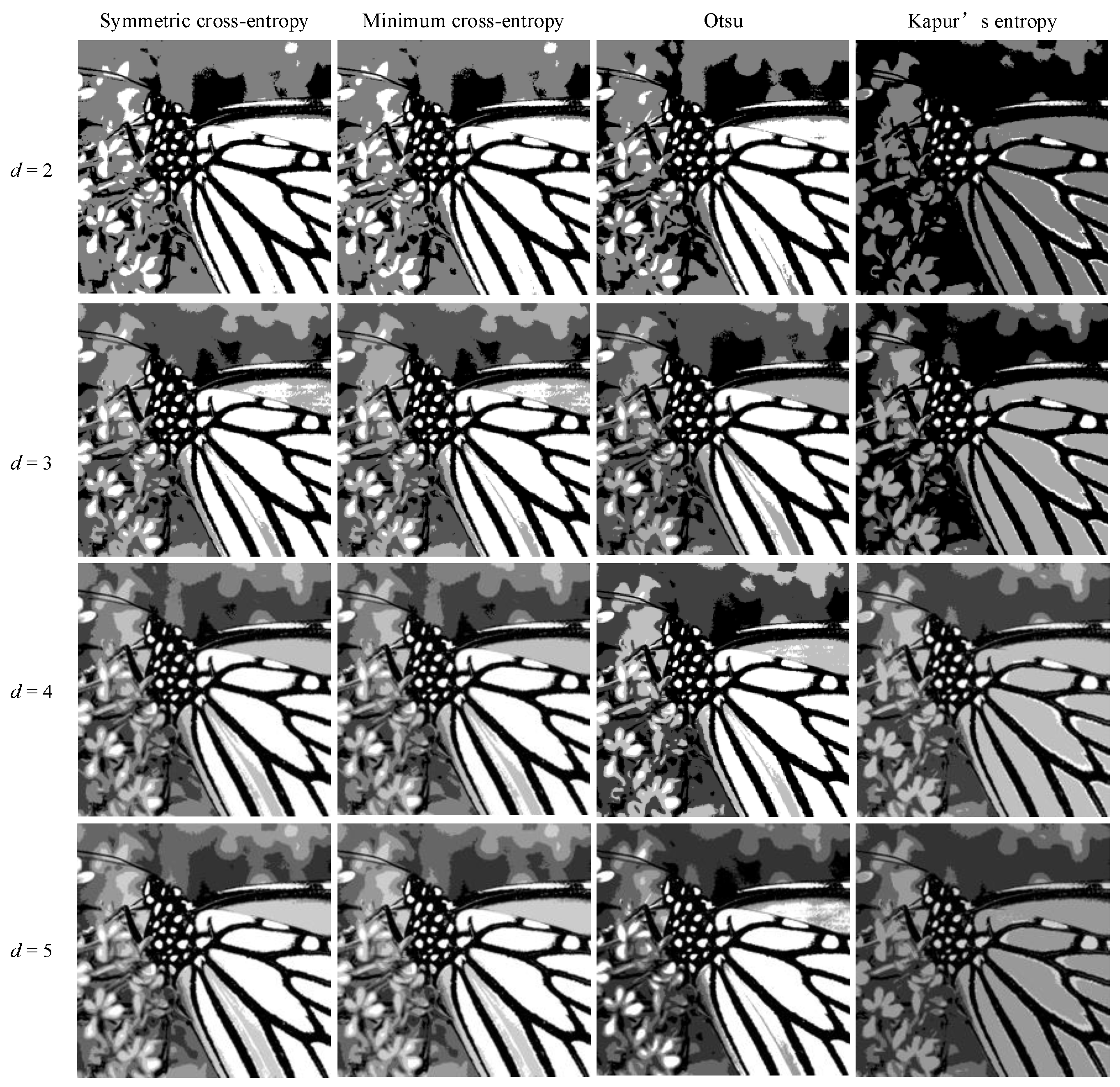
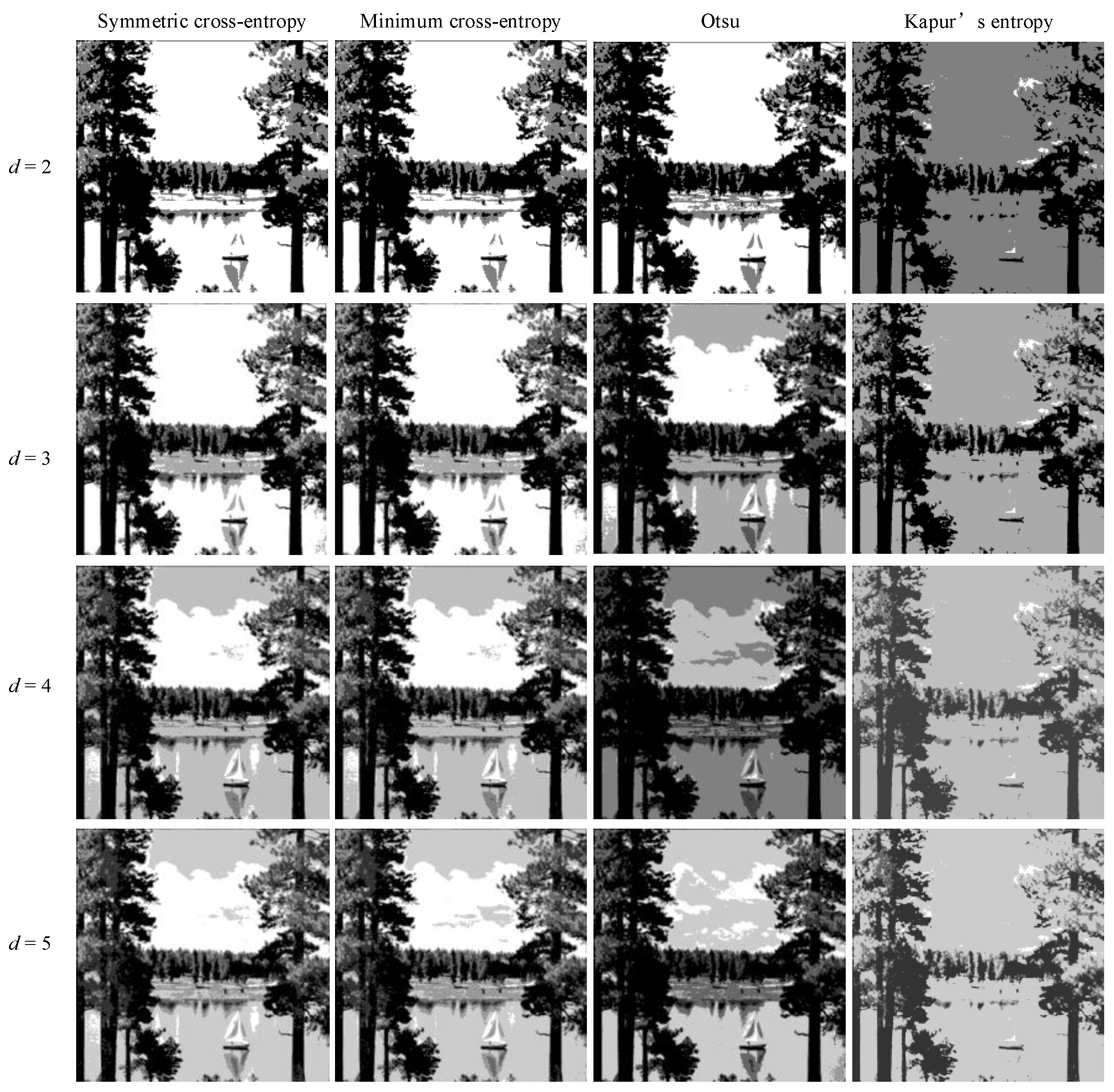
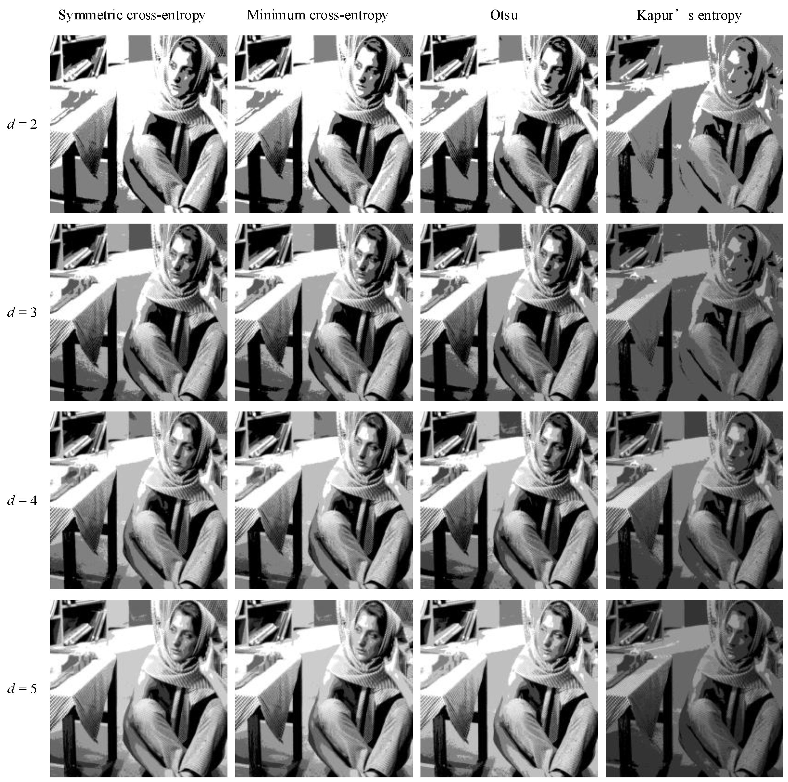
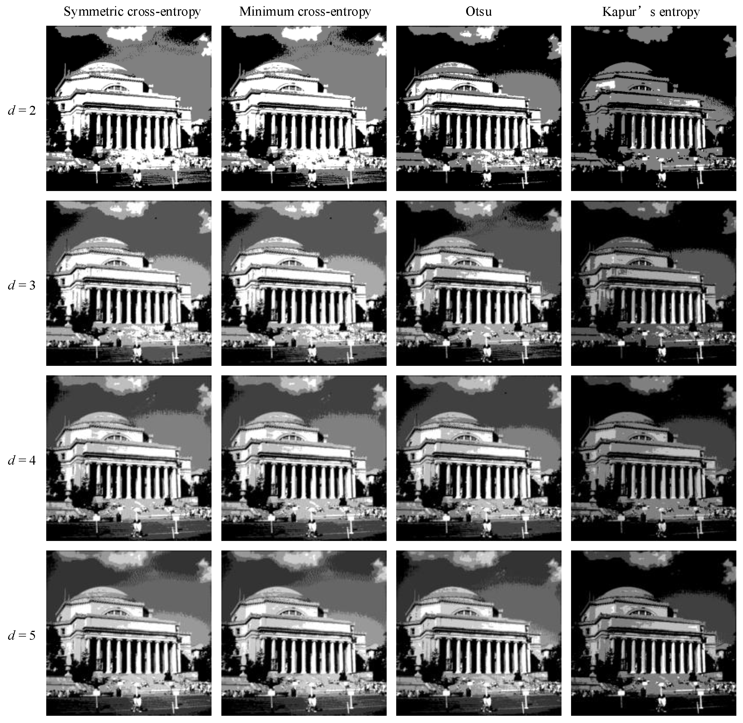
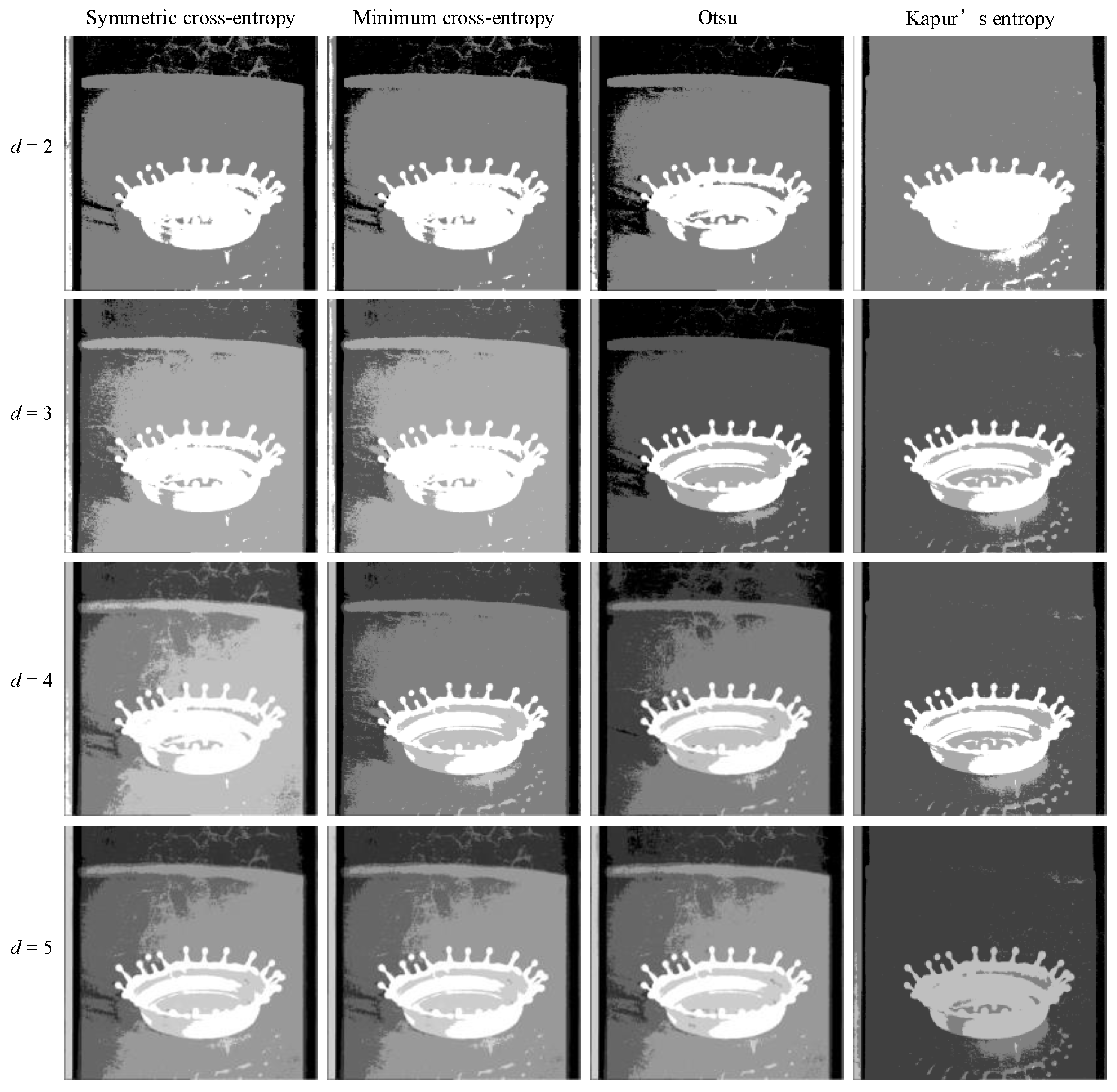
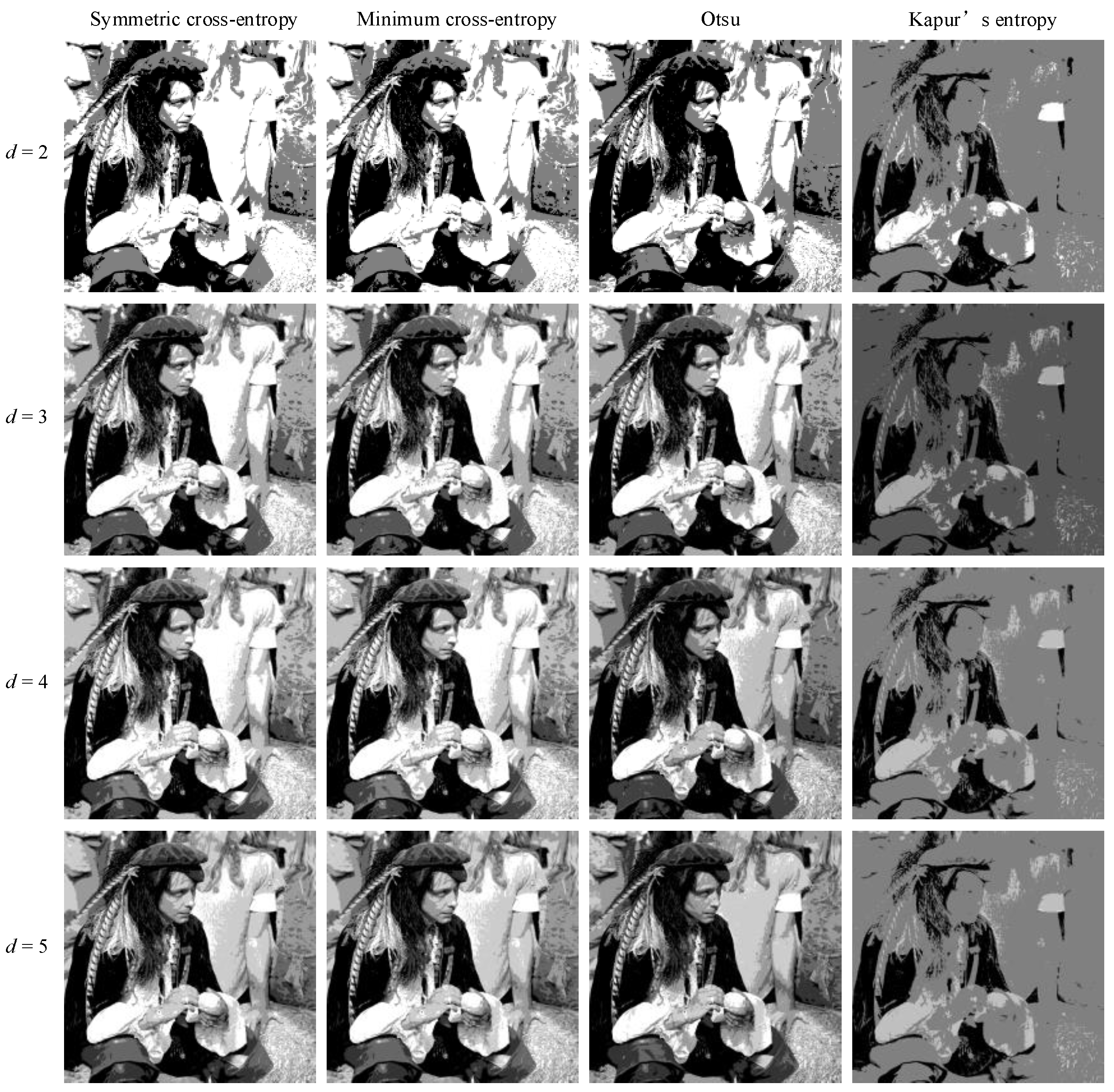
6.1. Threshold Segmentation Experiment for the Segmentation Criteria
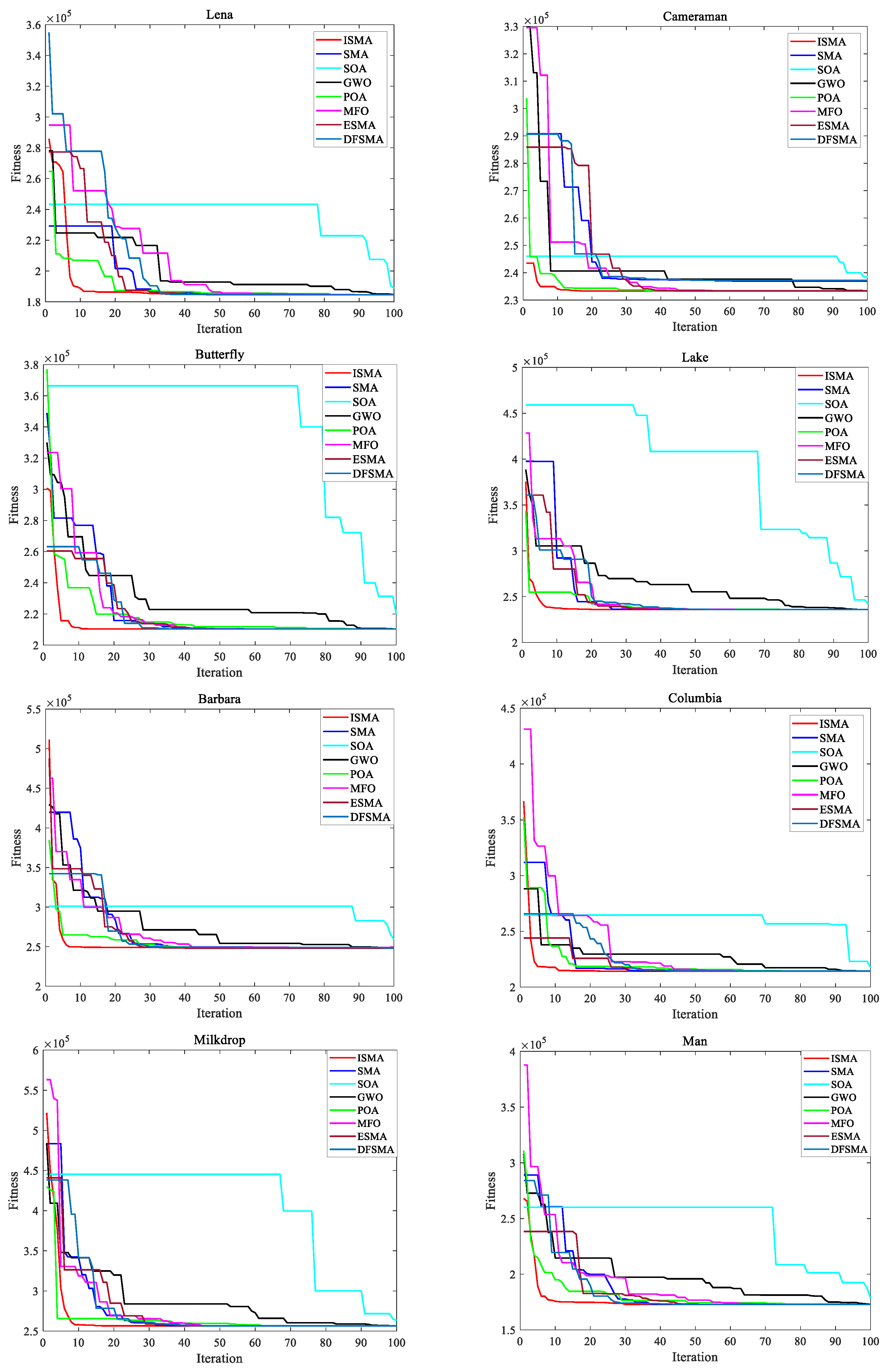
6.2. Threshold Segmentation Experiment of MAs
7. Conclusions
Author Contributions
Funding
Institutional Review Board Statement
Informed Consent Statement
Data Availability Statement
Conflicts of Interest
References
- Hosny, K.M.; Khalid, A.M.; Hamza, H.M.; Mirjalili, S. Multilevel segmentation of 2D and volumetric medical images using hybrid Coronavirus Optimization Algorithm. Comput. Biol. Med. 2022, 150, 106003. [Google Scholar] [CrossRef] [PubMed]
- Chen, S.; Qiu, C.; Yang, W.; Zhang, Z. Combining edge guidance and feature pyramid for medical image segmentation. Biomed. Signal Process. Control 2022, 78, 103960. [Google Scholar] [CrossRef]
- Li, Y.; Xuan, Y.; Zhao, Q. Remote sensing image segmentation by combining manifold projection and persistent homology. Measurement 2022, 198, 111414. [Google Scholar] [CrossRef]
- Zhao, S.; Wang, P.; Heidari, A.A.; Chen, H.; He, W.; Xu, S. Performance optimization of salp swarm algorithm for multi-threshold image segmentation: Comprehensive study of breast cancer microscopy. Comput. Biol. Med. 2021, 139, 105015. [Google Scholar] [CrossRef]
- Wang, G.; Guo, S.; Han, L.; Cekderi, A.B. Two-dimensional reciprocal cross entropy multi-threshold combined with improved firefly algorithm for lung parenchyma segmentation of COVID-19 CT image. Biomed. Signal Process. Control 2022, 78, 103933. [Google Scholar] [CrossRef]
- Yu, H.; Song, J.; Chen, C.; Heidari, A.A.; Liu, J.; Chen, H.; Zaguia, A.; Mafarja, M. Image segmentation of Leaf Spot Diseases on Maize using multi-stage Cauchy-enabled grey wolf algorithm. Eng. Appl. Artif. Intell. 2022, 109, 104653. [Google Scholar] [CrossRef]
- Shitharth, S.; Manoharan, H.; Alshareef, A.M.; Yafoz, A.; Alkhiri, H.; Mirza, O.M. Hyper spectral image classifications for monitoring harvests in agriculture using fly optimization algorithm. Comput. Electr. Eng. 2022, 103, 108400. [Google Scholar]
- Rahaman, J.; Sing, M. An efficient multilevel thresholding based satellite image segmentation approach using a new adaptive cuckoo search algorithm. Expert Syst. Appl. 2021, 174, 114633. [Google Scholar] [CrossRef]
- Jumiawi, W.A.H.; El-Zaart, A. Improvement in the Between-Class Variance Based on Lognormal Distribution for Accurate Image Segmentation. Entropy 2022, 24, 1204. [Google Scholar] [CrossRef]
- Liu, Q.; Li, N.; Jia, H.; Qi, Q.; Abualigah, L. Modified Remora Optimization Algorithm for Global Optimization and Multilevel Thresholding Image Segmentation. Mathematics 2022, 10, 1014. [Google Scholar] [CrossRef]
- Giacomini, M.; Perotto, S. Anisotropic mesh adaptation for region-based segmentation accounting for image spatial information. Comput. Math. Appl. 2022, 121, 17. [Google Scholar] [CrossRef]
- Xie, L.; Chen, Z.; Sheng, X.; Zeng, Q.; Huang, J.; Wen, C.; Wen, L.; Xie, G.; Feng, Y. Semi-supervised region-connectivity-based cerebrovascular segmentation for time-of-flight magnetic resonance angiography image. Comput. Biol. Med. 2022, 149, 105972. [Google Scholar] [CrossRef]
- Wu, C.; Wang, Z. A modified fuzzy dual-local information c-mean clustering algorithm using quadratic surface as prototype for image segmentation. Expert Syst. Appl. 2022, 201, 117019. [Google Scholar] [CrossRef]
- Chen, L.; Zhao, Y.P.; Zhang, C. Efficient kernel fuzzy clustering via random Fourier superpixel and graph prior for color image segmentation. Eng. Appl. Artif. Intell. 2022, 116, 105335. [Google Scholar] [CrossRef]
- Wu, B.; Zhou, J.; Ji, X.; Yin, Y.; Shen, X. An ameliorated teaching–learning-based optimization algorithm based study of image segmentation for multilevel thresholding using Kapur’s entropy and Otsu’s between class variance. Inf. Sci. 2020, 533, 72–107. [Google Scholar] [CrossRef]
- Song, S.; Jia, H.; Ma, J. A Chaotic Electromagnetic Field Optimization Algorithm Based on Fuzzy Entropy for Multilevel Thresholding Color Image Segmentation. Entropy 2019, 21, 398. [Google Scholar] [CrossRef] [Green Version]
- Lin, S.; Jia, H.; Abualigah, L.; Altalhi, M. Enhanced Slime Mould Algorithm for Multilevel Thresholding Image Segmentation Using Entropy Measures. Entropy 2021, 23, 1700. [Google Scholar] [CrossRef]
- Dhiman, G.; Kumar, V. Seagull optimization algorithm: Theory and its applications for large-scale industrial engineering problems. Knowl. -Based Syst. 2019, 165, 169–196. [Google Scholar] [CrossRef]
- Rezaei, F.; Safavi, H.R.; Abd Elaziz, M.; Abualigah, L.; Mirjalili, S.; Gandomi, A.H. Diversity-Based Evolutionary Population Dynamics: A New Operator for Grey Wolf Optimizer. Processes 2022, 10, 2615. [Google Scholar] [CrossRef]
- Xue, J.; Shen, B. A novel swarm intelligence optimization approach: Sparrow search algorithm. Syst. Sci. Control Eng. 2020, 8, 22–34. [Google Scholar] [CrossRef]
- Anand, R.; Samiaappan, S.; Veni, S.; Worch, E.; Zhou, M. Airborne Hyperspectral Imagery for Band Selection Using Moth–Flame Metaheuristic Optimization. J. Imaging 2022, 8, 126. [Google Scholar] [CrossRef] [PubMed]
- Trojovský, P.; Dehghani, M. Pelican Optimization Algorithm: A Novel Nature-Inspired Algorithm for Engineering Applications. Sensors 2022, 22, 855. [Google Scholar] [CrossRef] [PubMed]
- Abd Elaziz, M.; Ewees, A.A.; Oliva, D. Hyper-heuristic method for multilevel thresholding image segmentation. Expert Syst. Appl. 2020, 146, 113201. [Google Scholar] [CrossRef]
- Lang, C.; Jia, H. Kapur’s Entropy for Color Image Segmentation Based on a Hybrid Whale Optimization Algorithm. Entropy 2019, 21, 318. [Google Scholar] [CrossRef] [Green Version]
- Xiaobing, Y.; Xuejing, W. Ensemble grey wolf Optimizer and its application for image segmentation. Expert Syst. Appl. 2022, 209, 118267. [Google Scholar]
- Zhao, D.; Liu, L.; Yu, F.; Heidari, A.A.; Wang, M.; Liang, G.; Muhammad, K.; Chen, H. Chaotic random spare ant colony optimization for multi-threshold image segmentation of 2D Kapur entropy. Knowl. -Based Syst. 2021, 216, 106510. [Google Scholar] [CrossRef]
- Houssein, E.H.; Helmy, B.E.D.; Oliva, D.; Elngar, A.A.; Shaban, H. A novel Black Widow Optimization algorithm for multilevel thresholding image segmentation. Expert Syst. Appl. 2021, 167, 114159. [Google Scholar] [CrossRef]
- Chen, Y.; Wang, M.; Heidari, A.A.; Shi, B.; Hu, Z.; Zhang, Q.; Chen, H.; Mafarja, M.; Turabieh, H. Multi-threshold image segmentation using a multi-strategy shuffled frog leaping algorithm. Expert Syst. Appl. 2022, 194, 116511. [Google Scholar] [CrossRef]
- Li, S.; Chen, H.; Wang, M.; Heidari, A.A.; Mirjalili, S. Slime mould algorithm: A new method for stochastic optimization. Future Gener. Comput. Syst. 2020, 111, 300–323. [Google Scholar]
- Örnek, B.N.; Aydemir, S.B.; Düzenli, T.; Özak, B. A novel version of slime mould algorithm for global optimization and real world engineering problems: Enhanced slime mould algorithm. Math. Comput. Simul. 2022, 198, 253–288. [Google Scholar] [CrossRef]
- Hu, J.; Gui, W.; Heidari, A.A.; Cai, Z.; Liang, G.; Chen, H.; Pan, Z. Dispersed foraging slime mould algorithm: Continuous and binary variants for global optimization and wrapper-based feature selection. Knowl. -Based Syst. 2022, 237, 107761. [Google Scholar] [CrossRef]
- Chen, H.; Li, W.; Yang, X. A whale optimization algorithm with chaos mechanism based on quasi-opposition for global optimization problems. Expert Syst. Appl. 2020, 158, 113612. [Google Scholar] [CrossRef]
- Esparza, E.R.; Calzada, L.A.Z.; Oliva, D.; Heidari, A.A.; Zaldivar, D.; Cisneros, M.P.; Foong, L.K. An efficient harris hawks-inspired image segmentation method. Expert Syst. Appl. 2020, 155, 113428. [Google Scholar] [CrossRef]
- Gill, H.S.; Khehra, B.S.; Singh, A.; Kaur, L. Teaching-learning-based optimization algorithm to minimize cross entropy for Selecting multilevel threshold values. Egypt. Inform. J. 2018, 20, 11–25. [Google Scholar] [CrossRef]
- Wang, M.; Wang, W.; Li, L.; Zhou, Z. Optimizing Multiple Entropy Thresholding by the Chaotic Combination Strategy Sparrow Search Algorithm for Aggregate Image Segmentation. Entropy 2022, 24, 1788. [Google Scholar] [CrossRef] [PubMed]


| No | Name | Range | D | fmin | Type |
|---|---|---|---|---|---|
| F1 | Sphere | [−100, 100] | 30 | 0 | UM |
| F2 | Schwefel 2.22 | [−10, 10] | 30 | 0 | UM |
| F3 | Schwefel 1.2 | [−100, 100] | 30 | 0 | UM |
| F4 | Schwefel 2.21 | [−100, 100] | 30 | 0 | UM |
| F5 | Rosenbrock | [−30, 30] | 30 | 0 | UM |
| F6 | Step | [−100, 100] | 30 | 0 | UM |
| F7 | Quartic | [−1.28, 1.28] | 30 | 0 | UM |
| F8 | Schwefel | [−500, 500] | 30 | −12,569.487 | MM |
| F9 | Rastrigin | [−5.12, 5.12] | 30 | 0 | MM |
| F10 | Ackley | [−32, 32] | 30 | 0 | MM |
| F11 | Griewank | [−600, 600] | 30 | 0 | MM |
| F12 | Penalized | [−50, 50] | 30 | 0 | MM |
| F13 | Penalized 2 | [−50, 50] | 30 | 0 | MM |
| F14 | Foxholes | [−65.536, 65.536] | 2 | 0.998004 | MM |
| Algorithm | Parameters |
|---|---|
| ISMA | Z = 0.03 |
| SMA | Z = 0.03 |
| SOA | FC = 2, u = 1, v = 1 |
| MFO | b = 1, = 0.001, g ∈ [0, 30], C ∈ [0, 100] |
| GWO | a ∈ [2, 0] |
| POA | I = 2, R = 0.2 |
| ESMA | Z = 0.03 |
| DFSMA | Z = 0.03 |
| Function | ISMA | SMA | SOA | MFO | POA | GWO | ESMA | DFSMA |
|---|---|---|---|---|---|---|---|---|
| F1 | 0.000 | 1.500 × 10−323 | 8.496 × 10⁻¹² | 1.341 × 10³ | 1.525 × 10−103 | 1.619 × 10⁻²⁸ | 5.106 × 10−297 | 2.320 × 10−292 |
| F2 | 0.000 | 6.348 × 10−147 | 1.590 × 10⁻⁸ | 3.685 × 10 | 6.001 × 10−52 | 9.760 × 10⁻¹⁷ | 3.758 × 10−168 | 9.280 × 10−153 |
| F3 | 0.000 | 1.446 × 10−313 | 1.258 × 10⁻⁴ | 2.109 × 10⁴ | 3.735 × 10−100 | 7.918 × 10⁻⁶ | 2.970 × 10−296 | 5.900 × 10−323 |
| F4 | 0.000 | 1.007 × 10−148 | 1.758 × 10⁻² | 6.794 × 10 | 2.443 × 10−51 | 6.649 × 10⁻⁷ | 4.231 × 10−141 | 1.983 × 10−160 |
| F5 | 2.550 | 1.207 × 101 | 2.822 × 10 | 2.688 × 10⁶ | 2.810 × 10 | 2.682 × 10 | 5.415 | 3.262 |
| F6 | 4.239 × 10⁻⁴ | 7.500 × 10⁻³ | 3.306 | 1.680 × 10³ | 2.829 | 7.552 × 10⁻¹ | 5.803 × 10⁻³ | 5.431 × 10⁻³ |
| F7 | 1.211 × 10⁻⁴ | 1.805 × 10⁻⁴ | 2.631 × 10⁻³ | 5.766 | 2.363 × 10⁻⁴ | 1.657 × 10⁻³ | 1.950 × 10⁻⁴ | 1.685 × 10⁻⁴ |
| F8 | −1.257 × 10⁴ | −1.257 × 10⁴ | −4.861 × 10³ | 9.933 × 10² | −7.642 × 10³ | −5.930 × 10³ | −1.256 × 10⁴ | −1.256 × 10⁴ |
| F9 | 0.000 | 0.000 | 1.297 | 1.714 × 10² | 0.000 | 4.815 | 0.000 | 0.000 |
| F10 | 8.882 × 10⁻¹⁶ | 8.882 × 10⁻¹⁶ | 1.996 × 10 | 1.448 × 10 | 3.257 × 10⁻¹⁵ | 9.456 × 10⁻¹⁴ | 8.882 × 10⁻¹⁶ | 8.882 × 10⁻¹⁶ |
| F11 | 0.000 | 0.000 | 2.989 × 10⁻² | 1.591 × 10 | 0.000 | 4.596 × 10⁻³ | 0.000 | 0.000 |
| F12 | 3.098 × 10⁻⁴ | 5.500 × 10⁻³ | 3.439 × 10⁻¹ | 8.534 × 10⁶ | 1.926 × 10⁻¹ | 5.065 × 10⁻² | 5.237 × 10⁻³ | 4.620 × 10⁻³ |
| F13 | 1.700 × 10⁻³ | 1.240 × 10⁻² | 2.057 | 2.381 × 10² | 2.589 | 5.603 × 10⁻¹ | 6.689 × 10⁻³ | 6.933 × 10⁻³ |
| F14 | 9.980 × 10⁻¹ | 1.013 | 2.150 | 1.823 | 1.823 | 4.655 | 9.981 × 10⁻¹ | 9.981 × 10⁻¹ |
| Function | ISMA | SMA | SOA | MFO | POA | GWO | ESMA | DFSMA |
|---|---|---|---|---|---|---|---|---|
| F1 | 0.000 | 0.000 | 1.787 × 10⁻¹¹ | 4.340 × 10³ | 7.328 × 10−103 | 2.412 × 10⁻²⁷ | 0.000 | 0.000 |
| F2 | 0.000 | 3.477 × 10−146 | 1.791 × 10⁻⁸ | 2.778 × 10 | 2.117 × 10−51 | 5.044 × 10⁻¹⁷ | 1.776 × 10−156 | 5.082 × 10−152 |
| F3 | 0.000 | 0.000 | 5.100 × 10⁻⁴ | 9.875 × 10³ | 1.932 × 10−99 | 1.388 × 10⁻⁵ | 0.000 | 0.000 |
| F4 | 0.000 | 5.518 × 10−148 | 7.711 × 10⁻² | 6.246 | 1.187 × 10−50 | 5.612 × 10⁻⁷ | 2.317 × 10−140 | 1.086 × 10−159 |
| F5 | 5.023 | 1.354 × 1001 | 2.883 × 10 | 2.004 × 10² | 8.098 × 10⁻¹ | 2.711 × 10 | 9.366 | 7.662 |
| F6 | 7.757 × 10⁻⁴ | 3.100 × 10⁻³ | 4.505 × 10⁻¹ | 3.795 × 10³ | 6.616 × 10⁻¹ | 3.078 × 10⁻¹ | 3.336 × 10⁻³ | 2.451 × 10⁻³ |
| F7 | 1.110 × 10⁻⁴ | 1.431 × 10⁻⁴ | 2.043 × 10⁻³ | 1.143 × 101 | 1.797 × 10−04 | 8.672 × 10⁻⁴ | 1.527 × 10⁻⁴ | 1.715 × 10⁻⁴ |
| F8 | 3.087 × 10⁻¹ | 1.575 × 101 | 4.834 × 10² | 3.985 × 10³ | 7.531 × 1002 | 8.413 × 10² | 4.327 × 10⁻¹ | 3.812 × 10⁻¹ |
| F9 | 0.000 | 0.000 | 2.348 | 4.479 × 101 | 0.000 | 7.065 | 0.000 | 0.000 |
| F10 | 0.000 | 0.000 | 1.540 × 10⁻³ | 6.998 | 1.703 × 10⁻¹⁵ | 1.410 × 10⁻¹⁴ | 0.000 | 0.000 |
| F11 | 0.000 | 0.000 | 5.084 × 10⁻² | 3.407 × 101 | 0.000 | 9.000 × 10⁻³ | 0.000 | 0.000 |
| F12 | 6.516 × 10⁻⁴ | 5.000 × 10⁻³ | 1.016 × 10⁻¹ | 2.492 × 10² | 7.090 × 10−02 | 1.918 × 10⁻² | 7.366 × 10⁻³ | 6.237 × 10⁻³ |
| F13 | 2.100 × 10⁻³ | 1.230 × 10⁻² | 1.449 × 10⁻¹ | 8.193 × 10² | 4.345 × 10⁻¹ | 2.567 × 10⁻¹ | 8.739 × 10⁻³ | 8.789 × 10⁻³ |
| F14 | 3.593 × 10⁻¹³ | 6.655 × 10⁻² | 1.891 | 1.399 | 1.399 | 4.146 | 5.955 × 10⁻¹³ | 4.627 × 10⁻¹³ |
| Function | ISMA | SMA | SOA | MFO | POA | GWO | ESMA | DFSMA |
|---|---|---|---|---|---|---|---|---|
| F1 | 3.292 × 10⁻¹ | 3.207 × 10⁻¹ | 3.090 × 10⁻¹ | 2.812 × 10⁻¹ | 1.963 × 10⁻¹ | 5.205 × 10⁻¹ | 3.533 × 10⁻¹ | 3.450 × 10⁻¹ |
| F2 | 3.442 × 10⁻² | 3.424 × 10⁻¹ | 3.541 × 10⁻¹ | 3.331 × 10⁻¹ | 2.219 × 10⁻¹ | 5.747 × 10⁻¹ | 3.755 × 10⁻¹ | 3.739 × 10⁻¹ |
| F3 | 4.387 × 10⁻¹ | 4.348 × 10⁻¹ | 4.248 × 10⁻¹ | 3.998 × 10⁻¹ | 4.523 × 10⁻¹ | 6.052 × 10⁻¹ | 4.765 × 10⁻¹ | 4.739 × 10⁻¹ |
| F4 | 3.334 × 10⁻¹ | 3.262 × 10⁻¹ | 2.783 × 10⁻¹ | 2.425 × 10⁻¹ | 1.583 × 10⁻¹ | 4.419 × 10⁻¹ | 3.593 × 10⁻¹ | 3.354 × 10⁻¹ |
| F5 | 3.522 × 10⁻¹ | 3.433 × 10⁻¹ | 2.885 × 10⁻¹ | 2.510 × 10⁻¹ | 1.822 × 10⁻¹ | 4.630 × 10⁻¹ | 3.854 × 10⁻¹ | 3.702 × 10⁻¹ |
| F6 | 3.388 × 10⁻¹ | 3.290 × 10⁻¹ | 2.886 × 10⁻¹ | 2.597 × 10⁻¹ | 1.862 × 10⁻¹ | 4.395 × 10⁻¹ | 3.685 × 10⁻¹ | 3.539 × 10⁻¹ |
| F7 | 3.892 × 10⁻¹ | 3.812 × 10⁻¹ | 3.171 × 10⁻¹ | 2.853 × 10⁻¹ | 2.595 × 10⁻¹ | 4.876 × 10⁻¹ | 4.282 × 10⁻¹ | 1.071 × 10⁻¹ |
| F8 | 3.535 × 10⁻¹ | 3.383 × 10⁻¹ | 3.408 × 10⁻¹ | 2.884 × 10⁻¹ | 2.670 × 10⁻¹ | 4.838 × 10⁻¹ | 3.938 × 10⁻¹ | 3.638 × 10⁻¹ |
| F9 | 3.325 × 10⁻¹ | 3.233 × 10⁻¹ | 2.813 × 10⁻¹ | 2.532 × 10⁻¹ | 2.013 × 10⁻¹ | 4.588 × 10⁻¹ | 3.721 × 10⁻¹ | 3.422 × 10⁻¹ |
| F10 | 3.396 × 10⁻¹ | 3.255 × 10⁻¹ | 2.830 × 10⁻¹ | 2.560 × 10⁻¹ | 1.781 × 10⁻¹ | 4.495 × 10⁻¹ | 3.654 × 10⁻¹ | 3.598 × 10⁻¹ |
| F11 | 3.571 × 10⁻¹ | 3.347 × 10⁻¹ | 3.008 × 10⁻¹ | 2.652 × 10⁻¹ | 2.005 × 10⁻¹ | 4.640 × 10⁻¹ | 3.933 × 10⁻¹ | 3.654 × 10⁵ |
| F12 | 5.140 × 10⁻¹ | 4.973 × 10⁻¹ | 4.824 × 10⁻¹ | 4.385 × 10⁻¹ | 5.666 × 10⁻¹ | 6.634 × 10⁻¹ | 5.535 × 10⁻¹ | 5.449 × 10⁻¹ |
| F13 | 5.017 × 10⁻¹ | 4.978 × 10⁻¹ | 4.806 × 10⁻¹ | 4.500 × 10⁻¹ | 5.501 × 10⁻¹ | 6.495 × 10⁻¹ | 5.727 × 10⁻¹ | 5.220 × 10⁻¹ |
| F14 | 5.090 × 10⁻¹ | 5.042 × 10⁻¹ | 4.681 × 10⁻¹ | 4.547 × 10⁻¹ | 8.880 × 10⁻¹ | 4.741 × 10⁻¹ | 5.748 × 10⁻¹ | 5.382 × 10⁻¹ |
| Images | d | Symmetric Cross-Entropy | Minimum Cross-Entropy | Otsu | Kapur’s Entropy | ||||||||
|---|---|---|---|---|---|---|---|---|---|---|---|---|---|
| PSNR | SSIM | FSIM | PSNR | SSIM | FSIM | PSNR | SSIM | FSIM | PSNR | SSIM | FSIM | ||
| Lena | 2 | 13.2058 | 0.4969 | 0.6978 | 12.2497 | 0.4949 | 0.6976 | 12.0066 | 0.4723 | 0.6897 | 7.7212 | 0.1290 | 0.5866 |
| 3 | 15.7899 | 0.5628 | 0.7660 | 15.6702 | 0.5607 | 0.7654 | 15.6612 | 0.5362 | 0.7542 | 13.3143 | 0.5223 | 0.6812 | |
| 4 | 16.5512 | 0.5776 | 0.8029 | 16.2183 | 0.5632 | 0.7956 | 16.2183 | 0.5580 | 0.7954 | 15.4882 | 0.5661 | 0.6985 | |
| 5 | 17.0899 | 0.6802 | 0.8305 | 16.7296 | 0.6115 | 0.8305 | 16.9276 | 0.5814 | 0.8289 | 17.0600 | 0.5998 | 0.7196 | |
| Cameraman | 2 | 12.0475 | 0.5555 | 0.7662 | 11.5227 | 0.5562 | 0.7554 | 11.5288 | 0.5551 | 0.7549 | 11.3573 | 0.4941 | 0.6504 |
| 3 | 12.8391 | 0.5982 | 0.8097 | 11.5551 | 0.5980 | 0.8074 | 11.5670 | 0.5739 | 0.7910 | 12.4609 | 0.5567 | 0.6530 | |
| 4 | 16.1448 | 0.6089 | 0.8344 | 12.7883 | 0.6089 | 0.8344 | 12.7883 | 0.5984 | 0.8192 | 12.9698 | 0.5646 | 0.6742 | |
| 5 | 16.6072 | 0.6384 | 0.8584 | 14.8859 | 0.6276 | 0.8447 | 15.7175 | 0.6175 | 0.8576 | 16.4663 | 0.5876 | 0.6746 | |
| Butterfly | 2 | 13.2788 | 0.5266 | 0.7363 | 13.1412 | 0.5266 | 0.7330 | 13.1412 | 0.4730 | 0.7363 | 11.7625 | 0.3130 | 0.7101 |
| 3 | 15.5515 | 0.5759 | 0.7914 | 14.9690 | 0.5759 | 0.7338 | 14.9690 | 0.5603 | 0.7738 | 14.0402 | 0.4095 | 0.7524 | |
| 4 | 16.4086 | 0.6147 | 0.8153 | 15.9752 | 0.6147 | 0.8079 | 16.0354 | 0.6183 | 0.8153 | 16.0276 | 0.6435 | 0.7821 | |
| 5 | 16.6381 | 0.6474 | 0.8281 | 16.0354 | 0.6327 | 0.8143 | 16.1095 | 0.7103 | 0.8182 | 16.5343 | 0.6478 | 0.8136 | |
| Lake | 2 | 13.1104 | 0.5017 | 0.7314 | 12.9005 | 0.5002 | 0.7313 | 12.9179 | 0.4781 | 0.7313 | 13.3854 | 0.4398 | 0.6234 |
| 3 | 16.1352 | 0.5589 | 0.7908 | 14.0479 | 0.5589 | 0.7835 | 14.0479 | 0.5180 | 0.7835 | 16.2402 | 0.5150 | 0.6565 | |
| 4 | 18.0386 | 0.6572 | 0.8391 | 18.0386 | 0.6071 | 0.8257 | 17.3537 | 0.5589 | 0.8257 | 15.8882 | 0.5346 | 0.6918 | |
| 5 | 18.6824 | 0.6948 | 0.8623 | 18.4376 | 0.6542 | 0.8412 | 18.2994 | 0.6071 | 0.8360 | 15.8486 | 0.6575 | 0.7275 | |
| Barbara | 2 | 14.7227 | 0.4756 | 0.7278 | 12.6622 | 0.4756 | 0.7278 | 13.1800 | 0.4631 | 0.7261 | 14.7227 | 0.4663 | 0.6874 |
| 3 | 16.3754 | 0.5432 | 0.7943 | 16.3754 | 0.5432 | 0.7942 | 15.6470 | 0.5347 | 0.7943 | 15.8715 | 0.4933 | 0.7339 | |
| 4 | 16.9175 | 0.6023 | 0.8304 | 16.8855 | 0.6023 | 0.8301 | 16.6012 | 0.5770 | 0.8104 | 15.9885 | 0.5687 | 0.8294 | |
| 5 | 17.9234 | 0.6553 | 0.8512 | 17.0108 | 0.6545 | 0.8500 | 17.1495 | 0.6064 | 0.8289 | 17.9234 | 0.5913 | 0.8441 | |
| Columbia | 2 | 13.8785 | 0.3900 | 0.7056 | 11.2266 | 0.3900 | 0.6707 | 12.7799 | 0.3157 | 0.6707 | 13.8758 | 0.2524 | 0.7020 |
| 3 | 15.3874 | 0.5372 | 0.7812 | 13.0064 | 0.5372 | 0.7338 | 13.0064 | 0.4605 | 0.7618 | 15.3316 | 0.3551 | 0.7812 | |
| 4 | 16.2809 | 0.6030 | 0.8030 | 14.7853 | 0.5993 | 0.7827 | 15.2117 | 0.6014 | 0.8000 | 15.9069 | 0.3952 | 0.8030 | |
| 5 | 16.7908 | 0.6269 | 0.8200 | 15.2117 | 0.6250 | 0.8086 | 15.9069 | 0.6250 | 0.8042 | 16.0853 | 0.3905 | 0.8042 | |
| Milkdrop | 2 | 15.8750 | 0.6458 | 0.7313 | 12.9792 | 0.5851 | 0.7242 | 15.8750 | 0.5552 | 0.7266 | 13.3613 | 0.5906 | 0.7075 |
| 3 | 18.4471 | 0.6644 | 0.7845 | 15.4290 | 0.6063 | 0.7511 | 17.4501 | 0.5968 | 0.7544 | 18.4471 | 0.5956 | 0.7371 | |
| 4 | 19.3641 | 0.6849 | 0.8207 | 17.2172 | 0.6739 | 0.7627 | 18.3448 | 0.6285 | 0.7985 | 19.2545 | 0.6035 | 0.7525 | |
| 5 | 19.7948 | 0.6880 | 0.8309 | 19.2545 | 0.6849 | 0.8303 | 19.3641 | 0.6621 | 0.8262 | 19.3641 | 0.6727 | 0.7544 | |
| Man | 2 | 14.6403 | 0.4300 | 0.6925 | 11.0410 | 0.3867 | 0.6845 | 12.2389 | 0.3681 | 0.6845 | 14.6403 | 0.4033 | 0.6144 |
| 3 | 16.4136 | 0.4763 | 0.7664 | 13.7597 | 0.4708 | 0.7657 | 14.1385 | 0.4634 | 0.7636 | 16.4136 | 0.4313 | 0.6393 | |
| 4 | 17.3328 | 0.5114 | 0.8147 | 13.9758 | 0.5114 | 0.7959 | 16.5070 | 0.5053 | 0.7959 | 16.5070 | 0.4696 | 0.6393 | |
| 5 | 17.7032 | 0.5753 | 0.8453 | 16.1596 | 0.5570 | 0.8362 | 17.3328 | 0.5517 | 0.8362 | 17.7032 | 0.4696 | 0.6545 | |
| Images | d | Symmetric Cross-Entropy | Minimum Cross-Entropy | Otsu | Kapur’s Entropy |
|---|---|---|---|---|---|
| Lena | 2 | 82 140 | 82 142 | 92 151 | 163 220 |
| 3 | 73 120 166 | 74 121 167 | 80 126 170 | 59 164 220 | |
| 4 | 71 109 140 175 | 70 109 139 175 | 74 113 145 180 | 57 60 164 221 | |
| 5 | 62 88 118 147 180 | 62 88 117 146 180 | 73 109 136 160 188 | 58 162 180 217 236 | |
| Cameraman | 2 | 54 137 | 52 137 | 70 144 | 19 193 |
| 3 | 31 94 144 | 30 84 145 | 57 116 154 | 18 21 194 | |
| 4 | 30 77 124 157 | 29 76 125 157 | 40 93 140 170 | 1 17 20 193 | |
| 5 | 28 71 112 144 172 | 28 71 113 145 172 | 36 83 122 149 173 | 1 16 19 21 194 | |
| Butterfly | 2 | 76 138 | 76 138 | 85 148 | 114 206 |
| 3 | 67 108 158 | 67 107 159 | 75 120 170 | 97 125 207 | |
| 4 | 62 92 128 172 | 62 93 128 172 | 66 99 135 177 | 57 102 126 208 | |
| 5 | 59 82 107 137 177 | 57 81 104 135 176 | 36 83 122 149 173 | 57 101 126 205 235 | |
| Lake | 2 | 74 143 | 75 142 | 86 155 | 73 228 |
| 3 | 65 107 163 | 64 162 107 | 80 141 194 | 62 86 228 | |
| 4 | 60 93 145 196 | 60 94 145 195 | 68 111 158 199 | 9 62 86 228 | |
| 5 | 53 77 112 155 197 | 55 80 116 160 199 | 60 91 128 166 200 | 10 29 72 89 228 | |
| Barbara | 2 | 74 138 | 74 139 | 82 147 | 54 174 |
| 3 | 67 119 170 | 68 119 171 | 75 127 176 | 55 169 222 | |
| 4 | 56 93 132 176 | 56 92 133 177 | 66 106 142 182 | 54 128 174 223 | |
| 5 | 47 76 108 141 181 | 48 76 108 142 180 | 57 88 118 148 184 | 54 129 174 218 241 | |
| Columbia | 2 | 59 110 | 60 109 | 75 130 | 93 177 |
| 3 | 50 83 130 | 50 83 129 | 61 102 152 | 77 147 211 | |
| 4 | 45 71 105 148 | 45 71 104 148 | 50 79 115 159 | 74 102 162 218 | |
| 5 | 39 59 81 111 151 | 40 60 82 113 155 | 48 74 103 135 171 | 73 101 152 190 234 | |
| Milkdrop | 2 | 65 140 | 68 142 | 76 154 | 120 173 |
| 3 | 35 83 150 | 33 81 145 | 72 127 188 | 16 120 173 | |
| 4 | 33 68 99 154 | 33 80 127 185 | 51 90 132 190 | 1 16 121 173 | |
| 5 | 33 68 96 131 187 | 31 67 95 132 187 | 37 70 97 134 191 | 1 16 118 154 241 | |
| Man | 2 | 75 130 | 76 130 | 87 142 | 54 181 |
| 3 | 67 109 152 | 66 108 152 | 71 114 156 | 55 176 224 | |
| 4 | 60 90 122 158 | 60 91 122 158 | 68 107 141 173 | 50 59 176 224 | |
| 5 | 59 85 113 143 173 | 59 85 113 142 173 | 63 94 123 151 182 | 1 50 58 176 225 |
| Images | d | ISMA | GWO | SOA | SMA | POA | MFO | ESMA | DFSMA |
|---|---|---|---|---|---|---|---|---|---|
| Lena | 2 | 13.2058 | 13.2058 | 13.2058 | 13.2058 | 12.0066 | 12.0066 | 12.0066 | 12.0066 |
| 3 | 15.7899 | 15.7038 | 15.5352 | 15.7810 | 15.5612 | 15.5612 | 15.6512 | 15.6512 | |
| 4 | 16.5512 | 16.4458 | 16.4631 | 16.5291 | 16.2183 | 16.2183 | 16.2183 | 16.2183 | |
| 5 | 17.0899 | 16.7296 | 16.7296 | 16.7457 | 16.6878 | 16.7296 | 16.7296 | 16.7296 | |
| Cameraman | 2 | 12.0475 | 11.9735 | 11.9735 | 12.0475 | 11.5288 | 11.5288 | 11.5288 | 11.5288 |
| 3 | 12.8391 | 12.7378 | 12.6314 | 12.7460 | 11.5670 | 11.5670 | 11.5670 | 11.5670 | |
| 4 | 16.1448 | 16.1086 | 12.8239 | 16.1432 | 12.7883 | 12.7883 | 12.7883 | 12.7883 | |
| 5 | 16.6072 | 16.3075 | 13.2107 | 16.4663 | 15.7326 | 15.7175 | 14.7133 | 15.4820 | |
| Butterfly | 2 | 13.2788 | 13.2280 | 13.1618 | 13.2280 | 13.1412 | 13.1412 | 13.1412 | 13.1412 |
| 3 | 15.5515 | 15.5453 | 15.5163 | 15.4508 | 14.9690 | 14.9690 | 14.9690 | 14.9690 | |
| 4 | 16.4086 | 16.2999 | 16.2608 | 16.3081 | 16.0354 | 16.0354 | 15.9752 | 16.0354 | |
| 5 | 16.6381 | 16.3552 | 16.3139 | 16.4275 | 16.1095 | 16.1095 | 16.0354 | 16.1095 | |
| Lake | 2 | 13.1104 | 13.1104 | 13.0815 | 13.1104 | 12.9179 | 12.9179 | 12.9179 | 12.9179 |
| 3 | 16.1352 | 16.0206 | 15.9760 | 16.0328 | 14.0479 | 14.0249 | 14.0479 | 14.0479 | |
| 4 | 18.0386 | 18.0386 | 15.1716 | 18.0386 | 18.0386 | 18.0386 | 18.0386 | 18.0386 | |
| 5 | 18.6824 | 18.3881 | 18.1749 | 18.4822 | 18.3551 | 18.4108 | 18.4822 | 18.4822 | |
| Barbara | 2 | 14.7227 | 12.6622 | 12.6622 | 12.6622 | 12.6622 | 12.6622 | 12.6622 | 12.6622 |
| 3 | 16.3754 | 16.3754 | 16.2787 | 16.3754 | 16.3754 | 16.3754 | 16.3754 | 16.3754 | |
| 4 | 16.9175 | 16.8855 | 16.8855 | 16.8855 | 16.8855 | 16.8855 | 16.8855 | 16.8855 | |
| 5 | 17.9234 | 17.0108 | 17.3833 | 17.0108 | 17.1300 | 17.1063 | 17.0108 | 17.0108 | |
| Columbia | 2 | 13.8785 | 11.2266 | 11.2266 | 11.2266 | 11.2266 | 11.2266 | 11.2266 | 11.2266 |
| 3 | 15.3874 | 13.0064 | 13.0064 | 13.0064 | 13.0064 | 13.0644 | 13.0644 | 13.0064 | |
| 4 | 16.2809 | 14.7119 | 14.7523 | 14.7119 | 14.7119 | 14.7119 | 14.7119 | 14.7119 | |
| 5 | 16.7908 | 14.2645 | 14.2819 | 14.5631 | 14.2645 | 14.2645 | 14.5631 | 15.2117 | |
| Milkdrop | 2 | 15.875 | 13.3168 | 13.4058 | 13.3168 | 13.3168 | 13.3168 | 13.3168 | 13.3168 |
| 3 | 18.4471 | 15.3029 | 15.3029 | 15.3029 | 15.3029 | 15.3029 | 15.3029 | 15.3029 | |
| 4 | 19.3641 | 17.2142 | 17.2423 | 17.2142 | 17.2142 | 17.2142 | 17.2142 | 17.2142 | |
| 5 | 19.7948 | 19.2476 | 19.2335 | 19.2476 | 19.2476 | 19.2476 | 19.2476 | 19.2476 | |
| Man | 2 | 14.6403 | 11.0410 | 11.2319 | 11.0410 | 11.0410 | 11.0410 | 11.0410 | 11.0410 |
| 3 | 16.4136 | 13.6038 | 13.0089 | 13.6038 | 13.6038 | 13.6038 | 13.6038 | 13.6038 | |
| 4 | 17.3328 | 14.4373 | 14.4710 | 13.9758 | 13.9758 | 13.9758 | 13.9758 | 13.9758 | |
| 5 | 17.7032 | 16.0751 | 16.6173 | 16.1596 | 16.1596 | 16.1286 | 16.1596 | 16.1596 |
| Images | d | ISMA | GWO | SOA | SMA | POA | MFO | ESMA | DFSMA |
|---|---|---|---|---|---|---|---|---|---|
| Lena | 2 | 0.4969 | 0.4969 | 0.4969 | 0.4969 | 0.4969 | 0.4969 | 0.4969 | 0.4969 |
| 3 | 0.5628 | 0.5628 | 0.5626 | 0.5628 | 0.5628 | 0.5628 | 0.5628 | 0.5628 | |
| 4 | 0.5776 | 0.5632 | 0.5632 | 0.5632 | 0.5632 | 0.5632 | 0.5632 | 0.5632 | |
| 5 | 0.6802 | 0.6115 | 0.6115 | 0.6129 | 0.6090 | 0.6115 | 0.6115 | 0.6115 | |
| Cameraman | 2 | 0.5555 | 0.5555 | 0.5555 | 0.5555 | 0.5555 | 0.5555 | 0.5555 | 0.5555 |
| 3 | 0.5982 | 0.5982 | 0.5982 | 0.5982 | 0.5982 | 0.5982 | 0.5982 | 0.5982 | |
| 4 | 0.6089 | 0.6089 | 0.6080 | 0.6089 | 0.6089 | 0.6089 | 0.6089 | 0.6089 | |
| 5 | 0.6384 | 0.6168 | 0.6159 | 0.6357 | 0.6347 | 0.6357 | 0.6222 | 0.6357 | |
| Butterfly | 2 | 0.5266 | 0.5266 | 0.5266 | 0.5266 | 0.5266 | 0.5266 | 0.5266 | 0.5266 |
| 3 | 0.5759 | 0.5759 | 0.5759 | 0.5759 | 0.5759 | 0.5759 | 0.5759 | 0.5759 | |
| 4 | 0.6147 | 0.6147 | 0.6039 | 0.6147 | 0.6147 | 0.6147 | 0.6147 | 0.6147 | |
| 5 | 0.6474 | 0.6308 | 0.6165 | 0.6313 | 0.6303 | 0.6303 | 0.6327 | 0.6303 | |
| Lake | 2 | 0.5017 | 0.5017 | 0.5017 | 0.5017 | 0.5017 | 0.5017 | 0.5017 | 0.5017 |
| 3 | 0.5635 | 0.5589 | 0.5585 | 0.5589 | 0.5589 | 0.5635 | 0.5589 | 0.5589 | |
| 4 | 0.6582 | 0.6071 | 0.5905 | 0.6071 | 0.6071 | 0.6071 | 0.6071 | 0.6071 | |
| 5 | 0.6948 | 0.6582 | 0.5995 | 0.6582 | 0.6575 | 0.6631 | 0.6607 | 0.6607 | |
| Barbara | 2 | 0.4756 | 0.4756 | 0.4756 | 0.4756 | 0.4756 | 0.4756 | 0.4756 | 0.4756 |
| 3 | 0.5432 | 0.5432 | 0.5413 | 0.5432 | 0.5432 | 0.5432 | 0.5432 | 0.5432 | |
| 4 | 0.6023 | 0.6023 | 0.5735 | 0.6023 | 0.6023 | 0.6023 | 0.6023 | 0.6023 | |
| 5 | 0.6553 | 0.6545 | 0.6003 | 0.6545 | 0.6553 | 0.6477 | 0.6545 | 0.6545 | |
| Columbia | 2 | 0.3900 | 0.3900 | 0.3900 | 0.3900 | 0.3900 | 0.3900 | 0.3900 | 0.3900 |
| 3 | 0.5372 | 0.5372 | 0.5372 | 0.5372 | 0.5372 | 0.5372 | 0.5372 | 0.5372 | |
| 4 | 0.6030 | 0.5993 | 0.5946 | 0.5993 | 0.5993 | 0.5993 | 0.5993 | 0.5993 | |
| 5 | 0.6269 | 0.6239 | 0.6298 | 0.6195 | 0.6239 | 0.6239 | 0.6195 | 0.6250 | |
| Milkdrop | 2 | 0.6458 | 0.5956 | 0.5956 | 0.5956 | 0.5969 | 0.5956 | 0.5956 | 0.5964 |
| 3 | 0.6644 | 0.6035 | 0.6050 | 0.6035 | 0.6035 | 0.6035 | 0.6035 | 0.6035 | |
| 4 | 0.6849 | 0.6727 | 0.6712 | 0.6727 | 0.6727 | 0.6727 | 0.6727 | 0.6727 | |
| 5 | 0.6880 | 0.6813 | 0.6836 | 0.6813 | 0.6813 | 0.6813 | 0.6813 | 0.6813 | |
| Man | 2 | 0.4300 | 0.3867 | 0.3878 | 0.3867 | 0.3867 | 0.3867 | 0.3867 | 0.3867 |
| 3 | 0.4763 | 0.4708 | 0.4708 | 0.4708 | 0.4708 | 0.4708 | 0.4708 | 0.4708 | |
| 4 | 0.5114 | 0.5064 | 0.5079 | 0.5114 | 0.5114 | 0.5114 | 0.5114 | 0.5114 | |
| 5 | 0.5753 | 0.5530 | 0.5723 | 0.5570 | 0.5570 | 0.5639 | 0.5570 | 0.5570 |
| Images | d | ISMA | GWO | SOA | SMA | POA | MFO | ESMA | DFSMA |
|---|---|---|---|---|---|---|---|---|---|
| Lena | 2 | 0.6978 | 0.6978 | 0.6978 | 0.6978 | 0.6978 | 0.6978 | 0.6978 | 0.6978 |
| 3 | 0.7660 | 0.7660 | 0.7658 | 0.7660 | 0.7660 | 0.7660 | 0.7660 | 0.7660 | |
| 4 | 0.8029 | 0.8006 | 0.7923 | 0.8015 | 0.7954 | 0.7654 | 0.7954 | 0.7954 | |
| 5 | 0.8305 | 0.8305 | 0.8196 | 0.8305 | 0.8297 | 0.8305 | 0.8305 | 0.8305 | |
| Cameraman | 2 | 0.7662 | 0.7628 | 0.7628 | 0.7628 | 0.7549 | 0.7549 | 0.7549 | 0.7549 |
| 3 | 0.8097 | 0.8097 | 0.8097 | 0.8097 | 0.8097 | 0.8097 | 0.8097 | 0.8097 | |
| 4 | 0.8344 | 0.8344 | 0.8338 | 0.8344 | 0.8344 | 0.8344 | 0.8344 | 0.8344 | |
| 5 | 0.8584 | 0.8479 | 0.8405 | 0.8580 | 0.8584 | 0.8580 | 0.8419 | 0.8577 | |
| Butterfly | 2 | 0.7363 | 0.7357 | 0.7357 | 0.7363 | 0.7330 | 0.7330 | 0.7330 | 0.7330 |
| 3 | 0.7914 | 0.7900 | 0.7893 | 0.7909 | 0.7738 | 0.7738 | 0.7738 | 0.7738 | |
| 4 | 0.8153 | 0.8134 | 0.8130 | 0.8139 | 0.8079 | 0.8079 | 0.8079 | 0.8079 | |
| 5 | 0.8281 | 0.8260 | 0.8238 | 0.8275 | 0.8182 | 0.8182 | 0.8143 | 0.8182 | |
| Lake | 2 | 0.7314 | 0.7314 | 0.7314 | 0.7314 | 0.7314 | 0.7314 | 0.7314 | 0.7314 |
| 3 | 0.7908 | 0.7889 | 0.7887 | 0.7889 | 0.7835 | 0.7818 | 0.7835 | 0.7835 | |
| 4 | 0.8391 | 0.8361 | 0.8043 | 0.8361 | 0.8257 | 0.8257 | 0.8257 | 0.8257 | |
| 5 | 0.8623 | 0.8617 | 0.8271 | 0.8617 | 0.8348 | 0.8329 | 0.8411 | 0.8411 | |
| Barbara | 2 | 0.7278 | 0.7278 | 0.7278 | 0.7278 | 0.7278 | 0.7278 | 0.7278 | 0.7278 |
| 3 | 0.7943 | 0.7942 | 0.7933 | 0.7942 | 0.7942 | 0.7942 | 0.7942 | 0.7942 | |
| 4 | 0.8304 | 0.8301 | 0.8304 | 0.8301 | 0.8301 | 0.8301 | 0.8301 | 0.8301 | |
| 5 | 0.8512 | 0.8500 | 0.8455 | 0.8500 | 0.8511 | 0.8512 | 0.8500 | 0.8500 | |
| Columbia | 2 | 0.7056 | 0.6707 | 0.6707 | 0.6707 | 0.6707 | 0.6707 | 0.6707 | 0.6707 |
| 3 | 0.7812 | 0.7338 | 0.7338 | 0.7338 | 0.7338 | 0.7338 | 0.7338 | 0.7338 | |
| 4 | 0.8030 | 0.7824 | 0.7827 | 0.7824 | 0.7824 | 0.7824 | 0.7824 | 0.7824 | |
| 5 | 0.8200 | 0.7994 | 0.8064 | 0.8022 | 0.7994 | 0.7994 | 0.8022 | 0.8068 | |
| Milkdrop | 2 | 0.7313 | 0.7223 | 0.7223 | 0.7223 | 0.7223 | 0.7223 | 0.7223 | 0.7223 |
| 3 | 0.7845 | 0.7544 | 0.7576 | 0.7544 | 0.7544 | 0.7544 | 0.7544 | 0.7544 | |
| 4 | 0.8207 | 0.8202 | 0.8192 | 0.8202 | 0.8202 | 0.8202 | 0.8202 | 0.8202 | |
| 5 | 0.8309 | 0.8306 | 0.8289 | 0.8306 | 0.8306 | 0.8306 | 0.8306 | 0.8306 | |
| Man | 2 | 0.6925 | 0.6845 | 0.6860 | 0.6845 | 0.6845 | 0.6845 | 0.6845 | 0.6845 |
| 3 | 0.7664 | 0.7636 | 0.7584 | 0.7636 | 0.7636 | 0.7636 | 0.7636 | 0.7636 | |
| 4 | 0.8147 | 0.7967 | 0.7968 | 0.7959 | 0.7959 | 0.7959 | 0.7959 | 0.7959 | |
| 5 | 0.8453 | 0.8349 | 0.8386 | 0.8362 | 0.8362 | 0.8369 | 0.8362 | 0.8362 |
| Images | d | ISMA | GWO | SOA | SMA | POA | MFO | ESMA | DFSMA |
|---|---|---|---|---|---|---|---|---|---|
| Lena | 2 | 7.336 × 10⁵ | 7.336 × 10⁵ | 7.336 × 10⁵ | 7.336 × 10⁵ | 7.336 × 10⁵ | 7.336 × 10⁵ | 7.336 × 10⁵ | 7.336 × 10⁵ |
| 3 | 3.929 × 10⁵ | 3.931 × 10⁵ | 4.012 × 10⁵ | 3.929 × 10⁵ | 3.929 × 10⁵ | 3.929 × 10⁵ | 3.929 × 10⁵ | 3.929 × 10⁵ | |
| 4 | 2.610 × 10⁵ | 2.616 × 10⁵ | 3.305 × 10⁵ | 2.610 × 10⁵ | 2.610 × 10⁵ | 2.610 × 10⁵ | 2.610 × 10⁵ | 2.610 × 10⁵ | |
| 5 | 1.845 × 10⁵ | 1.855 × 10⁵ | 2.820 × 10⁵ | 1.845 × 10⁵ | 1.845 × 10⁵ | 1.855 × 10⁵ | 1.855 × 10⁵ | 1.855 × 10⁵ | |
| Cameraman | 2 | 7.909 × 10⁵ | 7.909 × 10⁵ | 7.909 × 10⁵ | 7.909 × 10⁵ | 7.909 × 10⁵ | 7.909 × 10⁵ | 7.909 × 10⁵ | 7.909 × 10⁵ |
| 3 | 4.159 × 10⁵ | 4.163 × 10⁵ | 4.161 × 10⁵ | 4.159 × 10⁵ | 4.159 × 10⁵ | 4.159 × 10⁵ | 4.159 × 10⁵ | 4.159 × 10⁵ | |
| 4 | 3.027 × 10⁵ | 3.030 × 10⁵ | 3.133 × 10⁵ | 3.027 × 10⁵ | 3.027 × 10⁵ | 3.027 × 10⁵ | 3.027 × 10⁵ | 3.027 × 10⁵ | |
| 5 | 2.334 × 10⁵ | 2.353 × 10⁵ | 2.795 × 10⁵ | 2.352 × 10⁵ | 2.334 × 10⁵ | 2.351 × 10⁵ | 2.348 × 10⁵ | 2.337 × 10⁵ | |
| Butterfly | 2 | 7.835 × 10⁵ | 7.835 × 10⁵ | 7.835 × 10⁵ | 7.835 × 10⁵ | 7.835 × 10⁵ | 7.835 × 10⁵ | 7.835 × 10⁵ | 7.835 × 10⁵ |
| 3 | 4.570 × 10⁵ | 4.570 × 10⁵ | 4.609 × 10⁵ | 4.570 × 10⁵ | 4.570 × 10⁵ | 4.570 × 10⁵ | 4.570 × 10⁵ | 4.570 × 10⁵ | |
| 4 | 2.864 × 10⁵ | 2.868 × 10⁵ | 3.655 × 10⁵ | 2.864 × 10⁵ | 2.864 × 10⁵ | 2.864 × 10⁵ | 2.864 × 10⁵ | 2.864 × 10⁵ | |
| 5 | 2.104 × 10⁵ | 2.111 × 10⁵ | 3.059 × 10⁵ | 2.104 × 10⁵ | 2.104 × 10⁵ | 2.104 × 10⁵ | 2.104 × 10⁵ | 2.104 × 10⁵ | |
| Lake | 2 | 7.488 × 10⁵ | 7.488 × 10⁵ | 7.488 × 10⁵ | 7.488 × 10⁵ | 7.488 × 10⁵ | 7.488 × 10⁵ | 7.488 × 10⁵ | 7.488 × 10⁵ |
| 3 | 4.954 × 10⁵ | 4.956 × 10⁵ | 4.985 × 10⁵ | 4.954 × 10⁵ | 4.954 × 10⁵ | 4.954 × 10⁵ | 4.954 × 10⁵ | 4.954 × 10⁵ | |
| 4 | 3.311 × 10⁵ | 3.327 × 10⁵ | 3.785 × 10⁵ | 3.311 × 10⁵ | 3.311 × 10⁵ | 3.311 × 10⁵ | 3.311 × 10⁵ | 3.311 × 10⁵ | |
| 5 | 2.359 × 10⁵ | 2.366 × 10⁵ | 3.184 × 10⁵ | 2.360 × 10⁵ | 2.359 × 10⁵ | 2.360 × 10⁵ | 2.361 × 10⁵ | 2.360 × 10⁵ | |
| Barbara | 2 | 8.959 × 10⁵ | 8.959 × 10⁵ | 8.966 × 10⁵ | 8.959 × 10⁵ | 8.959 × 10⁵ | 8.959 × 10⁵ | 8.959 × 10⁵ | 8.959 × 10⁵ |
| 3 | 5.551 × 10⁵ | 5.552 × 10⁵ | 5.578 × 10⁵ | 5.551 × 10⁵ | 5.551 × 10⁵ | 5.551 × 10⁵ | 5.551 × 10⁵ | 5.551 × 10⁵ | |
| 4 | 3.583 × 10⁵ | 3.585 × 10⁵ | 3.629 × 10⁵ | 3.583 × 10⁵ | 3.583 × 10⁵ | 3.583 × 10⁵ | 3.583 × 10⁵ | 3.583 × 10⁵ | |
| 5 | 2.482 × 10⁵ | 2.493 × 10⁵ | 2.597 × 10⁵ | 2.482 × 10⁵ | 2.482 × 10⁵ | 2.482 × 10⁵ | 2.483 × 10⁵ | 2.483 × 10⁵ | |
| Columbia | 2 | 7.898 × 10⁵ | 7.898 × 10⁵ | 7.899 × 10⁵ | 7.898 × 10⁵ | 7.898 × 10⁵ | 7.898 × 10⁵ | 7.898 × 10⁵ | 7.898 × 10⁵ |
| 3 | 4.692 × 10⁵ | 4.692 × 10⁵ | 4.710 × 10⁵ | 4.692 × 10⁵ | 4.692 × 10⁵ | 4.692 × 10⁵ | 4.692 × 10⁵ | 4.692 × 10⁵ | |
| 4 | 3.038 × 10⁵ | 3.038 × 10⁵ | 3.120 × 10⁵ | 3.038 × 10⁵ | 3.038 × 10⁵ | 3.038 × 10⁵ | 3.038 × 10⁵ | 3.038 × 10⁵ | |
| 5 | 2.143 × 10⁵ | 2.152 × 10⁵ | 2.329 × 10⁵ | 2.145 × 10⁵ | 2.143 × 10⁵ | 2.148 × 10⁵ | 2.145 × 10⁵ | 2.145 × 10⁵ | |
| Milkdrop | 2 | 1.304 × 10⁶ | 1.304 × 10⁶ | 1.305 × 10⁶ | 1.304 × 10⁶ | 1.304 × 10⁶ | 1.304 × 10⁶ | 1.304 × 10⁶ | 1.304 × 10⁶ |
| 3 | 6.956 × 10⁵ | 6.956 × 10⁵ | 6.968 × 10⁵ | 6.956 × 10⁵ | 6.956 × 10⁵ | 6.956 × 10⁵ | 6.956 × 10⁵ | 6.956 × 10⁵ | |
| 4 | 4.493 × 10⁵ | 4.505 × 10⁵ | 4.548 × 10⁵ | 4.500 × 10⁵ | 4.497 × 10⁵ | 4.499 × 10⁵ | 4.506 × 10⁵ | 4.497 × 10⁵ | |
| 5 | 2.561 × 10⁵ | 2.577 × 10⁵ | 2.708 × 10⁵ | 2.566 × 10⁵ | 2.566 × 10⁵ | 2.566 × 10⁵ | 2.566 × 10⁵ | 2.566 × 10⁵ | |
| Man | 2 | 6.685 × 10⁵ | 6.685 × 10⁵ | 6.687 × 10⁵ | 6.685 × 10⁵ | 6.685 × 10⁵ | 6.685 × 10⁵ | 6.685 × 10⁵ | 6.685 × 10⁵ |
| 3 | 3.673 × 10⁵ | 3.675 × 10⁵ | 3.689 × 10⁵ | 3.673 × 10⁵ | 3.673 × 10⁵ | 3.673 × 10⁵ | 3.673 × 10⁵ | 3.673 × 10⁵ | |
| 4 | 2.496 × 10⁵ | 2.505 × 10⁵ | 2.587 × 10⁵ | 2.496 × 10⁵ | 2.496 × 10⁵ | 2.501 × 10⁵ | 2.496 × 10⁵ | 2.496 × 10⁵ | |
| 5 | 1.729 × 10⁵ | 1.743 × 10⁵ | 1.924 × 10⁵ | 1.730 × 10⁵ | 1.730 × 10⁵ | 1.735 × 10⁵ | 1.730 × 10⁵ | 1.731 × 10⁵ |
| Images | d | ISMA | GWO | SOA | SMA | POA | MFO | × 10SMA | DFSMA |
|---|---|---|---|---|---|---|---|---|---|
| Lena | 2 | 1.227 × 10⁻¹⁰ | 6.904 × 10 | 2.368 × 10⁻¹⁰ | 2.368 × 10⁻¹⁰ | 2.368 × 10⁻¹⁰ | 2.368 × 10⁻¹⁰ | 2.368 × 10⁻¹⁰ | 1.227 × 10⁻¹⁰ |
| 3 | 0.000 | 9.720 × 10² | 2.949 × 10⁴ | 2.960 × 10⁻¹⁰ | 2.960 × 10⁻¹⁰ | 2.960 × 10⁻¹⁰ | 0.000 | 0.000 | |
| 4 | 3.068 × 10⁻¹¹ | 1.644 × 10³ | 4.273 × 10⁴ | 1.184 × 10⁻¹⁰ | 1.184 × 10⁻¹⁰ | 1.184 × 10⁻¹⁰ | 1.184 × 10⁻¹⁰ | 1.184 × 10⁻¹⁰ | |
| 5 | 3.068 × 10⁻¹¹ | 2.522 × 10³ | 2.942 × 10⁴ | 8.880 × 10⁻¹¹ | 8.771 × 10 | 9.163 × 10 | 3.068 × 10⁻¹¹ | 3.068 × 10⁻¹¹ | |
| Cameraman | 2 | 1.184 × 10⁻¹⁰ | 1.184 × 10⁻¹⁰ | 1.184 × 10⁻¹⁰ | 1.184 × 10⁻¹⁰ | 1.184 × 10⁻¹⁰ | 1.184 × 10⁻¹⁰ | 1.227 × 10⁻¹⁰ | 1.227 × 10⁻¹⁰ |
| 3 | 6.136 × 10⁻¹¹ | 2.216 × 10³ | 2.472 × 10² | 1.776 × 10⁻¹⁰ | 1.776 × 10⁻¹⁰ | 1.776 × 10⁻¹⁰ | 6.136 × 10⁻¹¹ | 6.136 × 10⁻¹¹ | |
| 4 | 0.000 | 9.009 × 10² | 1.732 × 10⁴ | 2.368 × 10⁻¹⁰ | 2.368 × 10⁻¹⁰ | 2.368 × 10⁻¹⁰ | 0.000 | 0.000 | |
| 5 | 1.778 × 10² | 2.201 × 10³ | 2.626 × 10⁴ | 1.920 × 10³ | 1.892 × 10³ | 1.935 × 10³ | 1.875 × 10³ | 1.232 × 10³ | |
| Butterfly | 2 | 1.227 × 10⁻¹⁰ | 2.230 × 10² | 1.323 × 10² | 3.552 × 10⁻¹⁰ | 3.552 × 10⁻¹⁰ | 3.552 × 10⁻¹⁰ | 1.227 × 10⁻¹⁰ | 1.227 × 10⁻¹⁰ |
| 3 | 6.136 × 10⁻¹¹ | 2.518 × 10² | 1.034 × 10⁴ | 1.206 × 10 | 1.776 × 10⁻¹⁰ | 1.400 × 10 | 6.136 × 10⁻¹¹ | 6.136 × 10⁻¹¹ | |
| 4 | 6.136 × 10⁻¹¹ | 1.030 × 10³ | 5.854 × 10⁴ | 1.184 × 10⁻¹⁰ | 1.184 × 10⁻¹⁰ | 1.184 × 10⁻¹⁰ | 6.136 × 10⁻¹¹ | 6.136 × 10⁻¹¹ | |
| 5 | 4.658 × 10 | 2.343 × 10³ | 4.496 × 10⁴ | 6.780 × 10 | 4.936 × 10 | 1.159 × 10² | 8.012 × 10 | 5.252 × 10 | |
| Lake | 2 | 0.000 | 1.377 × 10² | 9.821 | 3.552 × 10⁻¹⁰ | 3.552 × 10⁻¹⁰ | 3.552 × 10⁻¹⁰ | 3.552 × 10⁻¹⁰ | 0.000 |
| 3 | 1.227 × 10⁻¹⁰ | 1.119 × 10³ | 9.698 × 10³ | 1.776 × 10⁻¹⁰ | 1.776 × 10⁻¹⁰ | 1.776 × 10⁻¹⁰ | 1.227 × 10⁻¹⁰ | 1.227 × 10⁻¹⁰ | |
| 4 | 0.000 | 5.207 × 10³ | 4.114 × 10⁴ | 2.960 × 10⁻¹⁰ | 2.960 × 10⁻¹⁰ | 2.960 × 10⁻¹⁰ | 0.000 | 0.000 | |
| 5 | 1.121 × 10² | 2.058 × 10³ | 4.480 × 10⁴ | 1.181 × 10² | 4.672 × 10 | 1.192 × 10² | 9.631 × 10 | 1.125 × 10² | |
| Barbara | 2 | 0.000 | 1.184 × 10⁻¹⁰ | 5.490 × 10² | 1.184 × 10⁻¹⁰ | 1.184 × 10⁻¹⁰ | 1.184 × 10⁻¹⁰ | 0.000 | 0.000 |
| 3 | 0.000 | 6.443 × 10² | 1.810 × 10³ | 0.000 | 0.000 | 0.000 | 0.000 | 0.000 | |
| 4 | 0.000 | 1.028 × 10³ | 3.237 × 10³ | 0.000 | 0.000 | 0.000 | 6.136 × 10⁻¹¹ | 6.136 × 10⁻¹¹ | |
| 5 | 1.214 × 10² | 2.636 × 10³ | 1.967 × 10⁴ | 1.710 × 10² | 2.856 × 10² | 2.376 × 10² | 3.143 × 10² | 2.982 × 10² | |
| Columbia | 2 | 1.184 × 10⁻¹⁰ | 1.184 × 10⁻¹⁰ | 2.308 × 10² | 1.184 × 10⁻¹⁰ | 1.184 × 10⁻¹⁰ | 1.184 × 10⁻¹⁰ | 1.227 × 10⁻¹⁰ | 1.227 × 10⁻¹⁰ |
| 3 | 0.000 | 1.956 × 10² | 9.040 × 10² | 2.960 × 10⁻¹⁰ | 2.960 × 10⁻¹⁰ | 2.960 × 10⁻¹⁰ | 0.000 | 0.000 | |
| 4 | 0.000 | 2.857 × 10² | 3.020 × 10⁴ | 2.368 × 10⁻¹⁰ | 3.086 × 10 | 3.086 × 10 | 0.000 | 0.000 | |
| 5 | 4.182 × 10 | 2.346 × 10³ | 3.366 × 10⁴ | 4.204 × 10² | 4.182 × 10 | 6.908 × 10² | 4.372 × 10² | 4.372 × 10² | |
| Milkdrop | 2 | 0.000 | 0.000 | 6.849 × 10² | 0.000 | 0.000 | 0.000 | 0.000 | 0.000 |
| 3 | 0.000 | 1.458 × 10² | 6.801 × 10² | 0.000 | 0.000 | 0.000 | 1.227 × 10⁻¹⁰ | 1.227 × 10⁻¹⁰ | |
| 4 | 4.747 × 10 | 3.207 × 10³ | 3.095 × 10³ | 1.567 × 10³ | 1.261 × 10³ | 1.429 × 10³ | 1.997 × 10³ | 1.307 × 10³ | |
| 5 | 0.000 | 4.512 × 10³ | 3.620 × 10⁴ | 2.960 × 10⁻¹¹ | 2.810 | 2.960 × 10⁻¹¹ | 0.000 | 0.000 | |
| Man | 2 | 1.184 × 10⁻¹⁰ | 1.184 × 10⁻¹⁰ | 3.175 × 10² | 1.184 × 10⁻¹⁰ | 1.184 × 10⁻¹⁰ | 1.184 × 10⁻¹⁰ | 1.227 × 10⁻¹⁰ | 1.227 × 10⁻¹⁰ |
| 3 | 0.000 | 4.403 × 10² | 2.117 × 10³ | 6.882 | 7.798 | 7.798 | 7.132 | 6.136 × 10⁻¹¹ | |
| 4 | 6.136 × 10⁻¹¹ | 2.104 × 10³ | 2.069 × 10⁴ | 8.880 × 10⁻¹¹ | 8.880 × 10⁻¹¹ | 1.128 × 10³ | 6.136 × 10⁻¹¹ | 6.136 × 10⁻¹¹ | |
| 5 | 0.000 | 3.379 × 10³ | 2.601 × 10⁴ | 4.448 × 10² | 1.268 × 10² | 1.151 × 10³ | 3.122 × 10² | 4.851 × 10² |
| Images | d | ISMA | GWO | SOA | SMA | POA | MFO | × 10SMA | DFSMA |
|---|---|---|---|---|---|---|---|---|---|
| Lena | 2 | 9.432 × 10⁻¹ | 1.083 | 9.310 × 10⁻¹ | 9.043 × 10⁻¹ | 1.845 | 9.212 × 10⁻¹ | 1.052 | 9.714 × 10⁻¹ |
| 3 | 9.787 × 10⁻¹ | 1.010 | 9.458 × 10⁻¹ | 9.425 × 10⁻¹ | 1.884 | 9.226 × 10⁻¹ | 1.065 | 9.793 × 10⁻¹ | |
| 4 | 9.818 × 10⁻¹ | 1.014 | 9.555 × 10⁻¹ | 9.513 × 10⁻¹ | 1.930 | 9.239 × 10⁻¹ | 1.065 | 9.885 × 10⁻¹ | |
| 5 | 9.949 × 10⁻¹ | 1.035 | 9.718 × 10⁻¹ | 9.809 × 10⁻¹ | 1.935 | 9.467 × 10⁻¹ | 1.083 | 9.954 × 10⁻¹ | |
| Cameraman | 2 | 9.312 × 10⁻¹ | 9.974 × 10⁻¹ | 9.064 × 10⁻¹ | 9.085 × 10⁻¹ | 1.809 | 9.038 × 10⁻¹ | 1.021 | 9.622 × 10⁻¹ |
| 3 | 9.609 × 10⁻¹ | 9.979 × 10⁻¹ | 9.065 × 10⁻¹ | 9.306 × 10⁻¹ | 1.810 | 9.296 × 10⁻¹ | 1.050 | 9.714 × 10⁻¹ | |
| 4 | 9.830 × 10⁻¹ | 1.019 | 9.275 × 10⁻¹ | 9.616 × 10⁻¹ | 1.821 | 9.818 × 10⁻¹ | 1.099 | 1.005 | |
| 5 | 9.993 × 10⁻¹ | 1.106 | 9.597 × 10⁻¹ | 9.735 × 10⁻¹ | 1.885 | 1.049 | 1.108 × 10 | 1.008 | |
| Butterfly | 2 | 9.292 × 10⁻¹ | 9.722 × 10⁻¹ | 8.903 × 10⁻¹ | 9.061 × 10⁻¹ | 1.824 | 9.025 × 10⁻¹ | 1.019 | 9.628 × 10⁻¹ |
| 3 | 9.725 × 10⁻¹ | 1.010 | 9.337 × 10⁻¹ | 9.457 × 10⁻¹ | 1.894 | 9.186 × 10⁻¹ | 1.061 | 9.794 × 10⁻¹ | |
| 4 | 9.738 × 10⁻¹ | 1.040 | 9.438 × 10⁻¹ | 9.513 × 10⁻¹ | 1.899 | 9.296 × 10⁻¹ | 1.081 | 9.913 × 10⁻¹ | |
| 5 | 9.874 × 10⁻¹ | 1.054 | 9.387 × 10⁻¹ | 9.785 × 10⁻¹ | 1.954 | 9.739 × 10⁻¹ | 1.110 | 1.022 | |
| Lake | 2 | 9.374 × 10⁻¹ | 9.805 × 10⁻¹ | 9.026 × 10⁻¹ | 9.165 × 10⁻¹ | 1.761 | 8.677 × 10⁻¹ | 1.021 | 9.617 × 10⁻¹ |
| 3 | 9.579 × 10⁻¹ | 1.008 | 9.268 × 10⁻¹ | 9.344 × 10⁻¹ | 1.853 | 9.102 × 10⁻¹ | 1.066 | 9.665 × 10⁻¹ | |
| 4 | 9.754 × 10⁻¹ | 1.037 | 9.450 × 10⁻¹ | 9.683 × 10⁻¹ | 1.935 | 9.566 × 10⁻¹ | 1.076 | 1.004 | |
| 5 | 1.012 | 1.082 | 9.520 × 10⁻¹ | 9.858 × 10⁻¹ | 2.038969 | 1.116 | 1.095 | 1.012 | |
| Barbara | 2 | 9.268 × 10⁻¹ | 9.912 × 10⁻¹ | 9.002 × 10⁻¹ | 9.151 × 10⁻¹ | 1.795 | 9.267 × 10⁻¹ | 1.012 | 9.666 × 10⁻¹ |
| 3 | 9.520 × 10⁻¹ | 9.994 × 10⁻¹ | 9.110 × 10⁻¹ | 9.322 × 10⁻¹ | 1.825 | 9.289 × 10⁻¹ | 1.043 | 9.723 × 10⁻¹ | |
| 4 | 9.670 × 10⁻¹ | 1.060 | 9.269 × 10⁻¹ | 9.410 × 10⁻¹ | 1.874 | 9.637 × 10⁻¹ | 1.077 | 9.737 × 10⁻¹ | |
| 5 | 9.669 × 10⁻¹ | 1.067 | 1.008 | 9.658 × 10⁻¹ | 1.958 | 1.014 | 1.078 | 9.918 × 10⁻¹ | |
| Columbia | 2 | 8.669 × 10⁻¹ | 9.080 × 10⁻¹ | 8.273 × 10⁻¹ | 8.429 × 10⁻¹ | 1.695 | 8.309 × 10⁻¹ | 9.612 × 10⁻¹ | 9.019 × 10⁻¹ |
| 3 | 8.855 × 10⁻¹ | 9.397 × 10⁻¹ | 8.683 × 10⁻¹ | 8.592 × 10⁻¹ | 1.724 | 8.453 × 10⁻¹ | 9.789 × 10⁻¹ | 9.080 × 10⁻¹ | |
| 4 | 9.148 × 10⁻¹ | 9.905 × 10⁻¹ | 8.813 × 10⁻¹ | 8.814 × 10⁻¹ | 1.784 | 8.741 × 10⁻¹ | 1.000 | 9.177 × 10⁻¹ | |
| 5 | 9.216 × 10⁻¹ | 1.004 | 8.819 × 10⁻¹ | 9.072 × 10⁻¹ | 1.791 | 8.966 × 10⁻¹ | 1.034 | 9.359 × 10⁻¹ | |
| Milkdrop | 2 | 9.327 × 10⁻¹ | 9.947 × 10⁻¹ | 9.239 × 10⁻¹ | 9.098 × 10⁻¹ | 1.852 | 9.218 × 10⁻¹ | 1.034 | 9.662 × 10⁻¹ |
| 3 | 9.550 × 10⁻¹ | 1.028 | 9.331 × 10⁻¹ | 9.259 × 10⁻¹ | 1.882 | 9.569 × 10⁻¹ | 1.031 | 9.668 × 10⁻¹ | |
| 4 | 9.775 × 10⁻¹ | 1.077 | 9.535 × 10⁻¹ | 9.528 × 10⁻¹ | 1.888 | 9.570 × 10⁻¹ | 1.065 | 9.830 × 10⁻¹ | |
| 5 | 1.005 | 1.064 | 9.572 × 10⁻¹ | 9.829 × 10⁻¹ | 1.964 | 9.628 × 10⁻¹ | 1.081 | 1.007 | |
| Man | 2 | 9.250 × 10⁻¹ | 9.722 × 10⁻¹ | 8.956 × 10⁻¹ | 9.013 × 10⁻¹ | 1.798 | 8.896 × 10⁻¹ | 1.003 | 9.502 × 10⁻¹ |
| 3 | 9.755 × 10⁻¹ | 1.028 | 9.231 × 10⁻¹ | 9.396 × 10⁻¹ | 1.876 | 9.378 × 10⁻¹ | 1.052 | 9.905 × 10⁻¹ | |
| 4 | 9.901 × 10⁻¹ | 1.059 | 9.410 × 10⁻¹ | 9.682 × 10⁻¹ | 1.904 | 9.531 × 10⁻¹ | 1.086 | 1.002 | |
| 5 | 9.974 × 10⁻¹ | 1.163 | 9.548 × 10⁻¹ | 9.836 × 10⁻¹ | 1.942 | 9.572 × 10⁻¹ | 1.097 | 1.012 |
Disclaimer/Publisher’s Note: The statements, opinions and data contained in all publications are solely those of the individual author(s) and contributor(s) and not of MDPI and/or the editor(s). MDPI and/or the editor(s) disclaim responsibility for any injury to people or property resulting from any ideas, methods, instructions or products referred to in the content. |
© 2023 by the authors. Licensee MDPI, Basel, Switzerland. This article is an open access article distributed under the terms and conditions of the Creative Commons Attribution (CC BY) license (https://creativecommons.org/licenses/by/4.0/).
Share and Cite
Jiang, Y.; Zhang, D.; Zhu, W.; Wang, L. Multi-Level Thresholding Image Segmentation Based on Improved Slime Mould Algorithm and Symmetric Cross-Entropy. Entropy 2023, 25, 178. https://doi.org/10.3390/e25010178
Jiang Y, Zhang D, Zhu W, Wang L. Multi-Level Thresholding Image Segmentation Based on Improved Slime Mould Algorithm and Symmetric Cross-Entropy. Entropy. 2023; 25(1):178. https://doi.org/10.3390/e25010178
Chicago/Turabian StyleJiang, Yuanyuan, Dong Zhang, Wenchang Zhu, and Li Wang. 2023. "Multi-Level Thresholding Image Segmentation Based on Improved Slime Mould Algorithm and Symmetric Cross-Entropy" Entropy 25, no. 1: 178. https://doi.org/10.3390/e25010178