
The Double-Sided Information Bottleneck Function †

Abstract
:1. Introduction
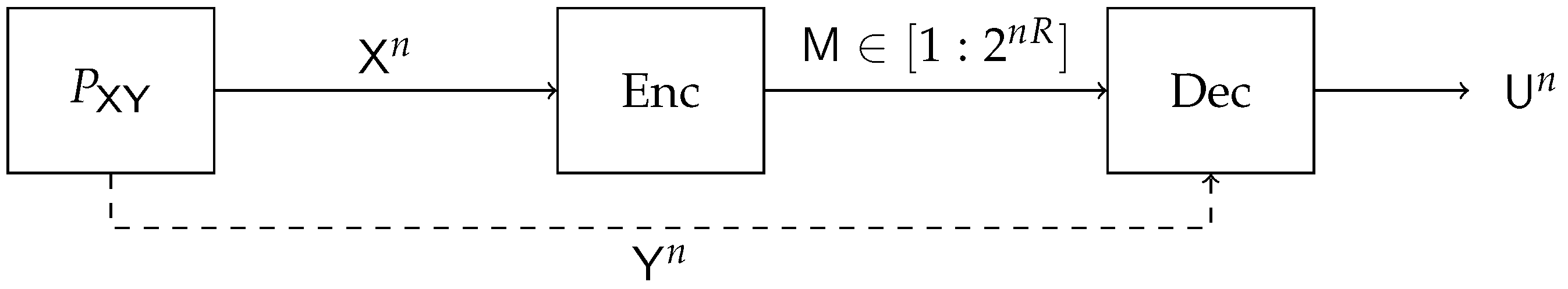
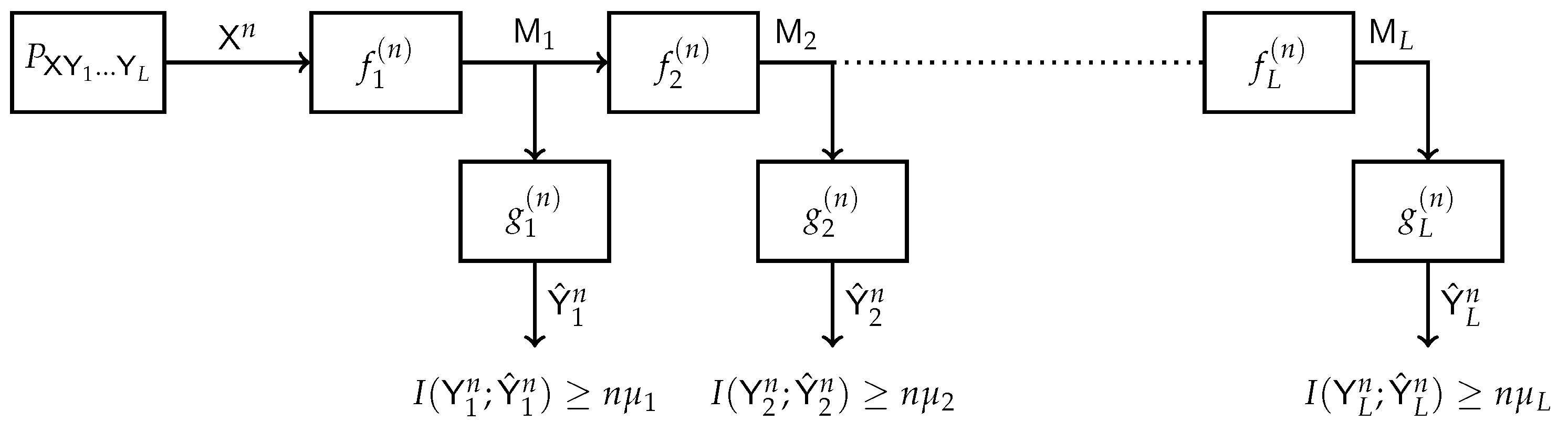
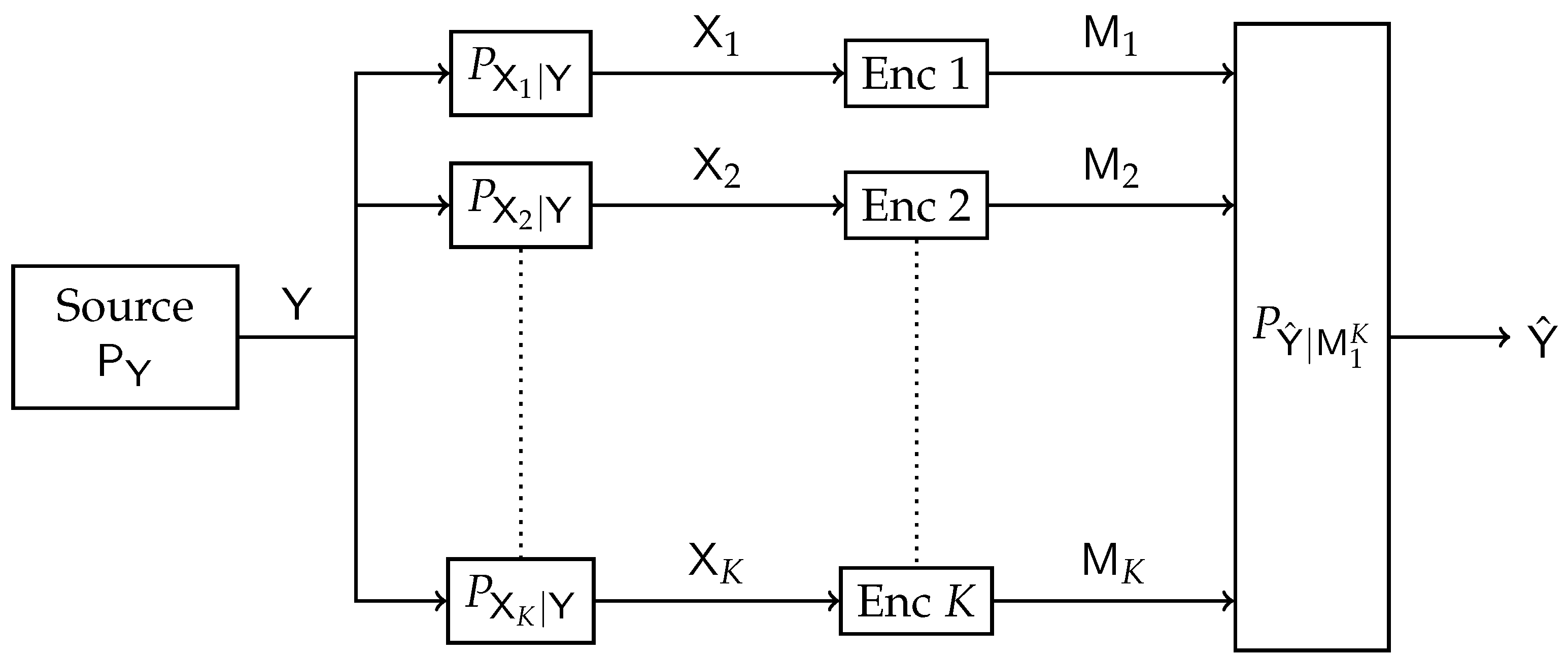
1.1. Related Work
1.2. Notations
1.3. Paper Outline
2. Problem Formulation and Basic Properties
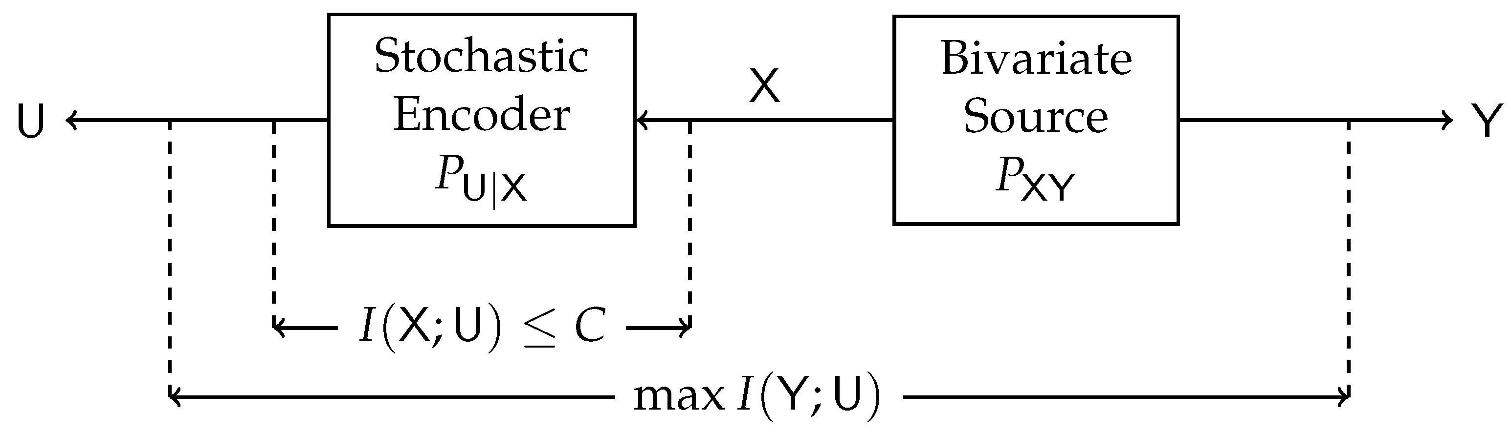
2.1. The Single-Sided Information Bottleneck (SSIB) Function
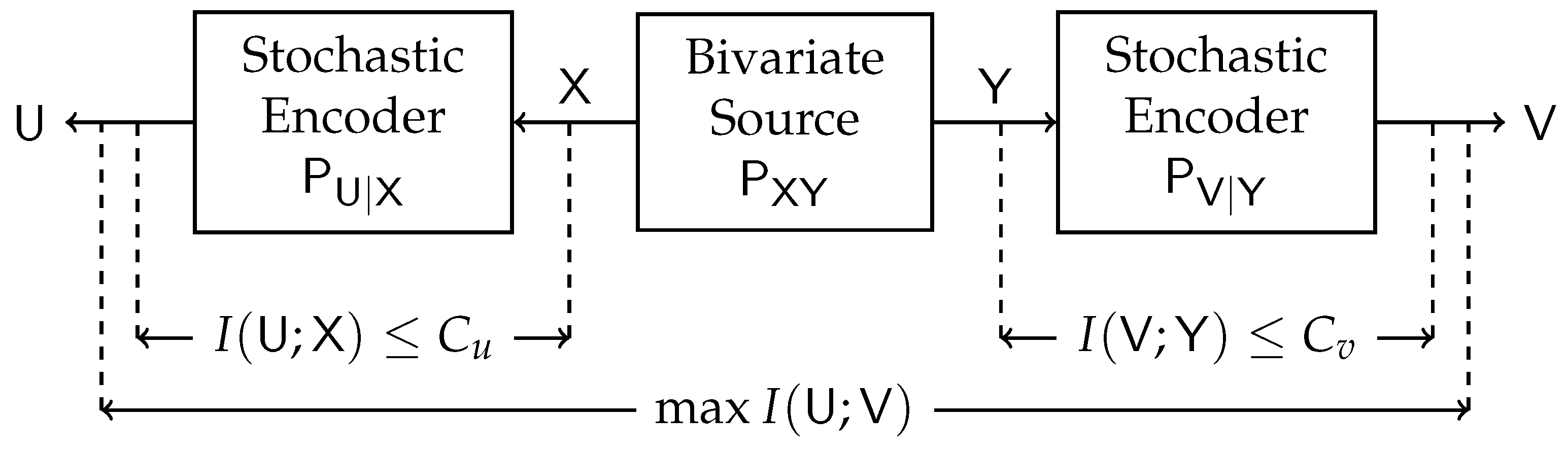
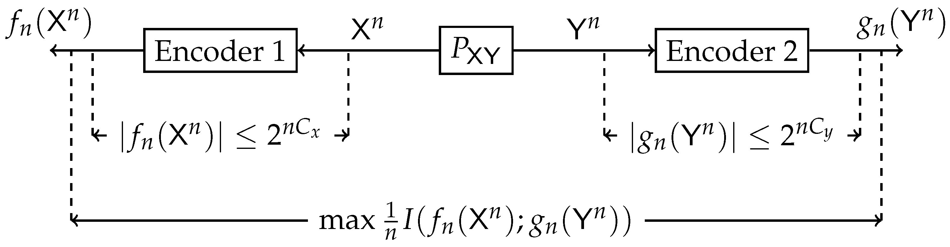
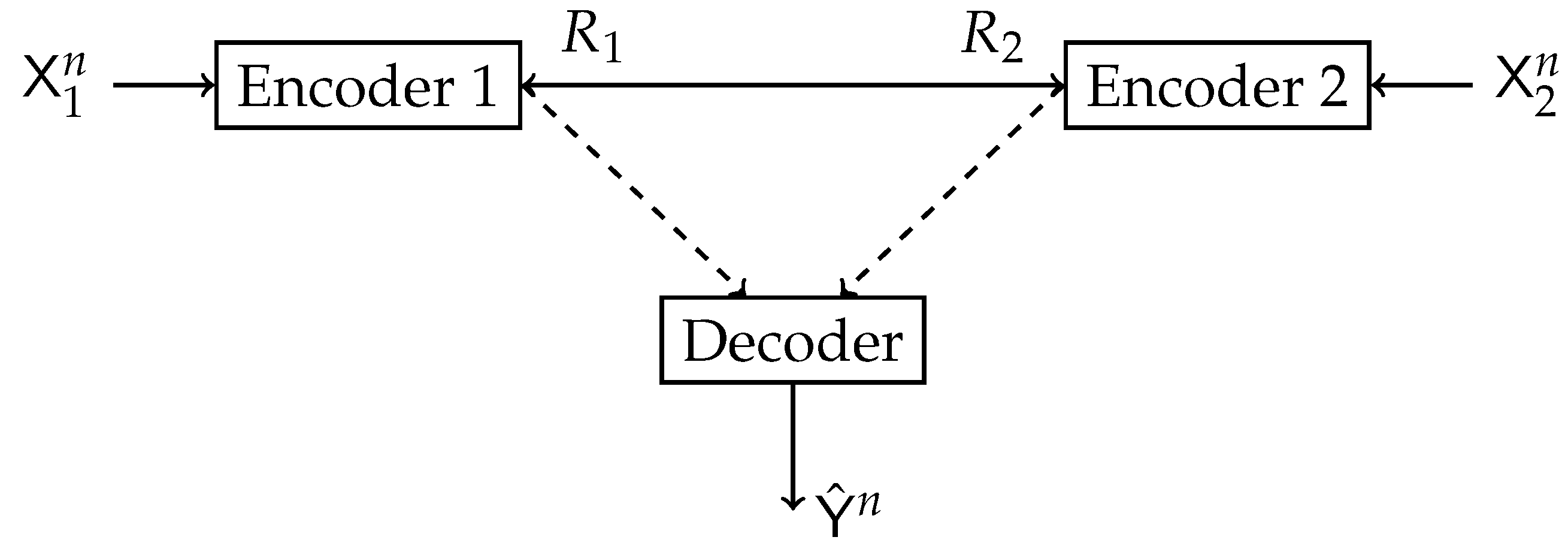
2.2. The Double-Sided Information Bottleneck (DSIB) Function
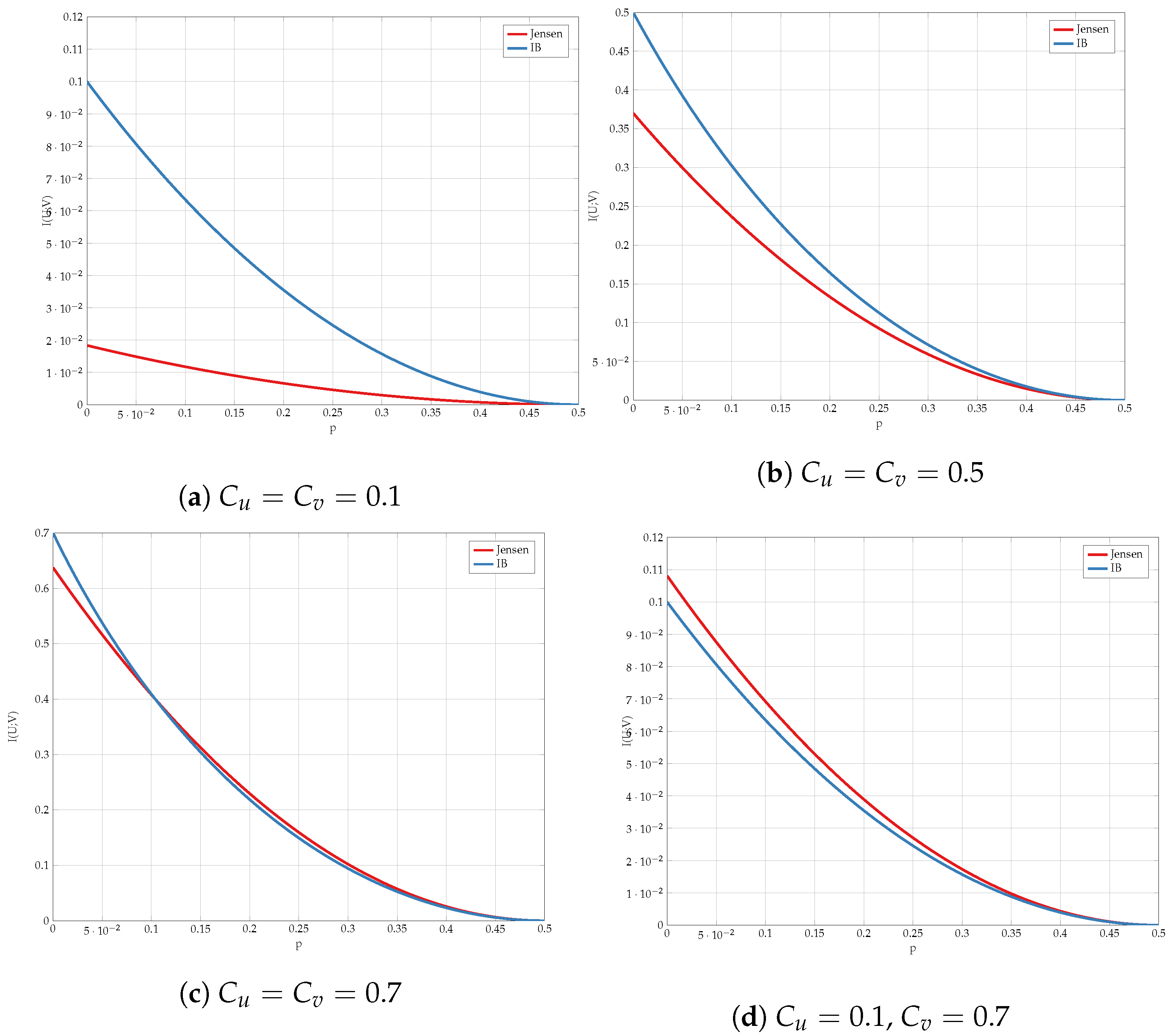
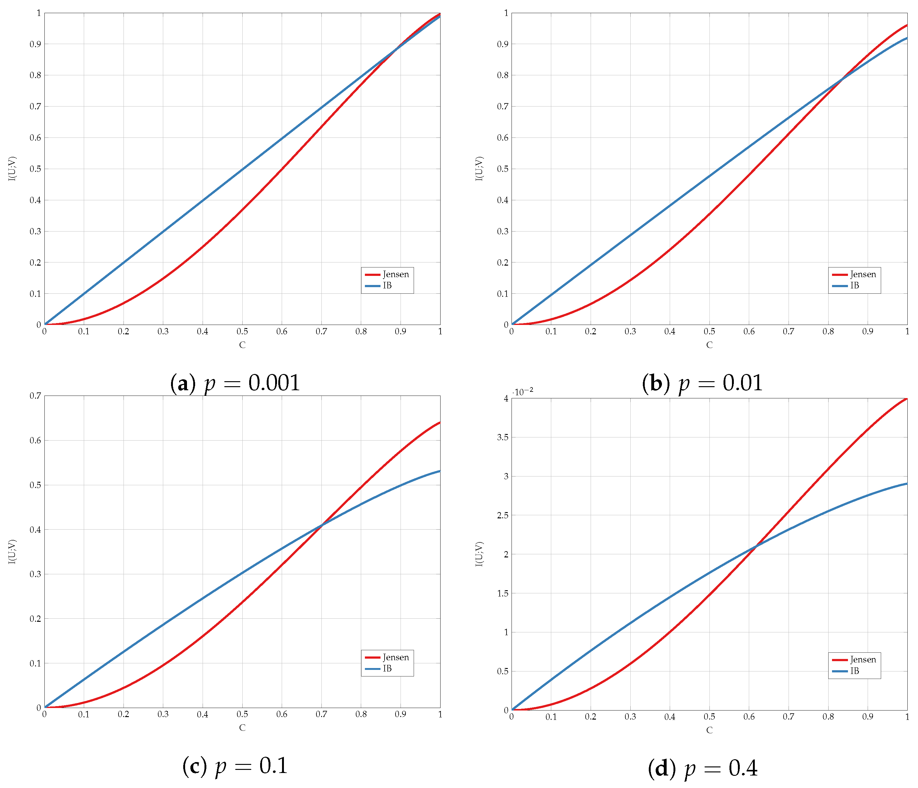
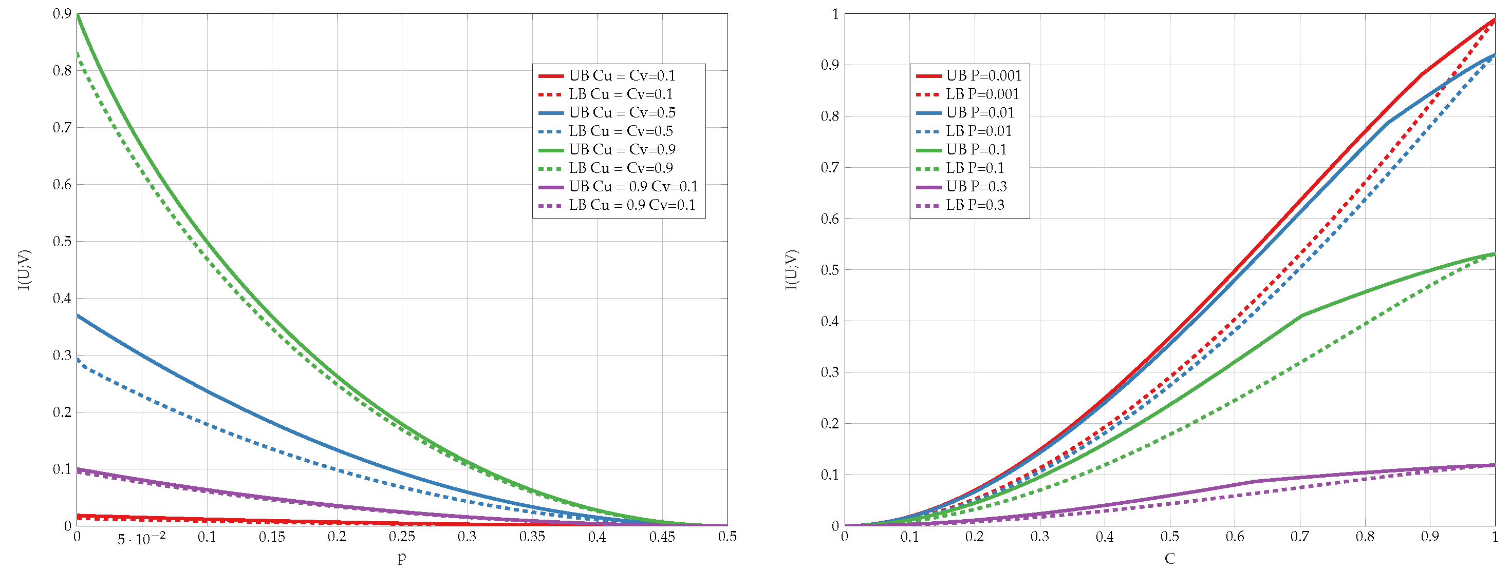
3. Binary
3.1. Special Cases
3.2. Bounds
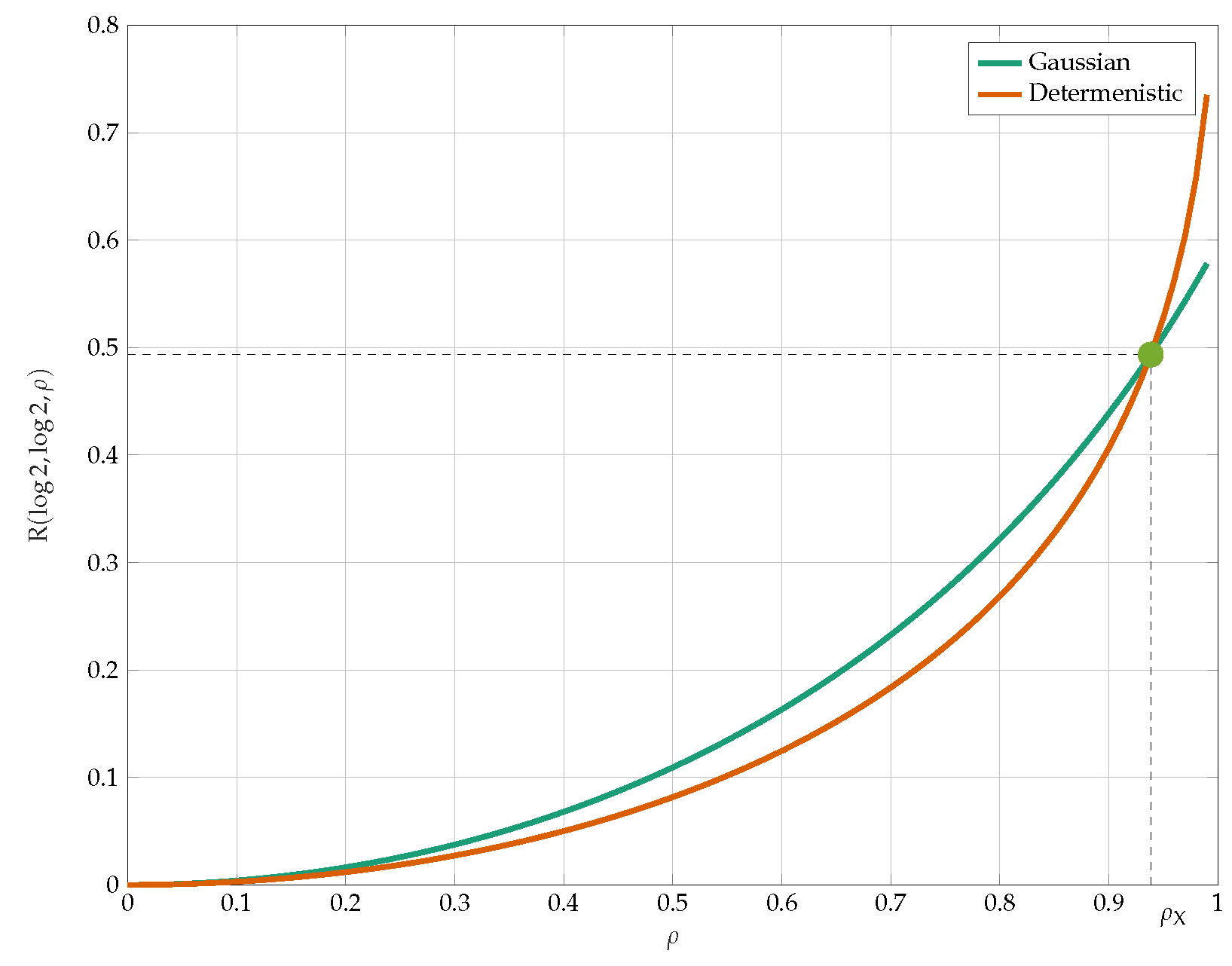
4. Gaussian
4.1. Low-SNR Regime
4.2. Optimality of Symbol-by-Symbol Quantization When
5. Alternating Maximization Algorithm
| Algorithm 1: IB iterative algorithm IBAM(args) |
 |
| Algorithm 2: DSIB iterative algorithm DSIBAM(args) |
 |
6. Numerical Results
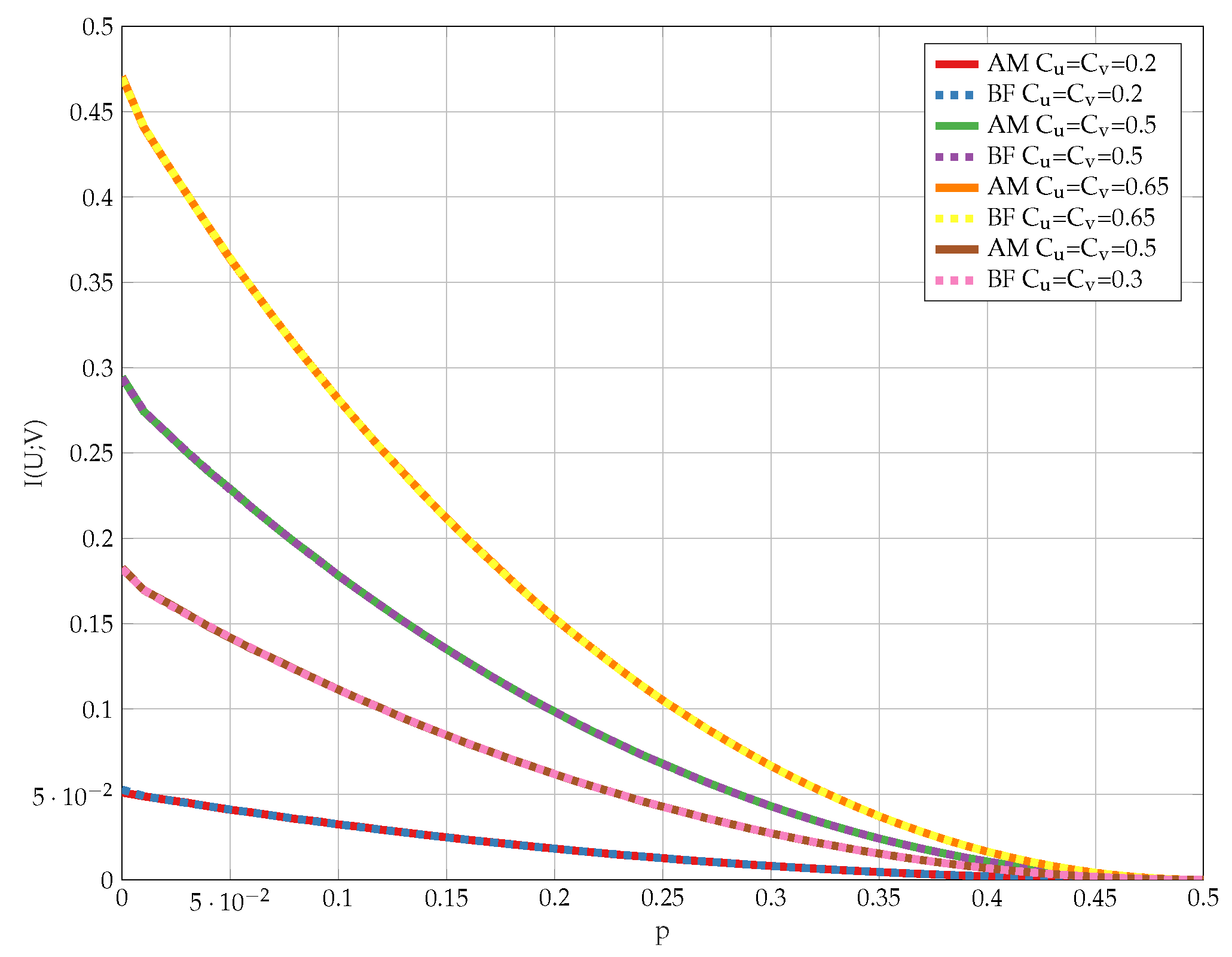
6.1. Exhaustive Search
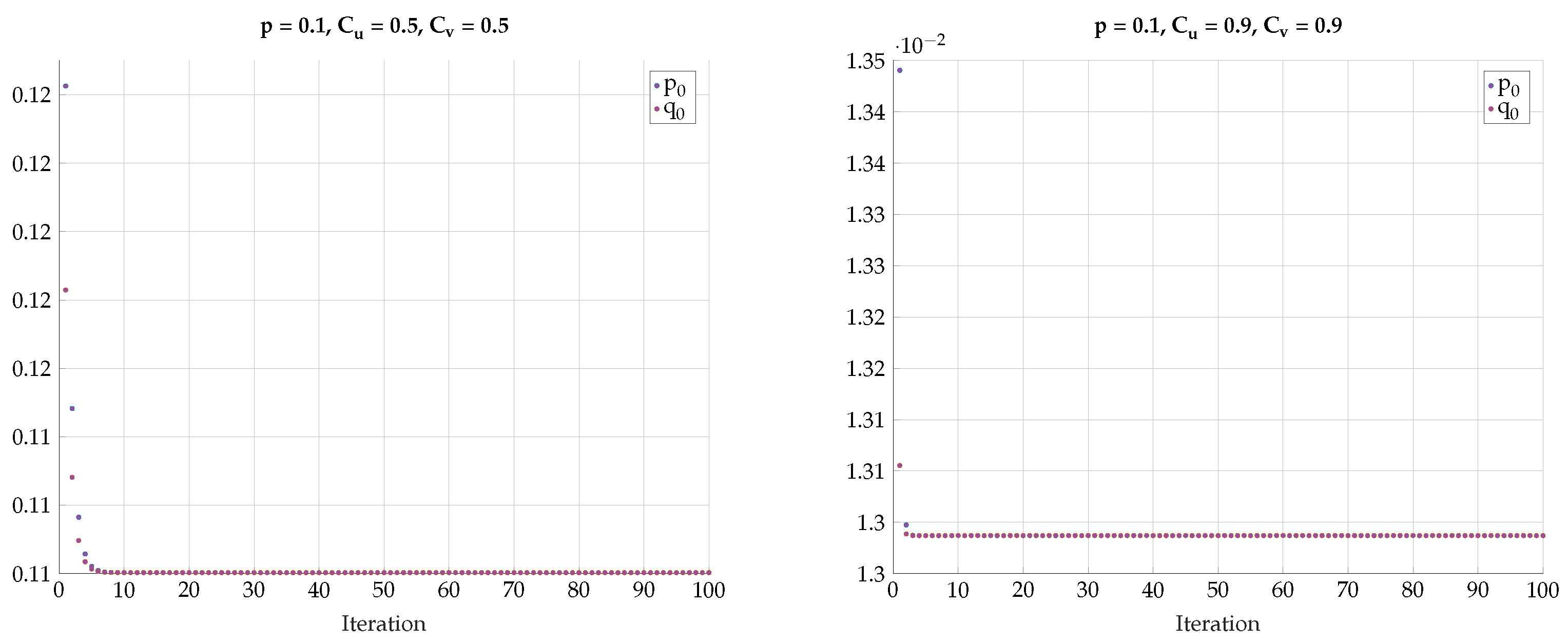
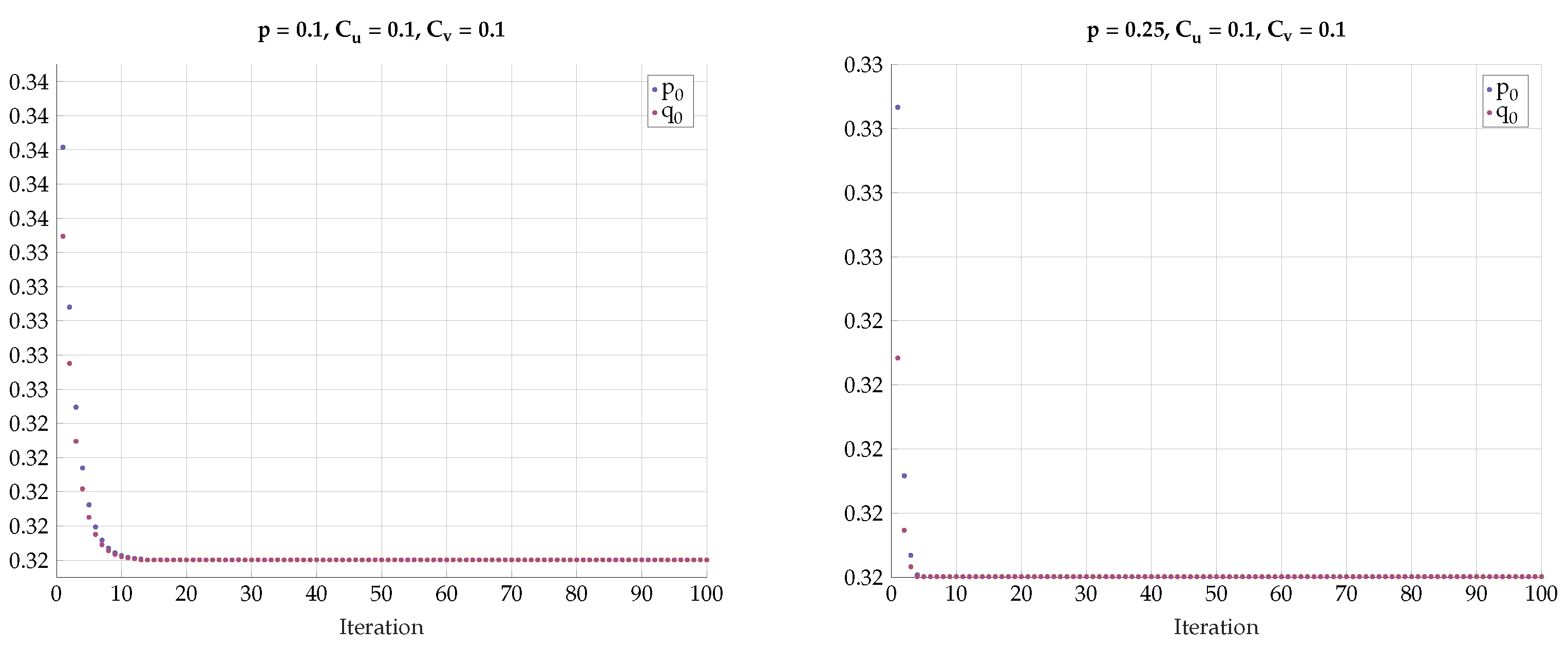
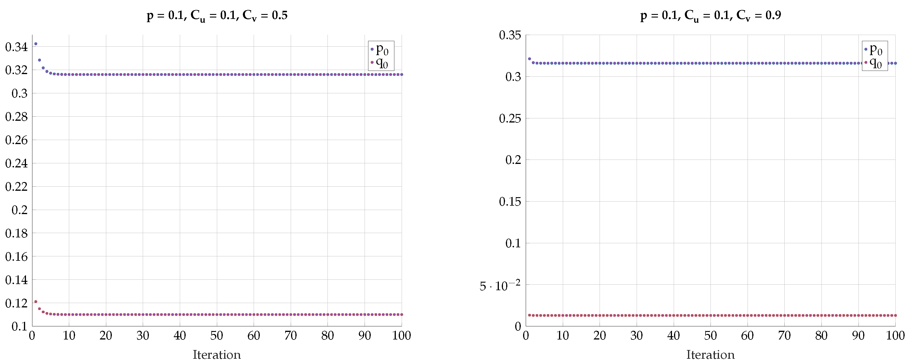
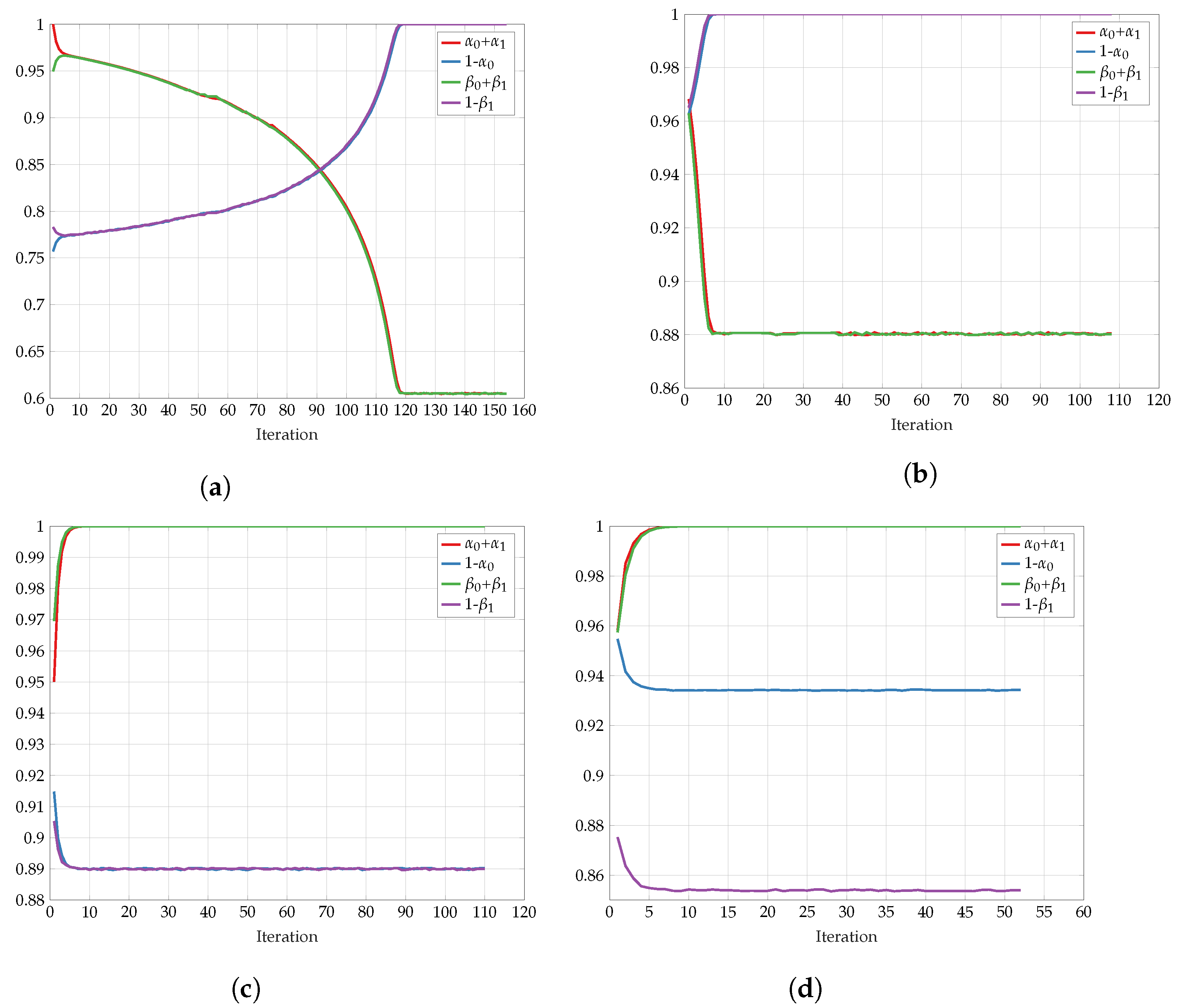
6.2. Alternating Maximization
7. Concluding Remarks
Author Contributions
Funding
Conflicts of Interest
Appendix A. Proof of Proposition 2
- 1.
- If is linear on a sub-interval of , then it is linear for every .
- 2.
- Otherwise, it is strictly convex over or there are points and such that where
Appendix B. Proof of Lemma 3
Appendix C. Auxiliary Concavity Lemma
Appendix D. Proof of Theorem 1
Appendix E. Proof of Proposition 4
Appendix F. Proof of Proposition 6
Appendix G. Proof of Proposition 7
Appendix H. Proof of Proposition 8
Appendix I. Proof of Proposition 9
Appendix J. Proof of Theorem 2
Appendix K. Proof of Lemma A1
- Suppose is linear over some interval . In such case, its second derivative must be zero over this interval, which implies that is zero over this interval. Since is a degree 3 polynomial, it can be zero over some interval if and only if it is zero everywhere. Thus, if is linear over some interval , then it is non-linear for every .
- For , and is a degree 3 polynomial in p. Since and , this polynomial has no sign changes or has exactly two sign changes in . Therefore, either is convex or there are two points and , , such that is convex in and concave in .
Appendix L. Proof of Lemma A2
Appendix M. Proof of Lemma A3
- , : This implies . Furthermore,which holds only if in contradiction to our initial assumption.
- , : This implieswhich holds only if . In such casein contradiction to the assumption .
References
- Tishby, N.; Pereira, F.C.N.; Bialek, W. The information bottleneck method. In Proceedings of the 37th Annual Allerton Conference on Communication, Control and Computing, Monticello, IL, USA, 22–24 September 1999; pp. 368–377. [Google Scholar]
- Pichler, G.; Piantanida, P.; Matz, G. Distributed information-theoretic clustering. Inf. Inference J. Ima 2021, 11, 137–166. [Google Scholar] [CrossRef]
- Jain, A.K.; Dubes, R.C. Algorithms for Clustering Data; Prentice-Hall: Hoboken, NJ, USA, 1988. [Google Scholar]
- Gupta, N.; Aggarwal, S. Modeling Biclustering as an optimization problem using Mutual Information. In Proceedings of the International Conference on Methods and Models in Computer Science (ICM2CS), Delhi, India, 14–15 December 2009; pp. 1–5. [Google Scholar]
- Hartigan, J. Direct Clustering of a Data Matrix. J. Am. Stat. Assoc. 1972, 67, 123–129. [Google Scholar] [CrossRef]
- Madeira, S.; Oliveira, A. Biclustering algorithms for biological data analysis: A survey. IEEE/ACM Trans. Comput. Biol. Bioinform. 2004, 1, 24–45. [Google Scholar] [CrossRef] [PubMed]
- Dhillon, I.S.; Mallela, S.; Modha, D.S. Information-Theoretic Co-Clustering. In Proceedings of the Ninth ACM SIGKDD International Conference on Knowledge Discovery and Data Mining, 2003, (KDD ’03), Washington, DC, USA, 24–27 August 2003; pp. 89–98. [Google Scholar]
- Courtade, T.A.; Kumar, G.R. Which Boolean Functions Maximize Mutual Information on Noisy Inputs? IEEE Trans. Inf. Theory 2014, 60, 4515–4525. [Google Scholar] [CrossRef]
- Han, T.S. Hypothesis Testing with Multiterminal Data Compression. IEEE Trans. Inf. Theory 1987, 33, 759–772. [Google Scholar] [CrossRef]
- Westover, M.B.; O’Sullivan, J.A. Achievable Rates for Pattern Recognition. IEEE Trans. Inf. Theory 2008, 54, 299–320. [Google Scholar] [CrossRef]
- Painsky, A.; Feder, M.; Tishby, N. An Information-Theoretic Framework for Non-linear Canonical Correlation Analysis. arXiv 2018, arXiv:1810.13259. [Google Scholar]
- Williamson, A.R. The Impacts of Additive Noise and 1-bit Quantization on the Correlation Coefficient in the Low-SNR Regime. In Proceedings of the 57th Annual Allerton Conference on Communication, Control, and Computing, Monticello, IL, USA, 24–27 September 2019; pp. 631–638. [Google Scholar]
- Courtade, T.A.; Weissman, T. Multiterminal Source Coding Under Logarithmic Loss. IEEE Trans. Inf. Theory 2014, 60, 740–761. [Google Scholar] [CrossRef]
- Pichler, G.; Piantanida, P.; Matz, G. Dictator Functions Maximize Mutual Information. Ann. Appl. Prob. 2018, 28, 3094–3101. [Google Scholar] [CrossRef]
- Dobrushin, R.; Tsybakov, B. Information transmission with additional noise. IRE Trans. Inf. Theory 1962, 8, 293–304. [Google Scholar] [CrossRef]
- Wolf, J.; Ziv, J. Transmission of noisy information to a noisy receiver with minimum distortion. IEEE Trans. Inf. Theory 1970, 16, 406–411. [Google Scholar] [CrossRef]
- Witsenhausen, H.S.; Wyner, A.D. A Conditional Entropy Bound for a Pair of Discrete Random Variables. IEEE Trans. Inf. Theory 1975, 21, 493–501. [Google Scholar] [CrossRef]
- Arimoto, S. An algorithm for computing the capacity of arbitrary discrete memoryless channels. IEEE Trans. Inf. Theory 1972, 18, 14–20. [Google Scholar] [CrossRef]
- Blahut, R. Computation of channel capacity and rate-distortion functions. IEEE Trans. Inf. Theory 1972, 18, 460–473. [Google Scholar] [CrossRef]
- Aguerri, I.E.; Zaidi, A. Distributed Variational Representation Learning. IEEE Trans. Pattern Anal. 2021, 43, 120–138. [Google Scholar] [CrossRef]
- Hassanpour, S.; Wuebben, D.; Dekorsy, A. Overview and Investigation of Algorithms for the Information Bottleneck Method. In Proceedings of the SCC 2017: 11th International ITG Conference on Systems, Communications and Coding, Hamburg, Germany, 6–9 February 2017; pp. 1–6. [Google Scholar]
- Slonim, N. The Information Bottleneck: Theory and Applications. Ph.D. Thesis, Hebrew University of Jerusalem, Jerusalem, Israel, 2002. [Google Scholar]
- Sutskover, I.; Shamai, S.; Ziv, J. Extremes of information combining. IEEE Trans. Inf. Theory 2005, 51, 1313–1325. [Google Scholar] [CrossRef]
- Zaidi, A.; Aguerri, I.E.; Shamai, S. On the Information Bottleneck Problems: Models, Connections, Applications and Information Theoretic Views. Entropy 2020, 22, 151. [Google Scholar] [CrossRef]
- Wyner, A.; Ziv, J. A theorem on the entropy of certain binary sequences and applications–I. IEEE Trans. Inf. Theory 1973, 19, 769–772. [Google Scholar] [CrossRef]
- Chechik, G.; Globerson, A.; Tishby, N.; Weiss, Y. Information Bottleneck for Gaussian Variables. J. Mach. Learn. Res. 2005, 6, 165–188. [Google Scholar]
- Blachman, N. The convolution inequality for entropy powers. IEEE Trans. Inf. Theory 1965, 11, 267–271. [Google Scholar] [CrossRef]
- Guo, D.; Shamai, S.; Verdú, S. The interplay between information and estimation measures. Found. Trends Signal Process. 2013, 6, 243–429. [Google Scholar] [CrossRef]
- Bustin, R.; Payaro, M.; Palomar, D.P.; Shamai, S. On MMSE Crossing Properties and Implications in Parallel Vector Gaussian Channels. IEEE Trans. Inf. Theory 2013, 59, 818–844. [Google Scholar] [CrossRef]
- Sanderovich, A.; Shamai, S.; Steinberg, Y.; Kramer, G. Communication Via Decentralized Processing. IEEE Trans. Inf. Theory 2008, 54, 3008–3023. [Google Scholar] [CrossRef]
- Smith, J.G. The information capacity of amplitude-and variance-constrained scalar Gaussian channels. Inf. Control. 1971, 18, 203–219. [Google Scholar] [CrossRef]
- Sharma, N.; Shamai, S. Transition points in the capacity-achieving distribution for the peak-power limited AWGN and free-space optical intensity channels. Probl. Inf. Transm. 2010, 46, 283–299. [Google Scholar] [CrossRef]
- Dytso, A.; Yagli, S.; Poor, H.V.; Shamai, S. The Capacity Achieving Distribution for the Amplitude Constrained Additive Gaussian Channel: An Upper Bound on the Number of Mass Points. IEEE Trans. Inf. Theory 2019, 66, 2006–2022. [Google Scholar] [CrossRef]
- Steinberg, Y. Coding and Common Reconstruction. IEEE Trans. Inf. Theory 2009, 55, 4995–5010. [Google Scholar] [CrossRef]
- Land, I.; Huber, J. Information Combining. Found. Trends Commun. Inf. Theory 2006, 3, 227–330. [Google Scholar] [CrossRef]
- Yang, Q.; Piantanida, P.; Gündüz, D. The Multi-layer Information Bottleneck Problem. In Proceedings of the IEEE Information Theory Workshop (ITW), Kaohsiung, Taiwan, 6–10 November 2017; pp. 404–408. [Google Scholar]
- Berger, T.; Zhang, Z.; Viswanathan, H. The CEO Problem. IEEE Trans. Inf. Theory 1996, 42, 887–902. [Google Scholar] [CrossRef]
- Steiner, S.; Kuehn, V. Optimization Of Distributed Quantizers Using An Alternating Information Bottleneck Approach. In Proceedings of the WSA 2019: 23rd International ITG Workshop on Smart Antennas, Vienna, Austria, 24–26 April 2019; pp. 1–6. [Google Scholar]
- Vera, M.; Rey Vega, L.; Piantanida, P. Collaborative Information Bottleneck. IEEE Trans. Inf. Theory 2019, 65, 787–815. [Google Scholar] [CrossRef]
- Ugur, Y.; Aguerri, I.E.; Zaidi, A. Vector Gaussian CEO Problem Under Logarithmic Loss and Applications. IEEE Trans. Inf. Theory 2020, 66, 4183–4202. [Google Scholar] [CrossRef]
- Estella, I.; Zaidi, A. Distributed Information Bottleneck Method for Discrete and Gaussian Sources. In Proceedings of the International Zurich Seminar on Information and Communication (IZS), Zurich, Switzerland, 21–23 February 2018; pp. 35–39. [Google Scholar]
- Courtade, T.A.; Jiao, J. An Extremal Inequality for Long Markov Chains. In Proceedings of the 52nd Annual Allerton Conference on Communication, Control, and Computing, Monticello, IL, USA, 1–3 October 2014; pp. 763–770. [Google Scholar]
- Erkip, E.; Cover, T.M. The Efficiency of Investment Information. IEEE Trans. Inf. Theory 1998, 44, 1026–1040. [Google Scholar] [CrossRef]
- Gács, P.; Körner, J. Common information is far less than mutual information. Probl. Contr. Inform. Theory 1973, 2, 149–162. [Google Scholar]
- Farajiparvar, P.; Beirami, A.; Nokleby, M. Information Bottleneck Methods for Distributed Learning. In Proceedings of the 56th Annual Allerton Conference on Communication, Control, and Computing, Monticello, IL, USA, 2–5 October 2018; pp. 24–31. [Google Scholar]
- Tishby, N.; Zaslavsky, N. Deep Learning and the Information Bottleneck Principle. In Proceedings of the Information Theory Workshop (ITW), Jeju Island, Korea, 11–15 October 2015; pp. 1–5. [Google Scholar]
- Alemi, A.; Fischer, I.; Dillon, J.; Murphy, K. Deep Variational Information Bottleneck. In Proceedings of the International Conference on Learning Representations (ICLR), Toulon, France, 24–26 April 2017. [Google Scholar]
- Shwartz-Ziv, R.; Tishby, N. Opening the black box of deep neural networks via information. arXiv 2017, arXiv:1703.00810. [Google Scholar]
- Gabrié, M.; Manoel, A.; Luneau, C.; Barbier, j.; Macris, N.; Krzakala, F.; Zdeborová, L. Entropy and mutual information in models of deep neural networks. In Advances in NIPS; Curran Associates, Inc.: Red Hook, NY, USA, 2018; Volume 31. [Google Scholar]
- Goldfeld, Z.; van den Berg, E.; Greenewald, K.H.; Melnyk, I.; Nguyen, N.; Kingsbury, B.; Polyanskiy, Y. Estimating Information Flow in Neural Networks. arXiv 2018, arXiv:1810.05728. [Google Scholar]
- Amjad, R.A.; Geiger, B.C. Learning Representations for Neural Network-Based Classification Using the Information Bottleneck Principle. IEEE Trans. Pattern Anal. 2020, 42, 2225–2239. [Google Scholar] [CrossRef]
- Saxe, A.M.; Bansal, Y.; Dapello, J.; Advani, M.; Kolchinsky, A.; Tracey, B.D.; Cox, D.D. On the information bottleneck theory of deep learning. J. Stat. Mech. Theory Exp. 2019, 2019, 1–34. [Google Scholar] [CrossRef]
- Cheng, H.; Lian, D.; Gao, S.; Geng, Y. Evaluating Capability of Deep Neural Networks for Image Classification via Information Plane. In Lecture Notes in Computer Science, Proceedings of the Computer Vision-ECCV 2018-15th European Conference, Munich, Germany, 8–14 September 2018, Proceedings, Part XI; Ferrari, V., Hebert, M., Sminchisescu, C., Weiss, Y., Eds.; Springer: Berlin/Heidelberg, Germany, 2018; Volume 11215, pp. 181–195. [Google Scholar]
- Yu, S.; Wickstrøm, K.; Jenssen, R.; Príncipe, J.C. Understanding Convolutional Neural Networks with Information Theory: An Initial Exploration. IEEE Trans. Neural Netw. Learn. Syst. 2021, 32, 435–442. [Google Scholar] [CrossRef]
- Lewandowsky, J.; Stark, M.; Bauch, G. Information bottleneck graphs for receiver design. In Proceedings of the IEEE International Symposium on Information Theory, Barcelona, Spain, 10–15 July 2016; pp. 2888–2892. [Google Scholar]
- Stark, M.; Wang, L.; Bauch, G.; Wesel, R.D. Decoding rate-compatible 5G-LDPC codes with coarse quantization using the information bottleneck method. IEEE Open J. Commun. Soc. 2020, 1, 646–660. [Google Scholar] [CrossRef]
- Bhatt, A.; Nazer, B.; Ordentlich, O.; Polyanskiy, Y. Information-distilling quantizers. IEEE Trans. Inf. Theory 2021, 67, 2472–2487. [Google Scholar] [CrossRef]
- Stark, M.; Shah, A.; Bauch, G. Polar code construction using the information bottleneck method. In Proceedings of the 2018 IEEE Wireless Communications and Networking Conference Workshops (WCNCW), Barcelona, Spain, 15–18 April 2018; pp. 7–12. [Google Scholar]
- Shah, S.A.A.; Stark, M.; Bauch, G. Design of Quantized Decoders for Polar Codes using the Information Bottleneck Method. In Proceedings of the SCC 2019: 12th International ITG Conference on Systems, Communications and Coding, Rostock, Germany, 11–14 February 2019; pp. 1–6. [Google Scholar]
- Shah, S.A.A.; Stark, M.; Bauch, G. Coarsely Quantized Decoding and Construction of Polar Codes Using the Information Bottleneck Method. Algorithms 2019, 12, 192. [Google Scholar] [CrossRef]
- Kurkoski, B.M. On the Relationship Between the KL Means Algorithm and the Information Bottleneck Method. In Proceedings of the 11th International ITG Conference on Systems, Communications and Coding (SCC), Hamburg, Germany, 6–9 February 2017; pp. 1–6. [Google Scholar]
- Goldfeld, Z.; Polyanskiy, Y. The Information Bottleneck Problem and its Applications in Machine Learning. IEEE J. Sel. Areas Inf. Theory 2020, 1, 19–38. [Google Scholar] [CrossRef]
- Harremoes, P.; Tishby, N. The Information Bottleneck Revisited or How to Choose a Good Distortion Measure. In Proceedings of the 2007 IEEE International Symposium on Information Theory, Nice, France, 24–29 June 2007; pp. 566–570. [Google Scholar]
- Richardson, T.; Urbanke, R. Modern Coding Theory; Cambridge University Press: Cambridge, UK, 2008. [Google Scholar]
- Sason, I. On f-divergences: Integral representations, local behavior, and inequalities. Entropy 2018, 20, 383. [Google Scholar] [CrossRef] [PubMed]
- Mehler, F.G. Ueber die Entwicklung einer Function von beliebig vielen Variablen nach Laplaceschen Functionen höherer Ordnung. J. Reine Angew. Math. 1866, 66, 161–176. [Google Scholar]
- Lancaster, H.O. The Structure of Bivariate Distributions. Ann. Math. Statist. 1958, 29, 719–736. [Google Scholar] [CrossRef]
- O’Donnell, R. Analysis of Boolean Functions, 1st ed.; Cambridge University Press: New York, NY, USA, 2014. [Google Scholar]
- Cover, T.M.; Thomas, J.A. Elements of Information Theory; Wiley: Hoboken, NJ, USA, 2006. [Google Scholar]
- Corless, M.J. Linear Systems and Control : An Operator Perspective; Monographs and Textbooks in Pure and Applied Mathematics; Marcel Dekker: New York, NY, USA, 2003; Volume 254. [Google Scholar]


Publisher’s Note: MDPI stays neutral with regard to jurisdictional claims in published maps and institutional affiliations. |
© 2022 by the authors. Licensee MDPI, Basel, Switzerland. This article is an open access article distributed under the terms and conditions of the Creative Commons Attribution (CC BY) license (https://creativecommons.org/licenses/by/4.0/).
Share and Cite
Dikshtein, M.; Ordentlich, O.; Shamai, S. The Double-Sided Information Bottleneck Function. Entropy 2022, 24, 1321. https://doi.org/10.3390/e24091321
Dikshtein M, Ordentlich O, Shamai S. The Double-Sided Information Bottleneck Function. Entropy. 2022; 24(9):1321. https://doi.org/10.3390/e24091321
Chicago/Turabian StyleDikshtein, Michael, Or Ordentlich, and Shlomo Shamai (Shitz). 2022. "The Double-Sided Information Bottleneck Function" Entropy 24, no. 9: 1321. https://doi.org/10.3390/e24091321