
A Novel Bearing Fault Diagnosis Method Based on Few-Shot Transfer Learning across Different Datasets

Abstract
:1. Introduction
- (1)
- In view of the problems that most of the current intelligent fault diagnosis methods cannot be directly applied to industry, a few-shot transfer learning method across different datasets is proposed, which can use the diagnostic knowledge learned from ASF data to effectively identify the health state of the new machine bearings.
- (2)
- For the first time, a very small number of target domain samples are used to replace the original samples of the support set in fault diagnosis, which improves the generalization ability of the model, and has very high stability and accuracy even in different datasets (ASF-NF) with great differences in feature space distribution.
- (3)
- Several experiments are designed to compare and verify many aspects of the proposed method, which has achieved the expected results, and our method does not need secondary training, which will be more convenient.
2. Basic Theory
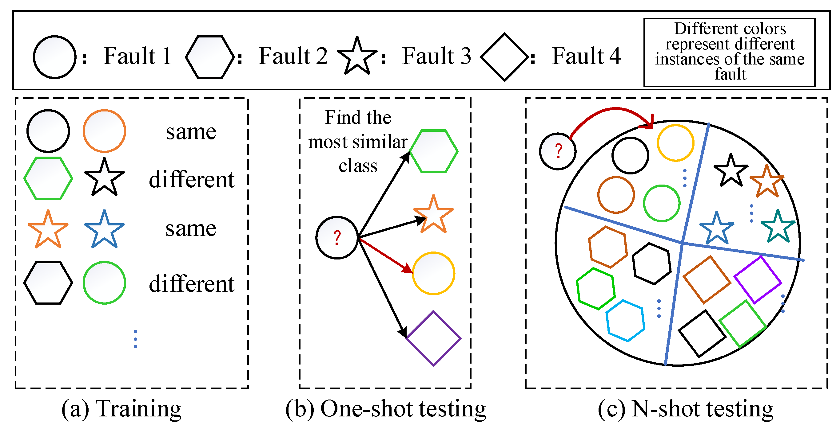
2.1. Few-Shot Learning Strategy
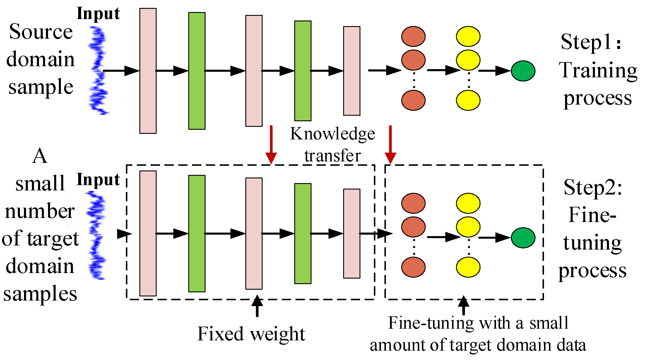
2.2. Fine-Tuning-Based Method
3. The Proposed Method
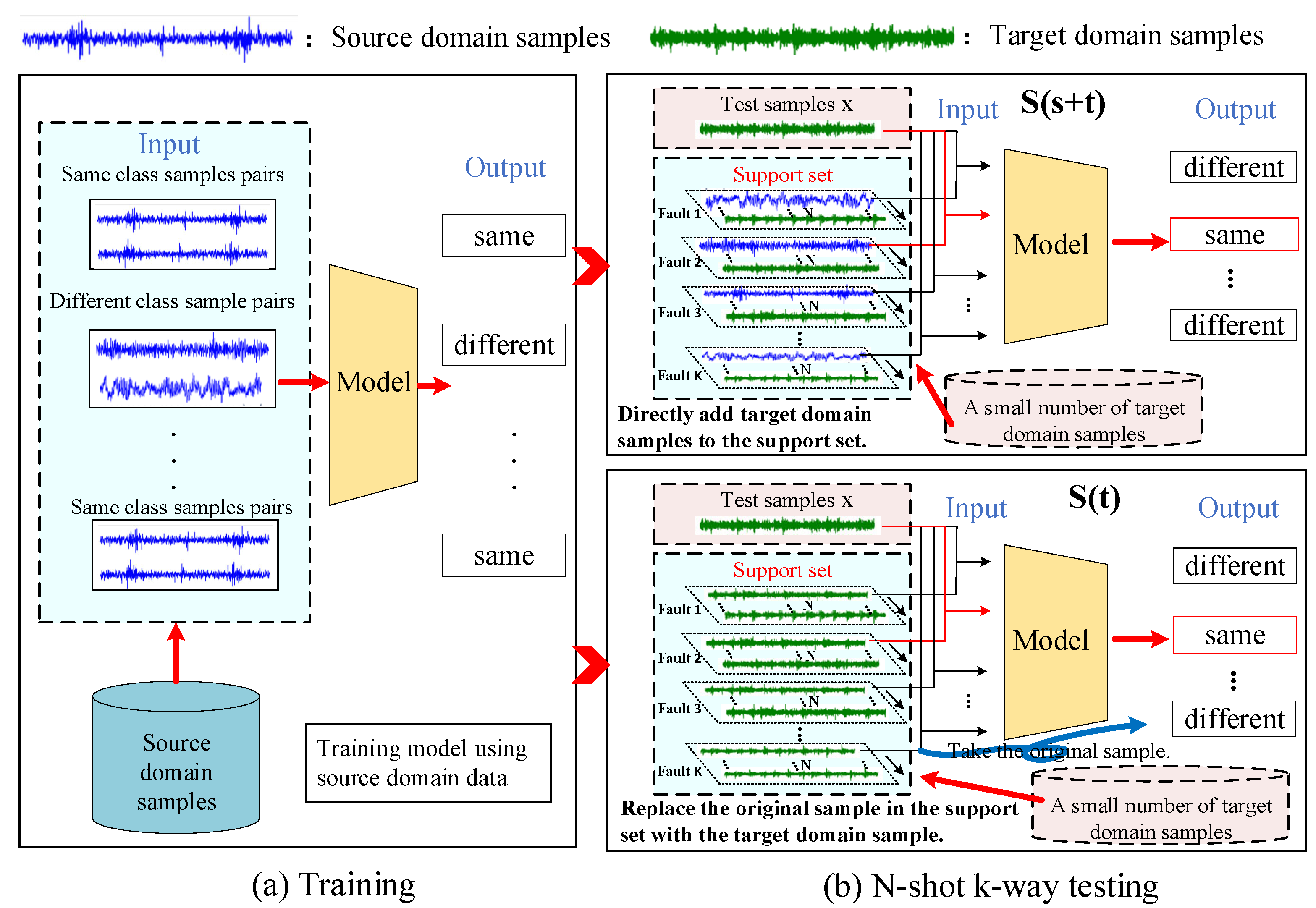
3.1. The Proposed Few-Shot Transfer Learning Methods
- (1)
- S(s+t): Directly add target domain samples to the support set.
- (2)
- S(t): Replace the original sample in the support set with the target domain sample.
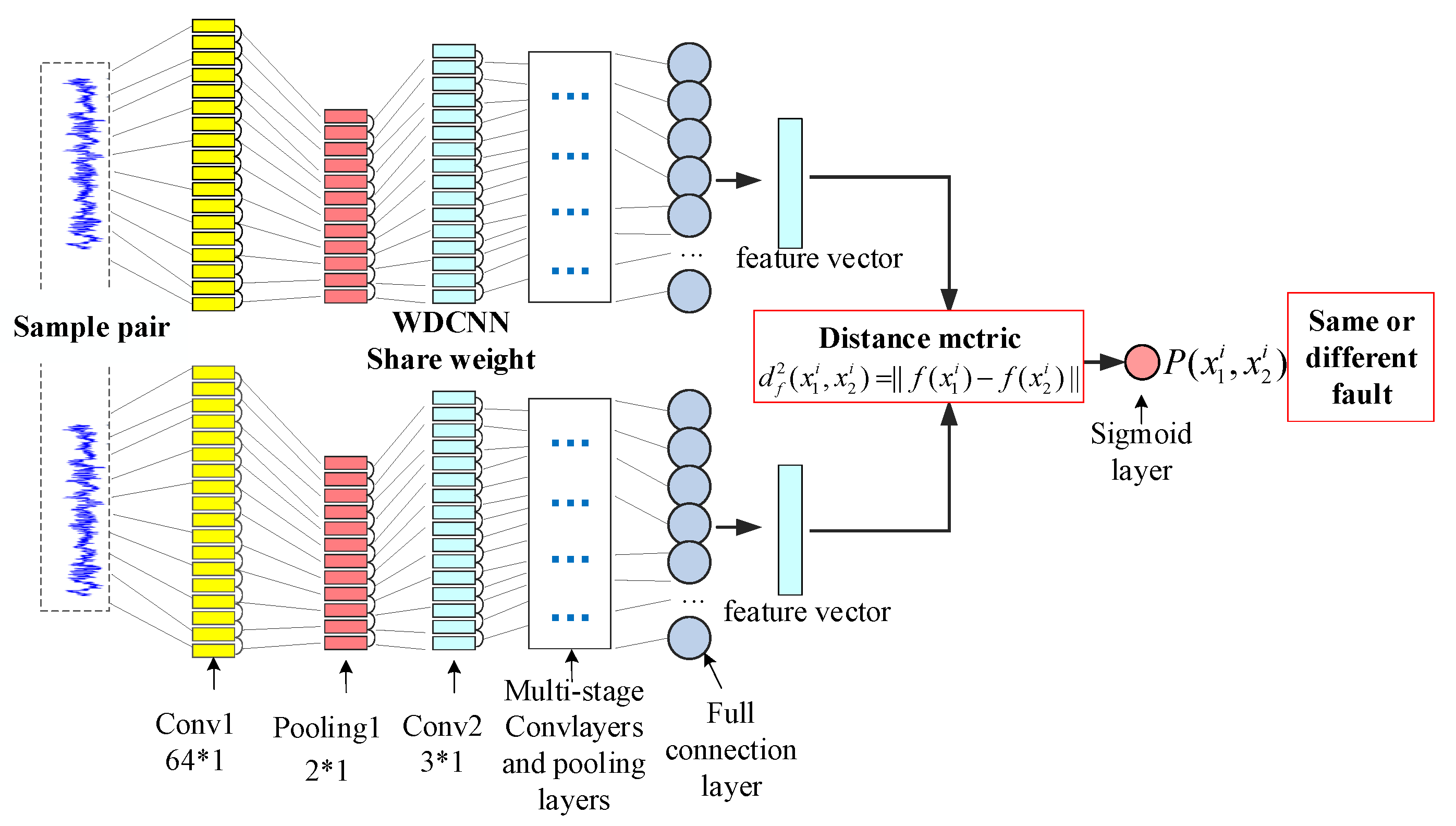
3.2. Model
4. Experiment and Results
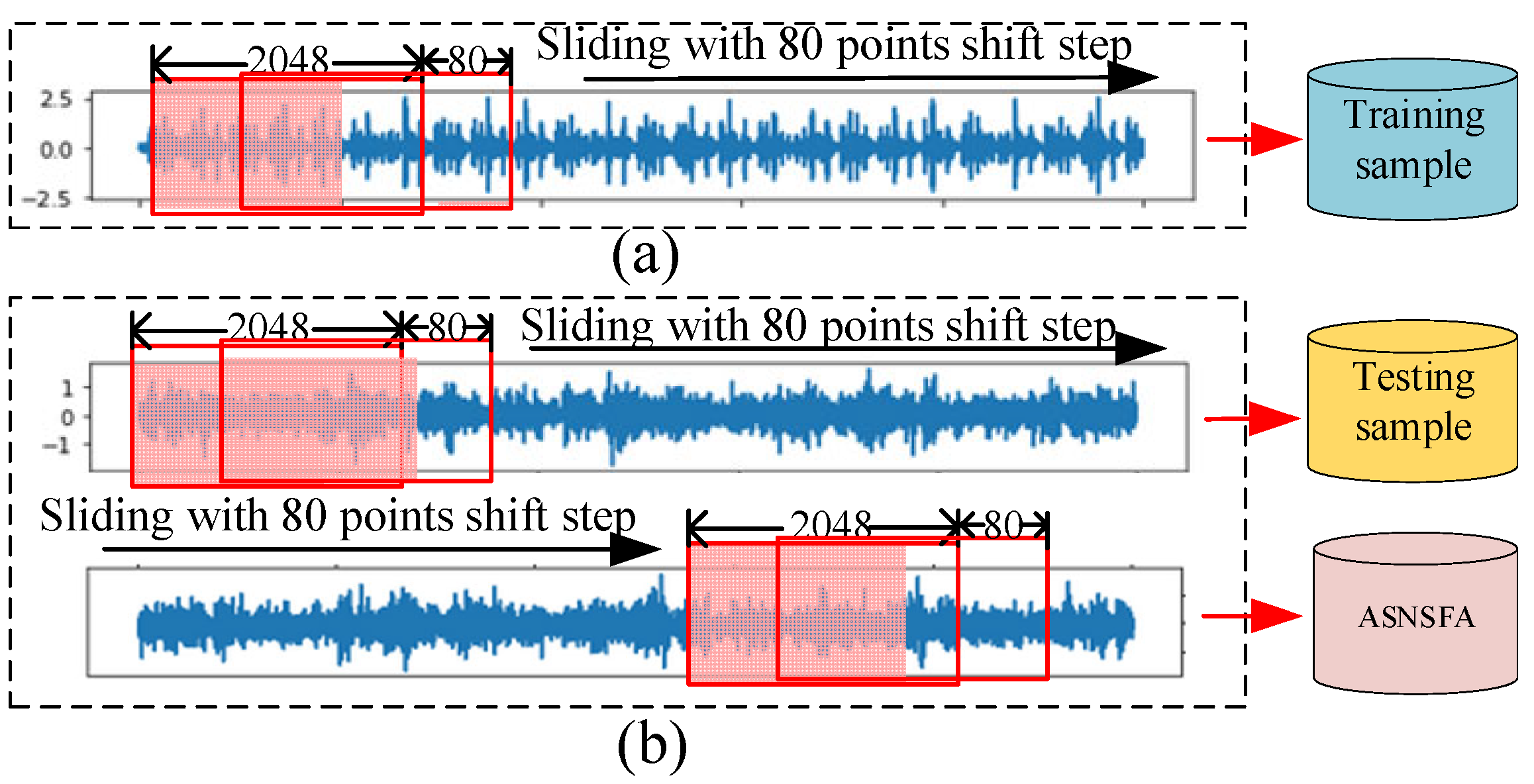
4.1. Data Introduction and Processing
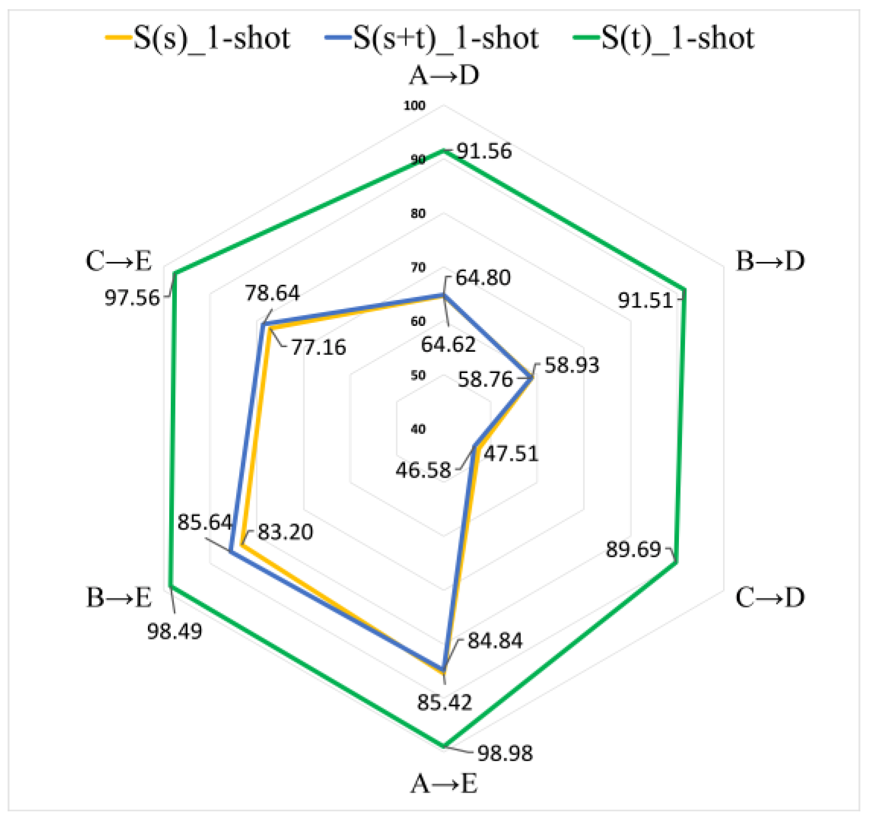
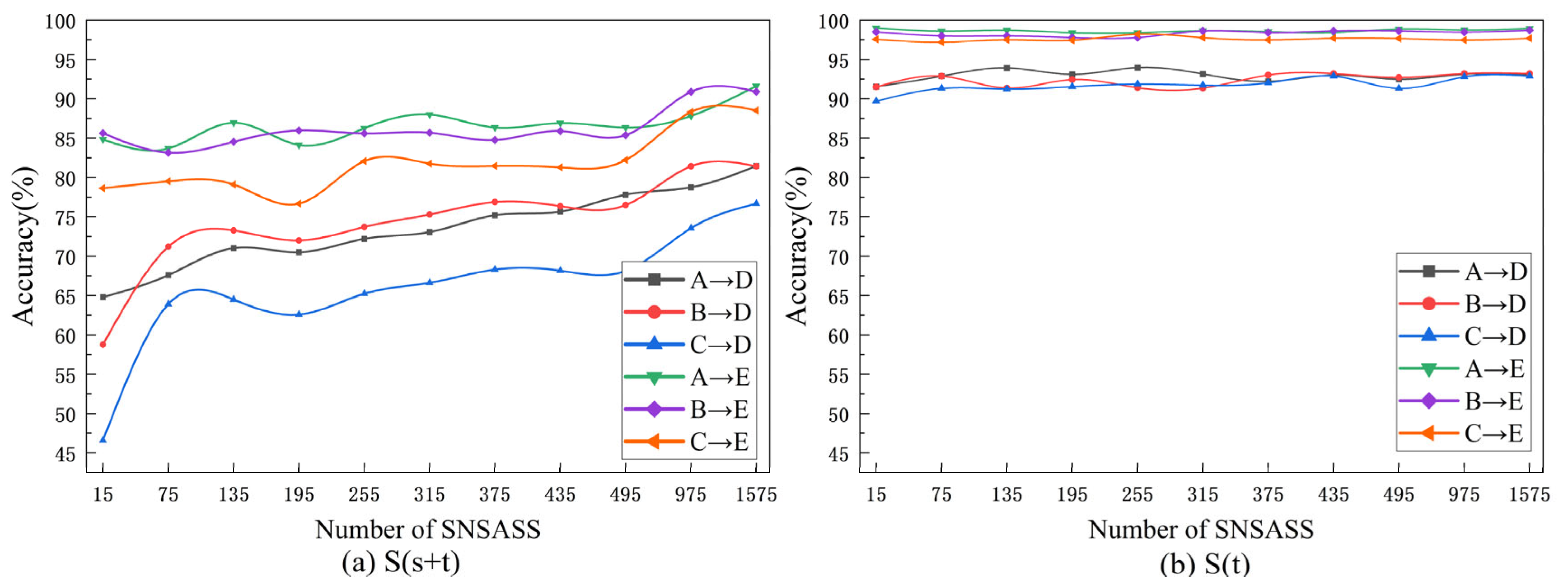
4.2. S(s), S(s+t) and S(t) Analysis
- (1)
- S(s): direct transfer method (baseline).
- (2)
- S(s+t): directly add target domain samples to the support set.
- (3)
- S(t): replace the original samples in the support set with the target domain samples.
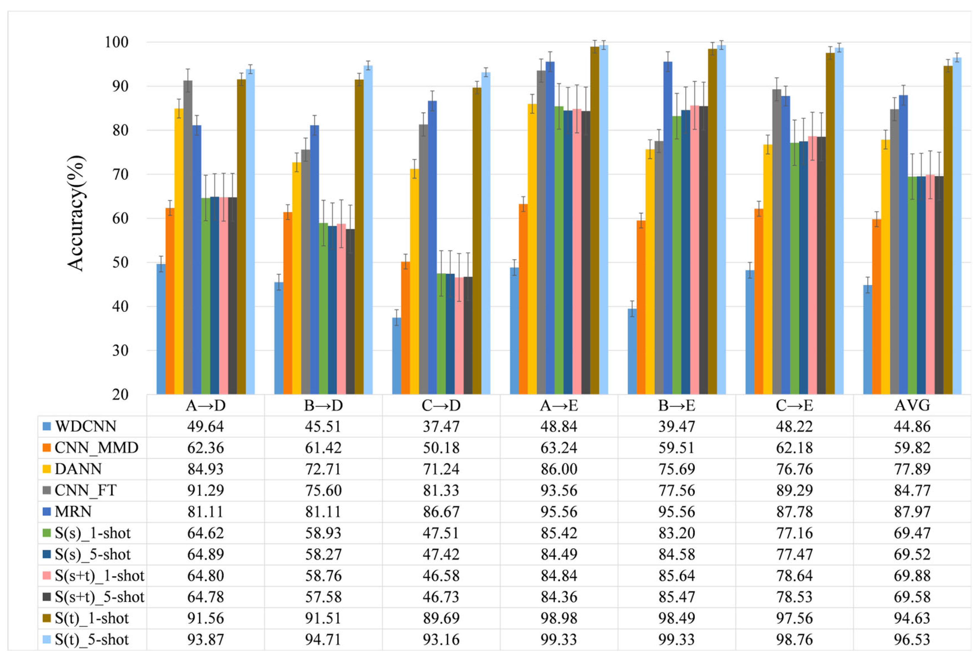
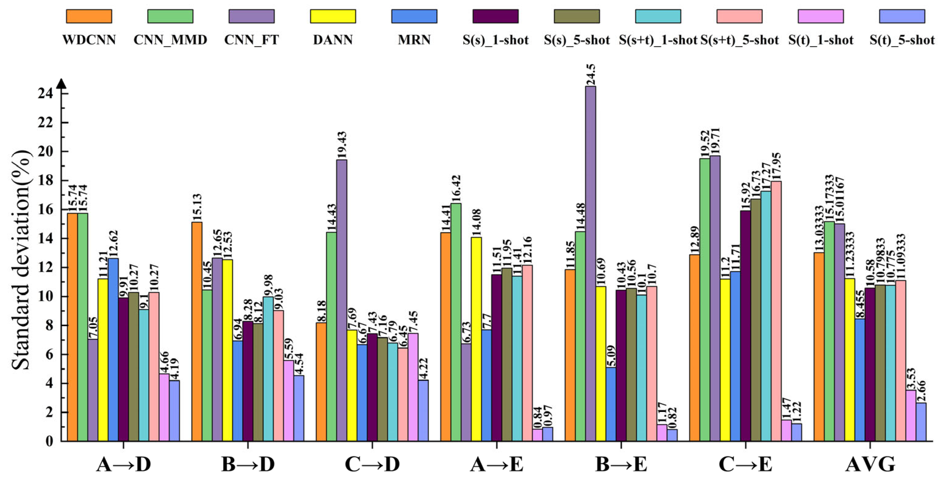
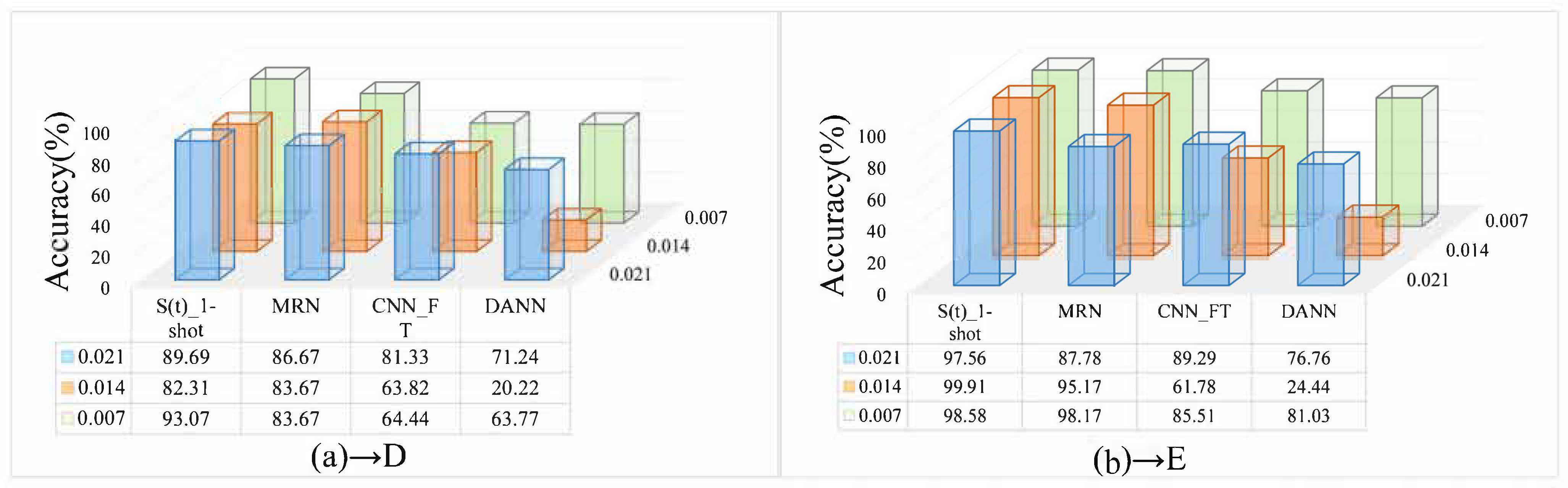
4.3. Comparisons with Other Methods
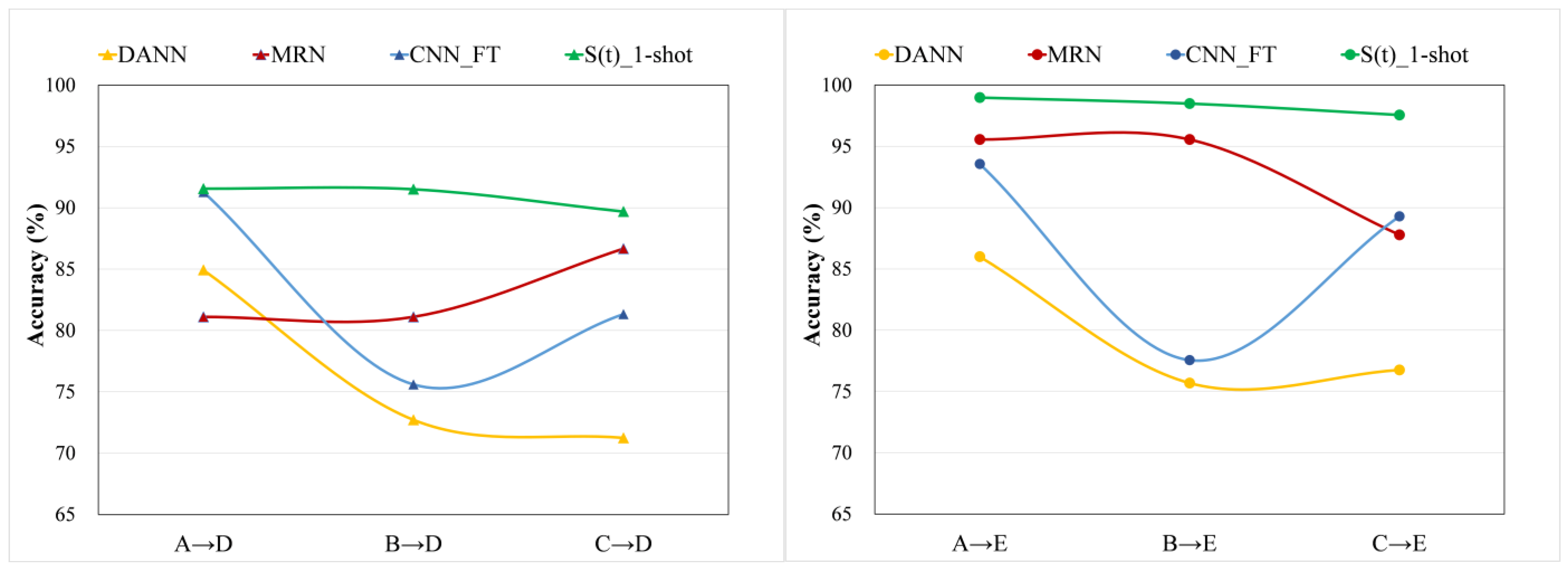
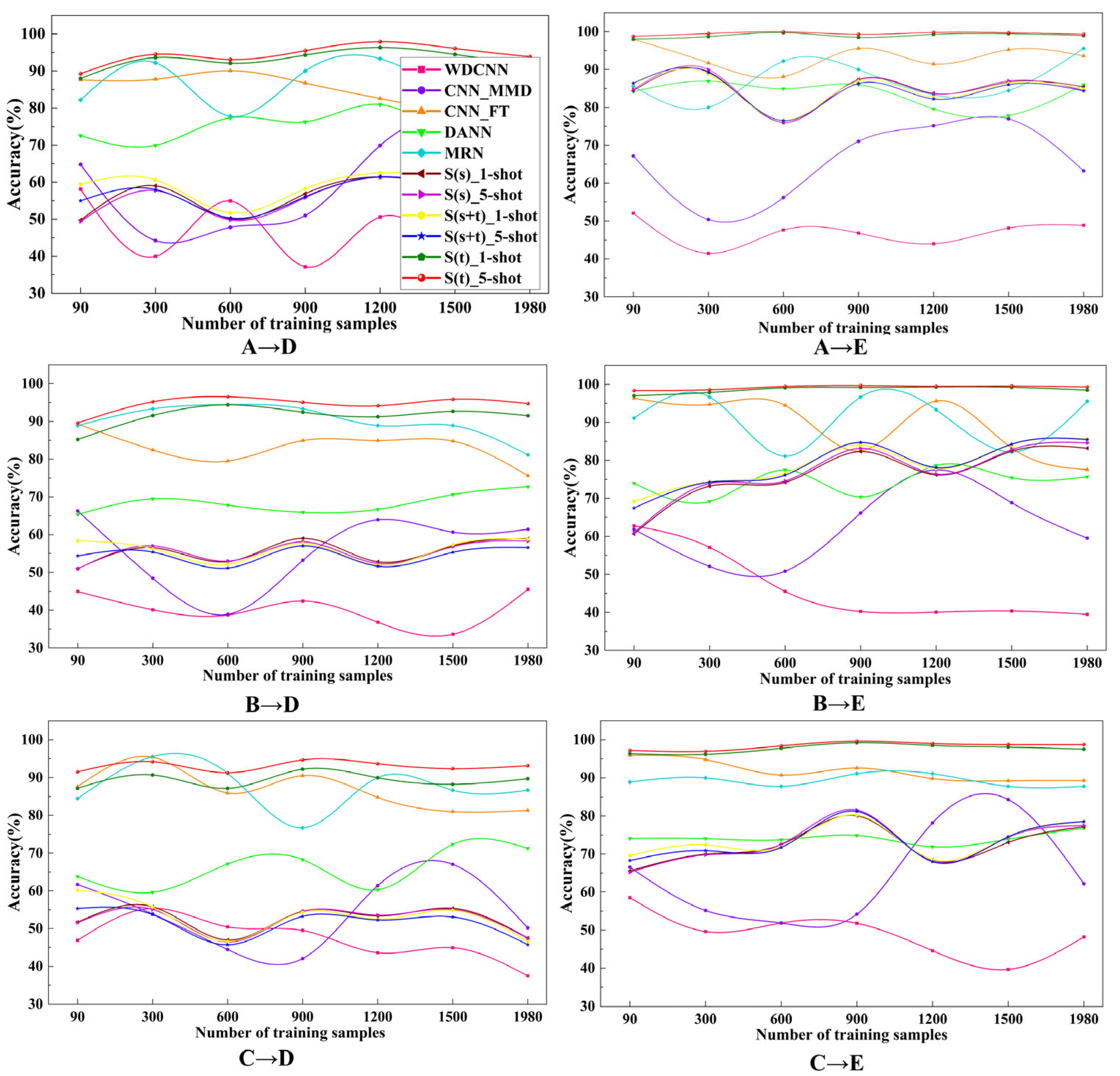
4.4. The Influence of Different Source Domain and the Number of Training Samples
5. Conclusions
- (1)
- With only a small amount of SNSASS, S(t) method greatly improves the accuracy of fault classification, and the accuracy of S(s+t) is not significantly improved, but increases with the increase in the number of SNSASS.
- (2)
- Compared with other methods, the proposed S(t) method has the highest accuracy in all cases and is also the most stable method.
- (3)
- S(t) can fully learn diagnostic knowledge in different source domains and sample numbers, and effectively use this knowledge to identify the health state of the target bearing, which has strong generalization and robustness. In addition, unlike the fine-tuning-based method, S(t) does not need secondary training, which is more convenient in some practical applications.
Author Contributions
Funding
Acknowledgments
Conflicts of Interest
References
- Zhang, S.; Zhang, S.; Wang, B.; Habetler, T.G. Deep Learning Algorithms for Bearing Fault Diagnostics—A Comprehensive Review. IEEE Access 2020, 8, 29857–29881. [Google Scholar] [CrossRef]
- Shi, H.; Fu, W.; Li, B.; Shao, K.; Yang, D. Intelligent Fault Identification for Rolling Bearings Fusing Average Refined Composite Multiscale Dispersion Entropy-Assisted Feature Extraction and SVM with Multi-Strategy Enhanced Swarm Optimization. Entropy 2021, 23, 527. [Google Scholar] [CrossRef] [PubMed]
- Liu, D.; Wang, Q.; Tao, J.; Li, G.; Wu, J. Fault Diagnosis Method Based on Improved Deep Boltzmann Machines. In Proceedings of the 2018 IEEE 7th Data Driven Control and Learning Systems Conference (DDCLS), Enshi, China, 25–27 May 2018; pp. 458–462. [Google Scholar]
- Zhao, B.; Zhang, X.; Li, H.; Yang, Z. Intelligent Fault Diagnosis of Rolling Bearings Based on Normalized CNN Considering Data Imbalance and Variable Working Conditions. Knowl.-Based Syst. 2020, 199, 105971. [Google Scholar] [CrossRef]
- Zhou, F.; Yang, S.; Fujita, H.; Chen, D.; Wen, C. Deep Learning Fault Diagnosis Method Based on Global Optimization GAN for Unbalanced Data. Knowl.-Based Syst. 2020, 187, 104837. [Google Scholar] [CrossRef]
- Wang, S.; Wang, D.; Kong, D.; Wang, J.; Li, W.; Zhou, S. Few-Shot Rolling Bearing Fault Diagnosis with Metric-Based Meta Learning. Sensors 2020, 20, 6437. [Google Scholar] [CrossRef]
- Wu, Z.; Lin, W.; Fu, B.; Guo, J.; Ji, Y.; Pecht, M. A Local Adaptive Minority Selection and Oversampling Method for Class-Imbalanced Fault Diagnostics in Industrial Systems. IEEE Trans. Reliab. 2020, 69, 1195–1206. [Google Scholar] [CrossRef]
- Zhang, Y.; Li, X.; Gao, L.; Wang, L.; Wen, L. Imbalanced Data Fault Diagnosis of Rotating Machinery Using Synthetic Oversampling and Feature Learning. J. Manuf. Syst. 2018, 48, 34–50. [Google Scholar] [CrossRef]
- Liu, Q.; Ma, G.; Cheng, C. Data Fusion Generative Adversarial Network for Multi-Class Imbalanced Fault Diagnosis of Rotating Machinery. IEEE Access 2020, 8, 70111–70124. [Google Scholar] [CrossRef]
- Soltanzadeh, P.; Hashemzadeh, M. RCSMOTE: Range-Controlled Synthetic Minority over-Sampling Technique for Handling the Class Imbalance Problem. Inf. Sci. 2021, 542, 92–111. [Google Scholar] [CrossRef]
- Zhang, K.; Chen, J.; Zhang, T.; He, S.; Pan, T.; Zhou, Z. Intelligent Fault Diagnosis of Mechanical Equipment under Varying Working Condition via Iterative Matching Network Augmented with Selective Signal Reuse Strategy. J. Manuf. Syst. 2020, 57, 400–415. [Google Scholar] [CrossRef]
- Fang, Q.; Wu, D. ANS-Net: Anti-Noise Siamese Network for Bearing Fault Diagnosis with a Few Data. Nonlinear Dyn. 2021, 104, 2497–2514. [Google Scholar] [CrossRef]
- Lu, N.; Hu, H.; Yin, T.; Lei, Y.; Wang, S. Transfer Relation Network for Fault Diagnosis of Rotating Machinery with Small Data. IEEE Trans. Cybern. 2021, 1–15. [Google Scholar] [CrossRef]
- Mai, S.; Hu, H.; Xu, J. Attentive Matching Network for Few-Shot Learning. Comput. Vis. Image Underst. 2019, 187, 102781. [Google Scholar] [CrossRef]
- Xiao, D.; Huang, Y.; Qin, C.; Liu, Z.; Li, Y.; Liu, C. Transfer Learning with Convolutional Neural Networks for Small Sample Size Problem in Machinery Fault Diagnosis. Proc. Inst. Mech. Eng. C J. Mech. Eng. Sci. 2019, 233, 5131–5143. [Google Scholar] [CrossRef]
- Zhang, T.; Chen, J.; Li, F.; Zhang, K.; Lv, H.; He, S.; Xu, E. Intelligent Fault Diagnosis of Machines with Small & Imbalanced Data: A State-of-the-Art Review and Possible Extensions. ISA Trans. 2021, 119, 152–171. [Google Scholar] [CrossRef]
- Ren, Z.; Zhu, Y.; Yan, K.; Chen, K.; Kang, W.; Yue, Y.; Gao, D. A Novel Model with the Ability of Few-Shot Learning and Quick Updating for Intelligent Fault Diagnosis. Mech. Syst. Signal Process. 2020, 138, 106608. [Google Scholar] [CrossRef]
- Zhang, A.; Li, S.; Cui, Y.; Yang, W.; Dong, R.; Hu, J. Limited Data Rolling Bearing Fault Diagnosis with Few-Shot Learning. IEEE Access 2019, 7, 110895–110904. [Google Scholar] [CrossRef]
- Li, X.; Jiang, H.; Zhao, K.; Wang, R. A Deep Transfer Nonnegativity-Constraint Sparse Autoencoder for Rolling Bearing Fault Diagnosis with Few Labeled Data. IEEE Access 2019, 7, 91216–91224. [Google Scholar] [CrossRef]
- Feng, Y.; Chen, J.; Zhang, T.; He, S.; Xu, E.; Zhou, Z. Semi-Supervised Meta-Learning Networks with Squeeze-and-Excitation Attention for Few-Shot Fault Diagnosis. ISA Trans. 2022, 120, 383–401. [Google Scholar] [CrossRef]
- Li, C.; Li, S.; Zhang, A.; He, Q.; Liao, Z.; Hu, J. Meta-Learning for Few-Shot Bearing Fault Diagnosis under Complex Working Conditions. Neurocomputing 2021, 439, 197–211. [Google Scholar] [CrossRef]
- Yu, C.; Ning, Y.; Qin, Y.; Su, W.; Zhao, X. Multi-Label Fault Diagnosis of Rolling Bearing Based on Meta-Learning. Neural Comput. Appl. 2021, 33, 5393–5407. [Google Scholar] [CrossRef]
- Wang, D.; Zhang, M.; Xu, Y.; Lu, W.; Yang, J.; Zhang, T. Metric-Based Meta-Learning Model for Few-Shot Fault Diagnosis under Multiple Limited Data Conditions. Mech. Syst. Signal Process. 2021, 155, 107510. [Google Scholar] [CrossRef]
- Pei, Z.; Jiang, H.; Li, X.; Zhang, J.; Liu, S. Data Augmentation for Rolling Bearing Fault Diagnosis Using an Enhanced Few-Shot Wasserstein Auto-Encoder with Meta-Learning. Meas. Sci. Technol. 2021, 32, 84007. [Google Scholar] [CrossRef]
- Zhang, S.; Ye, F.; Wang, B.; Habetler, T.G. Few-Shot Bearing Fault Diagnosis Based on Model-Agnostic Meta-Learning. IEEE Trans. Ind. Appl. 2021, 57, 4754–4764. [Google Scholar] [CrossRef]
- Feng, Y.; Chen, J.; Yang, Z.; Song, X.; Chang, Y.; He, S.; Xu, E.; Zhou, Z. Similarity-Based Meta-Learning Network with Adversarial Domain Adaptation for Cross-Domain Fault Identification. Knowl.-Based Syst. 2021, 217, 106829. [Google Scholar] [CrossRef]
- Wang, C.; Xu, Z. An Intelligent Fault Diagnosis Model Based on Deep Neural Network for Few-Shot Fault Diagnosis. Neurocomputing 2021, 456, 550–562. [Google Scholar] [CrossRef]
- He, Z.; Shao, H.; Wang, P.; Lin, J.; Cheng, J.; Yang, Y. Deep Transfer Multi-Wavelet Auto-Encoder for Intelligent Fault Diagnosis of Gearbox with Few Target Training Samples. Knowl.-Based Syst. 2020, 191, 105313. [Google Scholar] [CrossRef]
- Liu, Y.Z.; Shi, K.M.; Li, Z.X.; Ding, G.F.; Zou, Y.S. Transfer Learning Method for Bearing Fault Diagnosis Based on Fully Convolutional Conditional Wasserstein Adversarial Networks. Measurement 2021, 180, 109553. [Google Scholar] [CrossRef]
- Wu, J.; Zhao, Z.; Sun, C.; Yan, R.; Chen, X. Few-Shot Transfer Learning for Intelligent Fault Diagnosis of Machine. Measurement 2020, 166, 108202. [Google Scholar] [CrossRef]
- Yang, B.; Lei, Y.; Jia, F.; Xing, S. An Intelligent Fault Diagnosis Approach Based on Transfer Learning from Laboratory Bearings to Locomotive Bearings. Mech. Syst. Signal Process. 2019, 122, 692–706. [Google Scholar] [CrossRef]
- Guo, L.; Lei, Y.; Xing, S.; Yan, T.; Li, N. Deep Convolutional Transfer Learning Network: A New Method for Intelligent Fault Diagnosis of Machines with Unlabeled Data. IEEE Trans. Ind. Electron. 2019, 66, 7316–7325. [Google Scholar] [CrossRef]
- Zhang, W.; Peng, G.; Li, C.; Chen, Y.; Zhang, Z. A New Deep Learning Model for Fault Diagnosis with Good Anti-Noise and Domain Adaptation Ability on Raw Vibration Signals. Sensors 2017, 17, 425. [Google Scholar] [CrossRef] [PubMed]
- Case Western Reserve University Bearing Data Center Website. Available online: https://engineering.case.edu/bearingdatacenter/welcome (accessed on 8 July 2021).
- Lessmeier, C.; Kimotho, J.K.; Zimmer, D.; Sextro, W. Condition Monitoring of Bearing Damage in Electromechanical Drive Systems by Using Motor Current Signals of Electric Motors: A Benchmark Data Set for Data-Driven Classification. In Proceedings of the PHM Society European Conference 2016, Chengdu, China, 19–21 October 2016. [Google Scholar] [CrossRef]
- Xiao, D.; Huang, Y.; Zhao, L.; Qin, C.; Shi, H.; Liu, C. Domain Adaptive Motor Fault Diagnosis Using Deep Transfer Learning. IEEE Access 2019, 7, 80937–80949. [Google Scholar] [CrossRef]
- Li, F.; Chen, J.; Pan, J.; Pan, T. Cross-Domain Learning in Rotating Machinery Fault Diagnosis under Various Operating Conditions Based on Parameter Transfer. Meas. Sci. Technol. 2020, 31, 085104. [Google Scholar] [CrossRef]
- Ganin, Y.; Ustinova, E.; Ajakan, H.; Germain, P.; Larochelle, H.; Laviolette, F.; Marchand, M.; Lempitsky, V. Domain-Adversarial Training of Neural Networks. J. Mach. Learn. Res. 2016, 17, 1–35. [Google Scholar]
- Li, C.; Li, S.; Zhang, A.; Yang, L.; Zio, E.; Pecht, M.; Gryllias, K. A Siamese Hybrid Neural Network Framework for Few-Shot Fault Diagnosis of Fixed-Wing Unmanned Aerial Vehicles. J. Comput. Des. Eng. 2022, 9, 1511–1524. [Google Scholar] [CrossRef]


| No | Layer Type | Kernel Size/Stride | Kernel Number | Output Size (Width × Depth) | Padding |
|---|---|---|---|---|---|
| 1 | Conv1 | 64 × 1/16 × 1 | 16 | 128 × 16 | same |
| 2 | Pooling1 | 2 × 1/2 × 1 | 16 | 64 × 16 | valid |
| 3 | Conv2 | 3 × 1/1 × 1 | 32 | 64 × 32 | same |
| 4 | Pooling2 | 2 × 1/2 × 1 | 32 | 32 × 32 | valid |
| 5 | Conv3 | 3 × 1/1 × 1 | 64 | 32 × 64 | same |
| 6 | Pooling3 | 2 × 1/2 × 1 | 64 | 16 × 64 | valid |
| 7 | Conv4 | 3 × 1/1 × 1 | 64 | 16 × 64 | same |
| 8 | Pooling4 | 2 × 1/2 × 1 | 64 | 8 × 64 | valid |
| 9 | Conv5 | 3 × 1/1 × 1 | 64 | 6 × 64 | valid |
| 10 | Pooling5 | 2 × 1/2 × 1 | 64 | 3 × 64 | valid |
| 11 | Fully-connected | 100 | 1 | 100 × 1 |
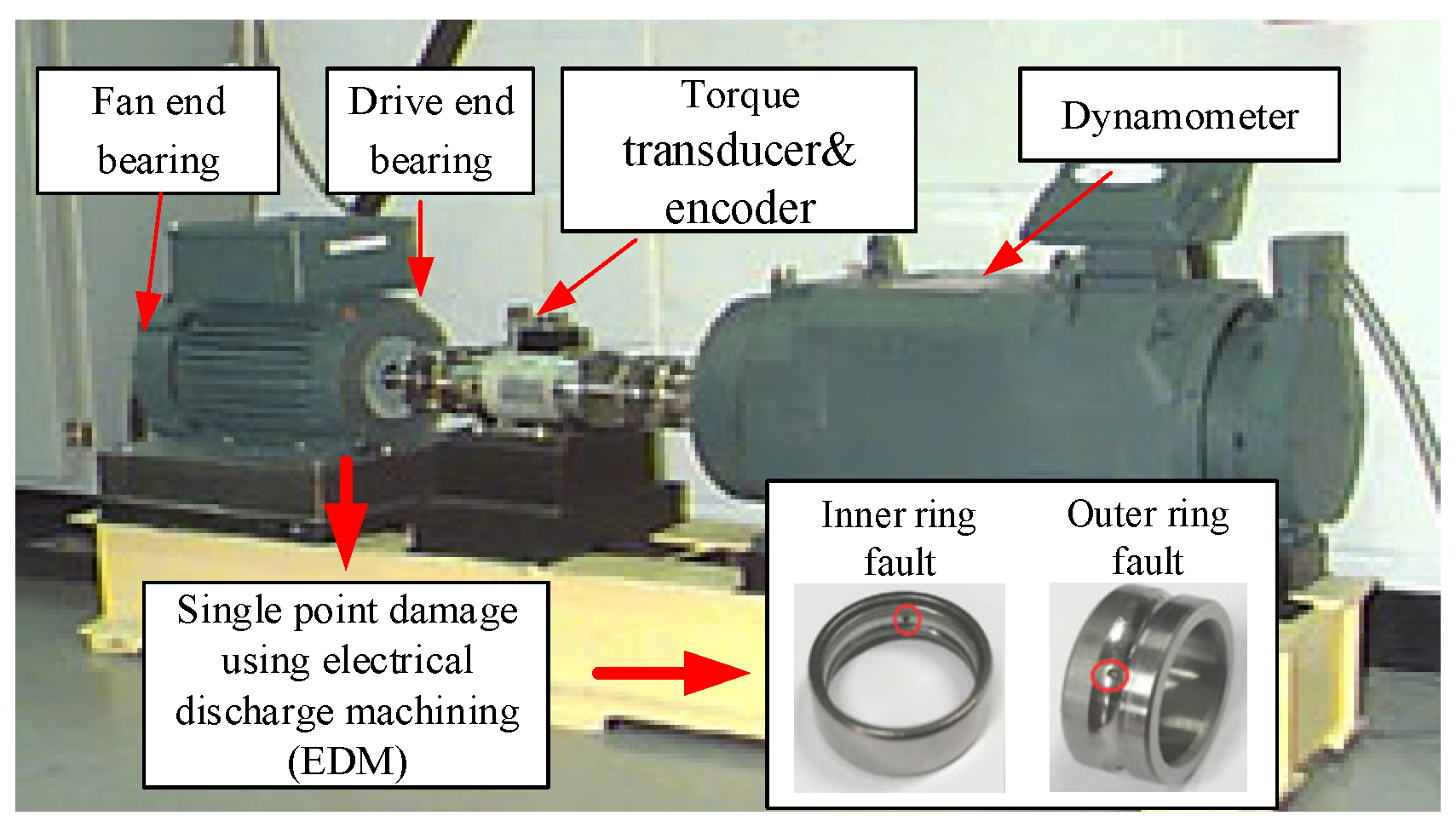
| Dataset Name | Name | Fault Location | Speed (rpm) | Loads (hp) |
|---|---|---|---|---|
| 0.021-OuterRace | Outer ring | 1772 | 1 | |
| A | 0.021-InnerRace | Inner ring | 1772 | 1 |
| Normal | None | 1772 | 1 | |
| 0.021-OuterRace | Outer ring | 1750 | 2 | |
| B | 0.021-InnerRace | Inner ring | 1750 | 2 |
| Normal | None | 1750 | 2 | |
| 0.021-OuterRace | Outer ring | 1730 | 3 | |
| C | 0.021-InnerRace | Inner ring | 1730 | 3 |
| Normal | None | 1730 | 3 |
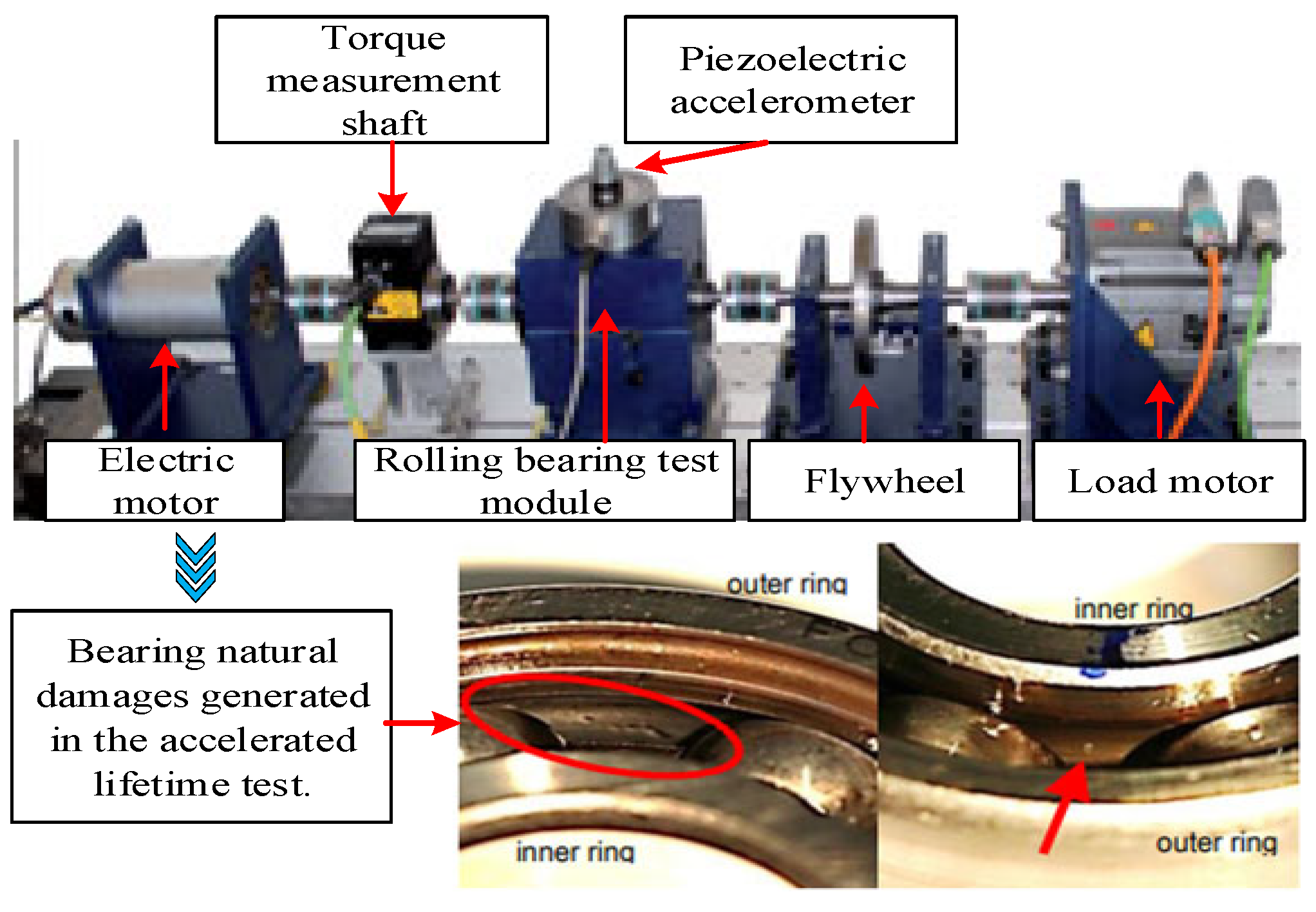
| Damage Level | Assigned Percentage Values | Limits for Bearing 6203 |
|---|---|---|
| 1 | 0–2% | ≤2 mm |
| 2 | 2–5% | >2 mm |
| Dataset Name | Name | Fault Location | Damage (Main Mode and Symptom) | Damage Level | Damage Feature | Load Torque (Nm) | Speed (rpm) | Radial Force (N) |
|---|---|---|---|---|---|---|---|---|
| D | KI04 | Inner ring | Fatigue: pitting | 1 | Single | 0.7 | 1500 | 1000 |
| KA04 | Outer ring | Fatigue: pitting | 1 | Single | 0.7 | 1500 | 1000 | |
| K005 | Normal | None | None | None | 0.7 | 1500 | 1000 | |
| E | KI16 | Inner ring | Fatigue: pitting | 2 | Single | 0.7 | 1500 | 1000 |
| KA16 | Outer ring | Fatigue: pitting | 2 | Single | 0.7 | 1500 | 1000 | |
| K004 | Normal | None | None | None | 0.7 | 1500 | 1000 |
| Sample Purpose | Inner Ring 0 | Outer Ring 1 | Normal 2 | Total | |
|---|---|---|---|---|---|
| Source domain | Training | 660 | 660 | 660 | 1980 |
| Target domain | SNSASS | 5 | 5 | 5 | 15 |
| Testing | 75 | 75 | 75 | 225 |
| Number | Experiment Name | Model | Support Set |
|---|---|---|---|
| 1 | S(s) | Siamese network | Training sample |
| 2 | S(s+t) | Siamese network | Training sample and SNSASS |
| 3 | S(t) | Siamese network | SNSASS |
Publisher’s Note: MDPI stays neutral with regard to jurisdictional claims in published maps and institutional affiliations. |
© 2022 by the authors. Licensee MDPI, Basel, Switzerland. This article is an open access article distributed under the terms and conditions of the Creative Commons Attribution (CC BY) license (https://creativecommons.org/licenses/by/4.0/).
Share and Cite
Zhang, Y.; Li, S.; Zhang, A.; Li, C.; Qiu, L. A Novel Bearing Fault Diagnosis Method Based on Few-Shot Transfer Learning across Different Datasets. Entropy 2022, 24, 1295. https://doi.org/10.3390/e24091295
Zhang Y, Li S, Zhang A, Li C, Qiu L. A Novel Bearing Fault Diagnosis Method Based on Few-Shot Transfer Learning across Different Datasets. Entropy. 2022; 24(9):1295. https://doi.org/10.3390/e24091295
Chicago/Turabian StyleZhang, Yizong, Shaobo Li, Ansi Zhang, Chuanjiang Li, and Ling Qiu. 2022. "A Novel Bearing Fault Diagnosis Method Based on Few-Shot Transfer Learning across Different Datasets" Entropy 24, no. 9: 1295. https://doi.org/10.3390/e24091295