Figure 1.
Random behaviors of the 4D-FDHNN chaotic system.
Figure 1.
Random behaviors of the 4D-FDHNN chaotic system.
Figure 2.
Phase diagrams of the 4D-FDHNN chaotic system for the initial value , fractional order , and step size (x-y plane; x-z plane; x-w plane; y-z plane; y-w plane; z-w plane).
Figure 2.
Phase diagrams of the 4D-FDHNN chaotic system for the initial value , fractional order , and step size (x-y plane; x-z plane; x-w plane; y-z plane; y-w plane; z-w plane).
Figure 3.
Attractor graph of the 4D-FDHNN chaotic system.
Figure 3.
Attractor graph of the 4D-FDHNN chaotic system.
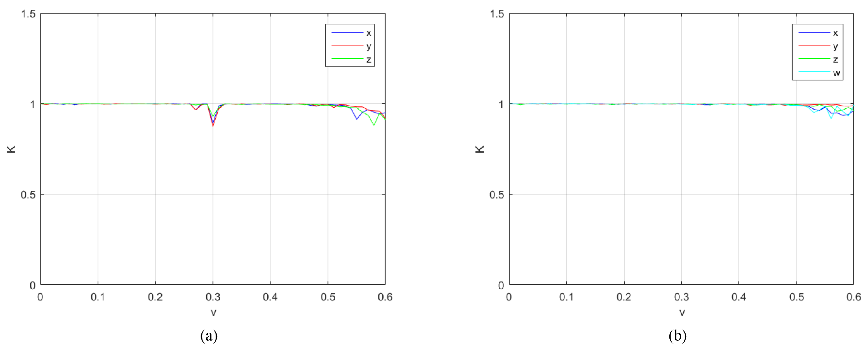
Figure 4.
0-1 test results. (a) the 0-1 test of 3D-FDHNN with ; (b) the 0-1 test of 4D-FDHNN with .
Figure 4.
0-1 test results. (a) the 0-1 test of 3D-FDHNN with ; (b) the 0-1 test of 4D-FDHNN with .
Figure 5.
0-1 test results. (a) the 0-1 test of 3D-FDHNN with ; (b) the 0-1 test of 4D-FDHNN with .
Figure 5.
0-1 test results. (a) the 0-1 test of 3D-FDHNN with ; (b) the 0-1 test of 4D-FDHNN with .
Figure 6.
Sample Entropy. (a) the sample entropy of 3D-FDHNN with ; (b) the sample entropy of 4D-FDHNN with .
Figure 6.
Sample Entropy. (a) the sample entropy of 3D-FDHNN with ; (b) the sample entropy of 4D-FDHNN with .
Figure 7.
Sample Entropy. (a) the sample entropy of 3D-FDHNN with ; (b) the sample entropy of 4D-FDHNN with .
Figure 7.
Sample Entropy. (a) the sample entropy of 3D-FDHNN with ; (b) the sample entropy of 4D-FDHNN with .
Figure 8.
Lyapunov exponent.
Figure 8.
Lyapunov exponent.
Figure 9.
Chaos game with three bases. (a) the first three iterations, (b) 1000 iterations, (c) 10,000 iterations.
Figure 9.
Chaos game with three bases. (a) the first three iterations, (b) 1000 iterations, (c) 10,000 iterations.
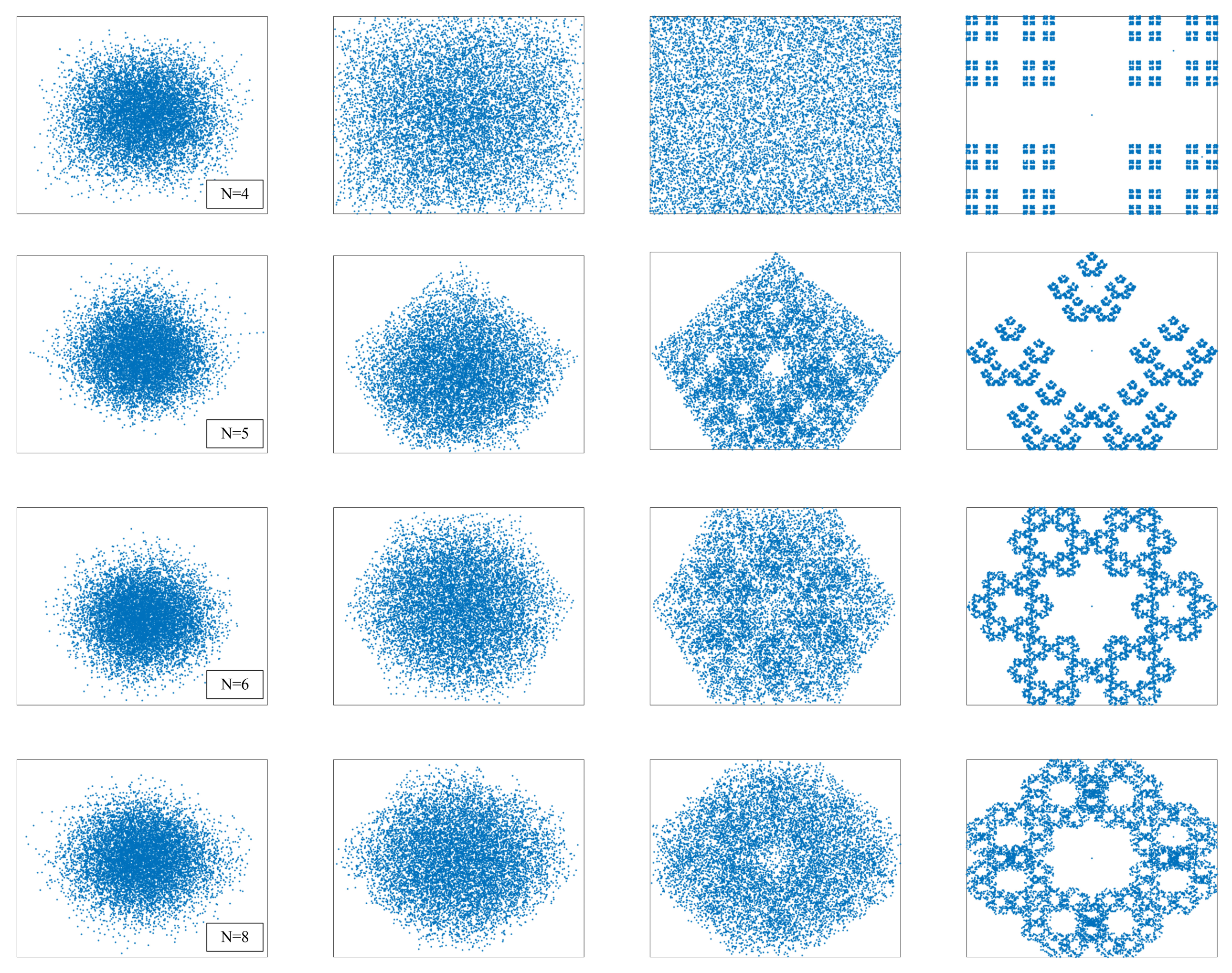
Figure 10.
Fractal iteration results under different parameters. (Each column from left to right is , , , and , respectively.).
Figure 10.
Fractal iteration results under different parameters. (Each column from left to right is , , , and , respectively.).
Figure 11.
Pixel matrix mapped in a two-dimensional rectangular coordinate system.
Figure 11.
Pixel matrix mapped in a two-dimensional rectangular coordinate system.
Figure 12.
Scrambling effects of a fractal-like model. (a) original image “boat” (); (b) original image “airfield” (); (c) scrambled of (a); (d) scrambled of (b).
Figure 12.
Scrambling effects of a fractal-like model. (a) original image “boat” (); (b) original image “airfield” (); (c) scrambled of (a); (d) scrambled of (b).
Figure 13.
Encryption process.
Figure 13.
Encryption process.
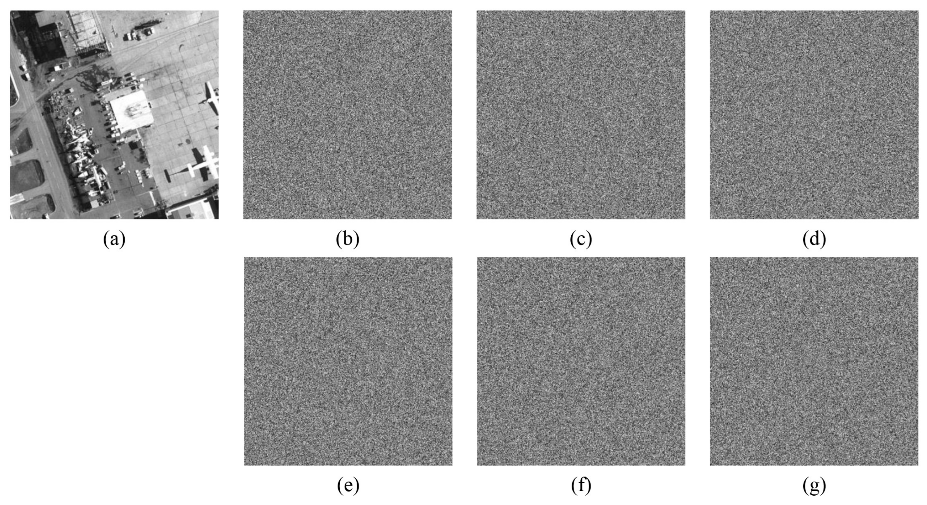
Figure 14.
Comparison of scrambling effects. (a) original image “airfield”; (b) only row-column dual scrambling; (c) only fractal-like model scrambling; (d) combined scrambling (proposed).
Figure 14.
Comparison of scrambling effects. (a) original image “airfield”; (b) only row-column dual scrambling; (c) only fractal-like model scrambling; (d) combined scrambling (proposed).
Figure 15.
Hilbert curve of order 1–5.
Figure 15.
Hilbert curve of order 1–5.
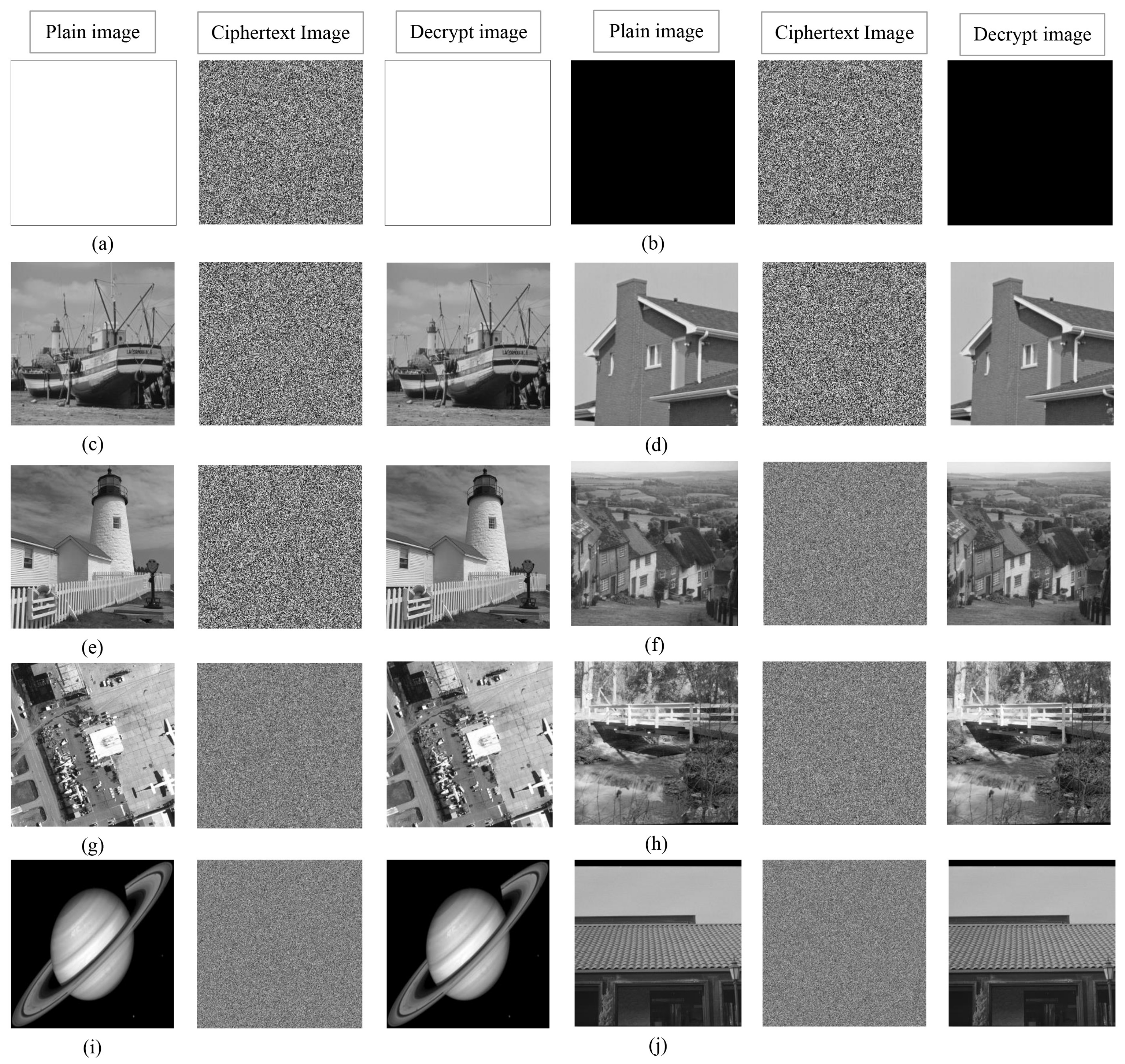
Figure 16.
Encryption and decryption effects. (a–e) show the images with size of : “boat256”, “house256”, “kod256”, “all-white”, “all-black”. (f–h) are the images with size of : “hill512”, “airfield512”, “bridge512”. (i,j) are the images with the size of : “saturn1024”, “tile roof1024”.
Figure 16.
Encryption and decryption effects. (a–e) show the images with size of : “boat256”, “house256”, “kod256”, “all-white”, “all-black”. (f–h) are the images with size of : “hill512”, “airfield512”, “bridge512”. (i,j) are the images with the size of : “saturn1024”, “tile roof1024”.
Figure 17.
Key sensitivity of “boat256”. (a) The decrypted image with correct key; (b) the decrypted image with key ; (c) the decrypted image with key ; (d) the decrypted image with key ; (e) the decrypted image with key ; (f) the decrypted image with key ; (g) the decrypted image with key .
Figure 17.
Key sensitivity of “boat256”. (a) The decrypted image with correct key; (b) the decrypted image with key ; (c) the decrypted image with key ; (d) the decrypted image with key ; (e) the decrypted image with key ; (f) the decrypted image with key ; (g) the decrypted image with key .
Figure 18.
Key sensitivity of “airfield512”. (a) the decrypted image with a correct key; (b) the decrypted image with key ; (c) the decrypted image with key ; (d) the decrypted image with key ; (e) the decrypted image with key ; (f) the decrypted image with key ; (g) the decrypted image with key .
Figure 18.
Key sensitivity of “airfield512”. (a) the decrypted image with a correct key; (b) the decrypted image with key ; (c) the decrypted image with key ; (d) the decrypted image with key ; (e) the decrypted image with key ; (f) the decrypted image with key ; (g) the decrypted image with key .
Figure 19.
Key sensitivity of “saturn1024”. (a) the decrypted image with correct key; (b) the decrypted image with key ; (c) the decrypted image with key ; (d) the decrypted image with key ; (e) the decrypted image with key ; (f) the decrypted image with key ; (g) the decrypted image with key .
Figure 19.
Key sensitivity of “saturn1024”. (a) the decrypted image with correct key; (b) the decrypted image with key ; (c) the decrypted image with key ; (d) the decrypted image with key ; (e) the decrypted image with key ; (f) the decrypted image with key ; (g) the decrypted image with key .
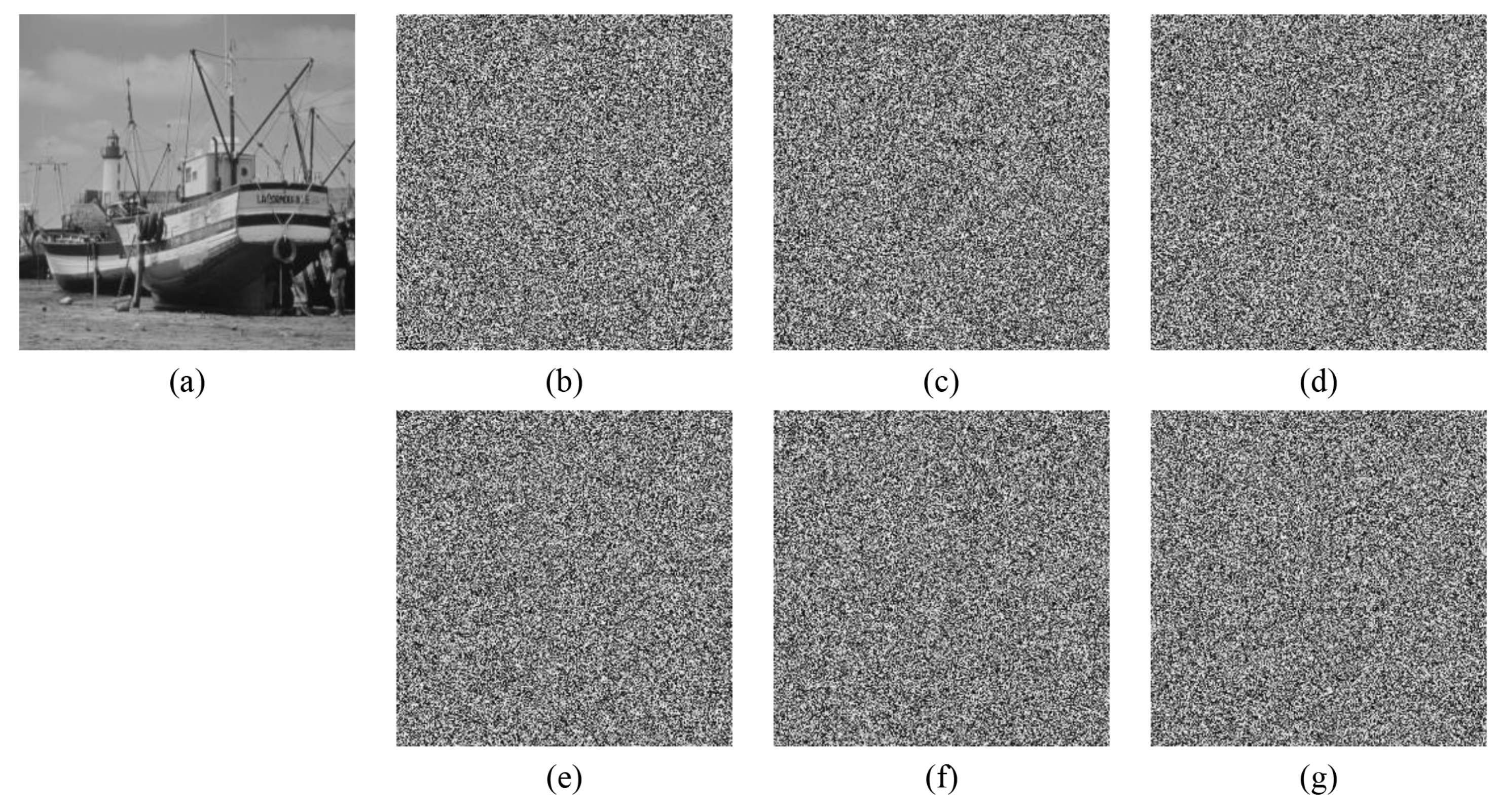
Figure 20.
The difference between ciphertext images when the key changes slightly. (a) plain image “boat256”; (b) ciphertext Images with ; (c) ciphertext Images with ; (d) the differences between (b,c); (e) plain image “airfield512”; (f) ciphertext Images with ; (g) ciphertext images with ; (h) the differences between (f,g); (i) plain image “saturn1024”; (j) ciphertext Images with ; (k) ciphertext images with ; (l) the differences between (j,k).
Figure 21.
Histograms of plain images and their corresponding cipher images. Each plain image is followed by its histogram, the corresponding cipher image, and its histogram.
Figure 21.
Histograms of plain images and their corresponding cipher images. Each plain image is followed by its histogram, the corresponding cipher image, and its histogram.
Figure 22.
Adjacent pixel correlation of “boat256”. (a) plain image “boat256”; (b–d) correlation of adjacent pixels in the horizontal, vertical, and diagonal directions of (a); (e) ciphertext image of (a); (f–h) correlation of adjacent pixels in the horizontal, vertical, and diagonal directions of (e).
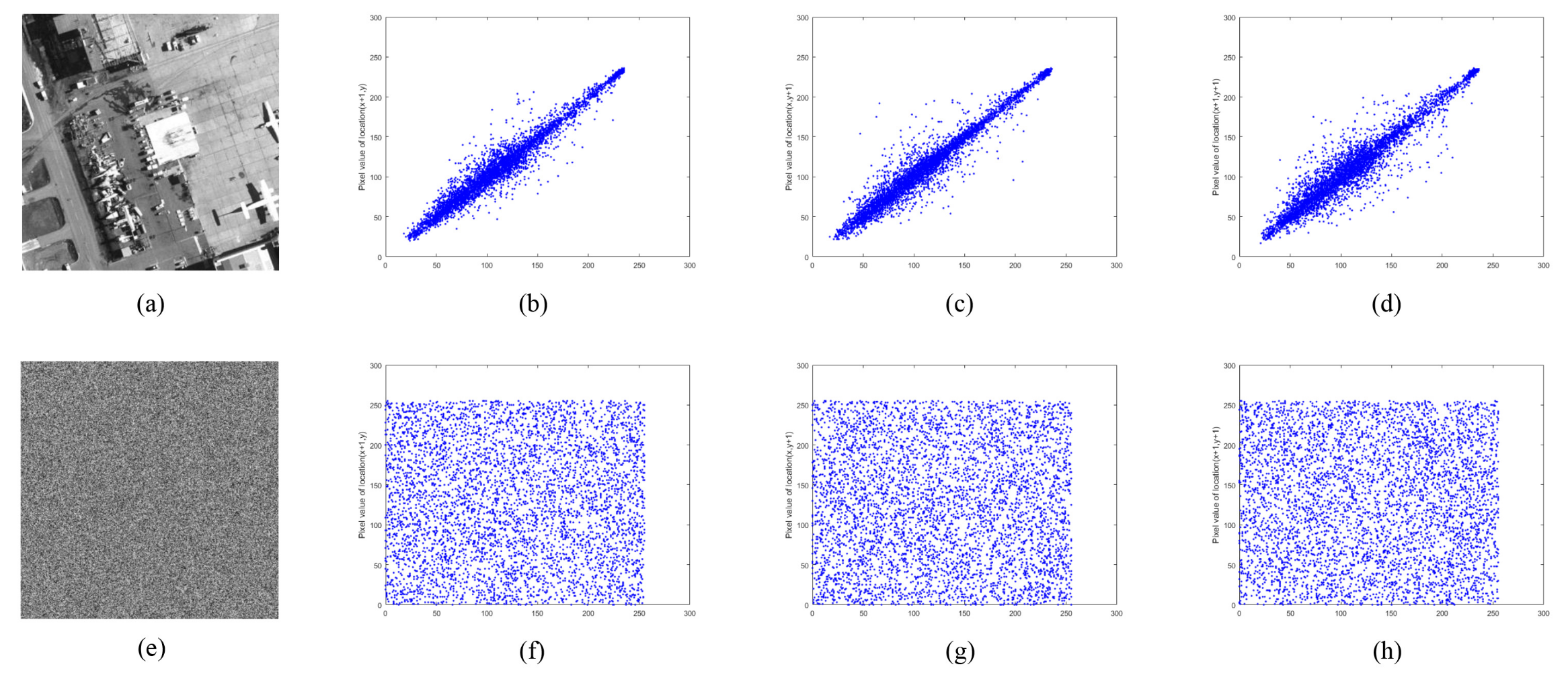
Figure 23.
Adjacent pixel correlation of “airfield512”. (a) plain image “airfield512”; (b–d) correlation of adjacent pixels in the horizontal, vertical, and diagonal directions of (a); (e) ciphertext image of (a). (f–h) correlation of adjacent pixels in the horizontal, vertical, and diagonal directions of (e).
Figure 24.
Adjacent pixel correlation of “saturn1024”. (a) plain image “saturn1024”; (b–d) correlation of adjacent pixels in the horizontal, vertical, and diagonal directions of (a); (e) ciphertext image of (a); (f–h) correlation of adjacent pixels in the horizontal, vertical, and diagonal directions of (e).
Figure 25.
Salt and Pepper noise test of “boat256”. The first row from left to right: encrypted image with 0.5%, 1%, 5%, 10% and 20% Salt and Pepper noise added. The second row: decrypted image of the corresponding cipher image in the first row.
Figure 25.
Salt and Pepper noise test of “boat256”. The first row from left to right: encrypted image with 0.5%, 1%, 5%, 10% and 20% Salt and Pepper noise added. The second row: decrypted image of the corresponding cipher image in the first row.
Figure 26.
Salt and Pepper noise test of “airfield512”. The first row from left to right: encrypted image with 0.5%, 1%, 5%, 10% and 20% Salt and Pepper noise added. The second row: decrypted image of the corresponding cipher image in the first row.
Figure 26.
Salt and Pepper noise test of “airfield512”. The first row from left to right: encrypted image with 0.5%, 1%, 5%, 10% and 20% Salt and Pepper noise added. The second row: decrypted image of the corresponding cipher image in the first row.
Figure 27.
Salt and Pepper noise test of “saturn1024”. The first row from left to right: encrypted image with 0.5%, 1%, 5%, 10%, and 20% Salt and Pepper noise added. The second row: decrypted image of the corresponding cipher image in the first row.
Figure 27.
Salt and Pepper noise test of “saturn1024”. The first row from left to right: encrypted image with 0.5%, 1%, 5%, 10%, and 20% Salt and Pepper noise added. The second row: decrypted image of the corresponding cipher image in the first row.
Figure 28.
Gaussian noise test of “airfield512”. The first row from left to right: encrypted image with 0.1%, 0.5%, 1%, 5%, and 10% Gaussian noise added. The second row: decrypted image of the corresponding cipher image in the first row.
Figure 28.
Gaussian noise test of “airfield512”. The first row from left to right: encrypted image with 0.1%, 0.5%, 1%, 5%, and 10% Gaussian noise added. The second row: decrypted image of the corresponding cipher image in the first row.
Figure 29.
Clipping attack test of “airfield512”. The first row from left to right: encrypted image has been clipped 1/16, 1/8, 1/4, 1/4 (middle), and 1/2. The second row: decrypted image of the corresponding cipher image in the first row.
Figure 29.
Clipping attack test of “airfield512”. The first row from left to right: encrypted image has been clipped 1/16, 1/8, 1/4, 1/4 (middle), and 1/2. The second row: decrypted image of the corresponding cipher image in the first row.
Table 1.
The key point of Lyapunov exponent turning into positive.
Table 1.
The key point of Lyapunov exponent turning into positive.
| h | Lyapunov Exponent |
|---|
| | | |
|---|
| 0.84 | −0.0211 | −0.0078 | −0.0561 | −0.0022 |
| 0.85 | −0.0094 | 0.0090 | −0.0493 | 0.0177 |
| 0.86 | 0.00791 | 0.0330 | 0.0311 | −0.0020 |
| 0.87 | 0.03733 | −0.0059 | −0.0027 | 0.0390 |
| 0.88 | 0.06598 | 0.0038 | 0.0751 | 0.0113 |
Table 2.
NIST randomness tests for the proposed scheme and its comparison.
Table 2.
NIST randomness tests for the proposed scheme and its comparison.
| Image Size | | | |
|---|
|
Tests
| p-Value
|
Result
| p-Value
|
Result
| p-Value
|
Result
|
|---|
| Approximate Entropy | 0.921541 | ✓ | 0.948753 | ✓ | 0.85384 | ✓ |
| Block Frequency | 0.821153 | ✓ | 0.618297 | ✓ | 0.996283 | ✓ |
| Cumulative Sums | 0.42738 | ✓ | 0.023076 | ✓ | 0.125491 | ✓ |
| FFT | 0.705674 | ✓ | 0.552252 | ✓ | 0.196993 | ✓ |
| Frequency | 0.33783 | ✓ | 0.022113 | ✓ | 0.258306 | ✓ |
| Linear Complexity | 0.042136 | ✓ | 0.367285 | ✓ | 0.676756 | ✓ |
| Longest Runs of 1 s | 0.860484 | ✓ | 0.07015 | ✓ | 0.927182 | ✓ |
| Non-overlapping Templates | 0.500097 | ✓ | 0.353505 | ✓ | 0.351968 | ✓ |
| Overlapping Templates | 0.370476 | ✓ | 0.819045 | ✓ | 0.16745 | ✓ |
| Random Excursions | 0.841748 | ✓ | 0.050996 | ✓ | 0.140009 | ✓ |
| Random Excursions Variant | 0.101973 | ✓ | 0.589966 | ✓ | 0.340509 | ✓ |
| Rank | 0.615691 | ✓ | 0.727356 | ✓ | 0.036279 | ✓ |
| Runs | 0.858687 | ✓ | 0.561305 | ✓ | 0.853917 | ✓ |
| Serial | 0.283802 | ✓ | 0.403982 | ✓ | 0.70536 | ✓ |
| Universal | 0.806738 | ✓ | 0.698998 | ✓ | 0.259228 | ✓ |
Table 3.
Correlation coefficients between adjacent pixels of the image.
Table 3.
Correlation coefficients between adjacent pixels of the image.
| Image | Direction | Plain Image | Cipher Image |
|---|
| boat256 | | 0.9546 | −0.0198 |
| | | 0.9416 | 0.0046 |
| | | 0.9074 | −0.0026 |
| house256 | | 0.9686 | 0.0082 |
| | | 0.9773 | 0.0001 |
| | | 0.9514 | −0.0221 |
| kod256 | | 0.9127 | 0.0002 |
| | | 0.8748 | 0.0005 |
| | | 0.8016 | 0.0179 |
| hill512 | | 0.9737 | 0.0087 |
| | | 0.9710 | −0.0008 |
| | | 0.9520 | 0.0046 |
| airfield512 | | 0.9412 | −0.0007 |
| | | 0.9421 | −0.0060 |
| | | 0.9059 | 0.0077 |
| bridge512 | | 0.9229 | −0.0078 |
| | | 0.9413 | 0.0059 |
| | | 0.8932 | 0.0014 |
| saturn1024 | | 0.9731 | 0.0024 |
| | | 0.9900 | −0.0001 |
| | | 0.9669 | 0.0012 |
| tile roof1024 | | 0.9996 | −0.0007 |
| | | 0.9995 | 0.0000 |
| | | 0.9987 | −0.0035 |
| Ref. [29] | | 0.8364 | 0.0069 |
| | | 0.8848 | 0.0037 |
| | | 0.8690 | −0.0079 |
| Ref. [35] | | 0.9356 | 0.0236 |
| | | 0.9604 | 0.0235 |
| | | 0.9116 | 0.0189 |
Table 4.
Information entropy.
Table 4.
Information entropy.
| Algorithm | Image | Information Entropy |
|---|
| Proposed | boat256 | 7.9970 |
| | house256 | 7.9970 |
| | kod256 | 7.9964 |
| | all-white | 7.9975 |
| | all-black | 7.9975 |
| | hill512 | 7.9994 |
| | bridge512 | 7.9992 |
| | airfield512 | 7.9992 |
| | saturn1024 | 7.9998 |
| | tile roof1024 | 7.9998 |
| Ref. [38] | | 7.9899 |
| | | 7.9914 |
| | | 7.9919 |
| Ref. [39] | | 7.9975 |
Table 5.
Plain image sensitivity analysis.
Table 5.
Plain image sensitivity analysis.
| Algorithm | NPCR | UACI |
|---|
| Proposed-boat256 | 99.6109 | 33.4645 |
| Proposed-airfield512 | 99.6048 | 33.4054 |
| Proposed-saturn1024 | 99.6036 | 33.4606 |
| Ref. [35]- | 99.6277 | 33.5045 |
| Ref. [35]- | 99.6025 | 33.4814 |
| Ref. [35]- | 99.6233 | 33.4678 |
| Ref. [38]- | 99.6002 | 33.5524 |
| Ref. [38]- | 99.5937 | 33.4086 |
| Ref. [38]- | 99.5991 | 33.4656 |
| Ref. [42] | 98.9874 | 33.2516 |
Table 6.
PSNR and MSE results.
Table 6.
PSNR and MSE results.
| Index | MSE | PSNR |
|---|
| boat256 | 7697.5205 | 9.2673 |
| airfield512 | 9310.7735 | 8.4409 |
| saturn1024 | 15,142.9713 | 6.3287 |
Table 7.
Running time analysis.
Table 7.
Running time analysis.
| Algorithm | Image Size | Running Time (s) |
|---|
| Proposed-boat256 | | 0.0806 |
| Proposed-house256 | | 0.0757 |
| Proposed-kod256 | | 0.0774 |
| Proposed-hill512 | | 0.3395 |
| Proposed-airfield512 | | 0.3494 |
| Proposed-bridge512 | | 0.3203 |
| Proposed-saturn1024 | | 1.3284 |
| Proposed-tile roof1024 | | 1.3175 |
| | | 3.3833 |
| Ref. [29] | | 0.4060 |
| Ref. [32] | | 0.8158 |
| Ref. [38] | | 0.459837 |
| | | 1.769703 |
| | | 2.700164 |
| Ref. [45] | | 0.7738 |
| Ref. [46] | | 0.256722 |
| | | 0.620413 |
| | | 2.895086 |


