
Grand Canonical Ensembles of Sparse Networks and Bayesian Inference


1
School of Mathematical Sciences, Queen Mary University of London, London E1 4NS, UK
2
The Alan Turing Institute, The British Library, London NW1 2DB, UK
Entropy 2022, 24(5), 633; https://doi.org/10.3390/e24050633
Submission received: 13 April 2022
/
Revised: 25 April 2022
/
Accepted: 27 April 2022
/
Published: 30 April 2022
(This article belongs to the Topic Complex Systems and Network Science)
Abstract
:Maximum entropy network ensembles have been very successful in modelling sparse network topologies and in solving challenging inference problems. However the sparse maximum entropy network models proposed so far have fixed number of nodes and are typically not exchangeable. Here we consider hierarchical models for exchangeable networks in the sparse limit, i.e., with the total number of links scaling linearly with the total number of nodes. The approach is grand canonical, i.e., the number of nodes of the network is not fixed a priori: it is finite but can be arbitrarily large. In this way the grand canonical network ensembles circumvent the difficulties in treating infinite sparse exchangeable networks which according to the Aldous-Hoover theorem must vanish. The approach can treat networks with given degree distribution or networks with given distribution of latent variables. When only a subgraph induced by a subset of nodes is known, this model allows a Bayesian estimation of the network size and the degree sequence (or the sequence of latent variables) of the entire network which can be used for network reconstruction.
1. Introduction
Networks [1,2] have the ability to capture the topology of complex systems ranging from the brain to financial networks. Network models are key to have reliable unbiased null models of the network and to explain emergent phenomena of network evolution. Network model can be classified in two major classes: equilibrium maximum entropy models [3,4,5,6,7,8,9,10,11,12,13,14,15] and growing network models [1,16,17,18]. While growing network models have a number of nodes that increases in time, maximum entropy models are used so far only for treating networks of a given number of nodes N. In this paper we are interested in extending the realm of maximum entropy network models to networks of varying network size N.
Maximum entropy network ensembles are the least biased ensembles satisfying a given set of constraints. As such maximum entropy ensembles are widely used as null models and for network reconstruction starting from features associated to the nodes of the network. Given the profound relation between information theory and statistical mechanics [19,20], maximum entropy network ensembles can be distinguished between microcanonical ensembles and canonical ensembles [3,21,22] similarly to the analogous distinction traditionally introduced in statistical mechanics for ensembles of particles. Microcanonical network ensembles are ensembles of networks of N nodes satisfying some hard constraints (such as the total number of links, or the given degree sequence). Canonical network ensembles instead are ensembles of networks of N nodes satisfying some soft constraints, (such as the expected total number of links or the expected degree sequence). The canonical ensembles with expected degree sequence can be also formulated as latent variable models where the latent variables can be associated to the nodes [5,23].
Maximum entropy models have been very successful in solving challenging inference models [6,8,24,25,26], however they have the limitation that they only treat networks with a given fixed number of nodes N. Indeed in several scenarios, the number of nodes might not be fixed or might not be known. In this context an important problem is to compare networks of different network sizes. For instance in brain imaging one might choose a finer grid or a coarser grid of brain regions and an outstanding problem in machine learning is how to build neural networks that can generalize well when tested on network data with different network size than the network data in the training set [27,28].
In order to have network ensembles that can treat networks of different size, here we introduce the grand canonical network ensembles in which the number of nodes can vary. A well-defined grand-canonical network ensemble necessarily needs to be exchangeable [29], i.e., needs to be invariant under permutation of labels of the nodes of the network, so that removing or adding a node has an effect that is independent of the particular choice of the node added or removed.
The research on exchangeable networks is currently very vibrant. The graphon model [30] is the most well established exchangeable network model. However this model is dense, i.e., the number of links scales quadratically with the number of nodes while the vast majority of the network data is sparse with a total number of links scaling linearly with the network size. In other words most of the real world networks have constant average degree. However popular models for sparse networks such as the configuration model [31] and the exponential random graphs [4] are not exchangeable. In fact these models treat networks of labelled nodes with given degree or with given expected degree sequence. Therefore the network ensemble is not invariant under permutation of the node labels, except if all the degrees of all the expected degrees of the network are the same (for a more diffused discussion of why these networks are not exchangeable see discussion in ref. [32]). Several works have been proposed exchangeable network models in the when the average degree of the network diverges sublinearly with the network size [33,34,35,36,37,38]. Only recently, in ref. [32], a framework able to model sparse exchangeable networks in the limit of constant degree, has been proposed. The model is very general and has been extended to treat generalized network structures including multiplex networks [39] and simplicial complexes [40]. However the model is well defined only for finite networks of large but finite number of nodes N as exchangeable sparse networks need to obey the Aldous-Hoover theorem [41,42] according to which infinite sparse exchangeable networks must vanish. An alternative strategy for formulating exchangeable ensembles is to consider ensembles of unlabelled networks for which several results are already available [43].
Here we build on the recently proposed exchangeable sparse network ensembles [32] to formulate hierarchical grand-canonical ensembles of sparse networks. The proposed grand-canonical ensembles are hierarchical models [25,44] with variable number of nodes N and with given degree distribution or alternatively given latent variable distributions. The grand canonical approach provides a way to circumvent the limitations imposed by the Aldous-Hoover theorem because in this framework one considers a mixture of network ensembles with finite but unspecified and arbitrary large network sizes. In this paper we define the grand-canonical ensembles and we characterize them with statistical mechanics methods, evaluating their entropy, the marginal probability of a link and proposing generative algorithms to sample networks from these ensembles. [Note that the proposed grand canonical ensembles differ from the ensembles proposed in refs. [45,46], as in our case we consider networks with undetermined number of nodes, while in refs. [45,46] is the total sum of weights of weighted networks that is allowed to vary. From the statistical mechanics perspective our approach is fully classical while in refs. [45,46] networks ensembles are treated as quantum mechanical ensembles where the particles are associated to the links of the network and the adjacency matrix elements play the role of occupation numbers.].
Finally, we use the gran-canonical network ensembles to solve an inference problem. We consider a scenario in which the entire network has an unknown number of nodes, and we have only access to a subgraph induced by a subset of its nodes. In this hypothesis we use the grand-canonical network models to perform a Bayesian estimation of the true parameters of the network model (given by the network size and the degree sequence or the sequence of latent variables). This a posteriori estimate of the parameters can then be used to reconstruct the unknown part of the network.
2. The Grand Canonical Network Ensemble with Given Degree Distribution
We consider the hierarchical grand canonical ensemble of exchangeable sparse simple networks where we associate to every network with nodes the probability
where indicates the probability that the network G has N nodes, indicates the conditional probability that the network has degree sequence given that the network has N nodes, and indicates the probability of the network G with adjacency matrix given that the network has N nodes and degree sequence (see Figure 1 for a schematic representation of the model).
To be specific we consider the following model giving rise to the hierarchical grand canonical ensemble of exchangeable simple models:
- (1)
- Drawing the total number of nodes N of the network. Let us discuss suitable choices for the distribution of the number of nodes N with N greater or equal than some minimum number of nodes . We indicate the distribution asWhile a statistical mechanics approach would suggest to take a distribution with a well defined mean value (such as the exponential distribution)where C is a normalization constant and , in the context of network science it might actually be relevant to consider also broad distributions such as power-law distributionswhere D is a normalization constant and .
- (2)
- Drawing the degree sequence of the network. In order to obtain a sparse exchangeable network ensemble with given degree distribution having finite average degree , minimum allowed degree and maximum allowed degree K we consider the following expression for the probability of a given degree sequence given the total number of nodeswhere indicates the Heaviside function if and otherwise and where we used the notation . In the following we will indicate with L the total number of links of the network given by . Note that is independent of the labels of the nodes, i.e., all the degree sequences that can be obtained by a permutation of the node labels of a given degree sequence have the same probability .
- (3)
- Drawing the adjacency matrix of the network. The probability of a network G with adjacency matrix given the total number of nodes N of the network and the degree sequence is chosen in the least biased way by drawing the network from a uniform distribution, i.e., the conditional probability is equivalent to the probability of a network in the microcanonical ensemble. Therefore, by indicating with the total number of networks with N nodes and degree sequence and with the entropy of the ensemble we can express as
It follows that the hierarchical grand canonical ensemble for exchangeable sparse networks can be cast into an Hamiltonian ensemble with probability given by
with Hamiltonian given by
This Hamiltonian is global and is invariant under permutation of the node labels, therefore this hierarchical grand canonical ensemble is exchangeable. Indeed we have that the probability of a network given by Equation (8) obeys
where is any network obtained from network G under a generic permutation of the labels of the nodes. Moreover we note that for , i.e., when the network size is fixed this model reduces to the exchangeable model for sparse network ensemble proposed in ref. [32].
3. The Grand Canonical Network Ensemble with Given Distribution of the Latent Variables
The grand canonical formalism can also be easily extended to treat network models with latent variables associated to the nodes of the network . Note that here and in the following we assume that the latent variables take discrete values. To this end we can consider the soft grand canonical hierarchical model associating to each network with nodes, latent variables and adjacency matrix the probability
with
where is an arbitrary prior on the number of nodes in the network defined for . Typical examples of the distribution are given by Equations (3) and (4). The probability of the latent variables is chosen to be exchangeable and given by
where is the probability distribution of each latent variable. The distribution can be chosen arbitrarily, as long as the expectation of is finite. The probability of the network given the network size and the latent variables is chosen to be derived by a Bernoulli variable for each link, with probability of observing a link between node i and node j conditioned on the value of their latent variables given by , i.e.,
To be concrete we consider the following expression for the probability which is the general expression of the marginal probability of a link in canonical network ensembles (or equivalently exponential random graph models),
The advantage of taking this expression for the probability is that is always smaller or equal to one for every value of the latent variables. Therefore in this model we do not need to impose a structural cutoff on the latent variables. In summary the grand canonical network ensemble with given latent variable distribution is a hierarchical network model in which given the network size and latent variables the network is drawn according to a canonical ensemble of networks. In this ensemble the probability of a network G can be written in Hamiltonian form as
with Hamiltonian given by
This Hamitonian is invariant under permutation of the node labels, therefore this model is exchangeable.
4. The Entropy of Grand Canonical Ensembles
In this paragraph we show that the entropy S [3,48] of the two proposed grand canonical network ensembles, defined as
can be decomposed into contributions that reflect the uncertainty related to an increasing number of hierarchical levels of the model. In order to show this results we discuss separately the entropy of the two proposed grand canonical ensembles.
4.1. Entropy of the Grand Canonical Ensemble with Given Degree Distribution
The entropy S of the ensemble fixing the degree distribution can be decomposed into the entropy of the model at different levels of the hierarchy according to the following expression,
where is the entropy associated to the number of typical choices of the total number of nodes N, is the entropy associated to the choice of the degree sequence averaged over the distribution and is the average of the Gibbs entropy [3] of the networks with given degree sequence averaged over the distribution and . In other words we have
4.2. Entropy of the Grand Canonical Ensemble with Given Latent Variable Distribution
Similarly to the previous case, it is easy to show that the entropy of the ensemble fixing the distribution of the latent variables can be decomposed into the entropy of the model at different levels of their hierarchy, according to the following expression
where is the entropy associated to the number of typical choices of the total number of nodes N, is the entropy associated to the choice of the latent variable distribution averaged over the distribution and is the average of the Shannon entropy [3] of the networks with given sequence of latent variables averaged over the distribution and . In other words we have
where the Shannon entropy of the network given the sequence of latent variables and the network size N can be expressed as
5. Marginal Probability of a Link
5.1. The Case of the Grand Canonical Ensemble with Given Degree Distribution
The grand canonical ensemble of exchangeable sparse network ensembles is an ensemble in which the total number of nodes is not specified. If we consider the networks of this ensemble having a given number of nodes N, the model reduces to the exchangeable sparse network ensemble proposed in ref. [32] whose marginal probability of a link is given by
Since the grand-canonical ensemble of sparse exchangeable networks with given degree distribution can be interpreted as a mixture of the exchangeable sparse models proposed in ref. [32] with different size N, it is immediate to show that the marginal probability of a link between node i and node j in the grand canonical ensembles is given by the exchangeable expression,
Moreover the probability that two nodes are connected given that they have degree k and is given by
Finally the probability that two nodes are connected given that they have degree k and and the actual size of the network is N is given by the uncorrelated network expression
From these expressions of the marginal probability of a link it is possible to appreciate how the hierarchical grand canonical ensemble of sparse exchangeable networks circumvents the difficulties arising form the Aldous-Hoover theorem without violating it. Indeed the marginal probability of a link conditioned on the degrees of the two linked nodes and the number of nodes N of the network vanishes in the limit , however if the number of nodes of the network is arbitrarily large but unknown the marginal probability of the link remains finite (as both and are finite).
5.2. The Case of the Grand Canonical Ensemble with Given Latent Variable Distribution
For the grand canonical ensemble with given latent variable distribution we have that the marginal probability of a link is given by
The probability of the link given the latent variable of the nodes is given by
The probability of a link given the network size and the latent variables is given by
As we discussed in the case of the grand canonical ensemble with given degree distribution also for the grand canonical ensemble with given latent variable distribution the grand canonical approach allows to circumvent the Aldous-Hoover theorem without violating it as the marginal probability of a link in an arbitrarily large network of unknown size is finite.
6. Generating Single Instances of Grand-Canonical Network Ensembles
In this section we describe two algorithms to generate single instances of the proposed grand canonical ensembles. In particular we will discuss a Metropolis-Hastings ensemble to generate single instances of networks drawn from the grand canonical ensemble with given degree distribution and a Monte Carlo algorithm to generate single instances of networks drawn from the grand canonical ensemble with given distribution of latent variables.
6.1. Metropolis-Hastings Algorithm for the Grand-Canonical Ensemble with Given Degree Distribution
The grand-canonical exchangeable ensemble of sparse networks can be obtained by implementing a Metropolis-Hastings algorithm using the network Hamiltonian given by Equation (9).
- (1)
- Start with a network of N nodes having exactly links and in which the minimum degree is greater of equal to and the maximum degree is smaller or equal to K.
- (2)
- Perform the Metropolis-Hastings algorithm for exchangeable sparse networks with N nodes (defined below);
- (3)
- Propose to change the number of nodes to (addition of one node) or (removal of one node) with equal probability and accept the move with probability as long as . If the move is accepted change the number of nodes adding or removing a node, set the number of links to and ensure that each node has minimal degree at least and maximum degree less than K. In particular if a node is added ensure it has at least links by rewiring randomly the existing links of the networks and adding a number of links so that the total number of links is the integer that better approximates . Instead, if a node needs to be removed, choose a random node of the network remove it and rewire/remove links in order to enforce that the total number of links is the integer that better approximates .
The Metropolis-Hastings algorithm for the exchangeable sparse networks with N nodes is the same algorithm used in Ref. [32] for exchangeable networks with finite size N and is indicated below.
- (1)
- Start with a network of N nodes having exactly links and in which the minimum degree is greater of equal to and the maximum degree is smaller or equal to K.
- (2)
- Iterate the following steps until equilibration:
- (i)
- Let be the adjacency matrix of the network;
- (i)
- Choose randomly a random link between node i and j and choose a pair of random nodes not connected by a link.
- (ii)
- Let be the adjacency matrix of the network in which the link is removed and the link is inserted instead. Draw a random number r from a uniform distribution in , i.e., . If where and if the move does not violate the conditions on the minimum and maximum degree of the network, replace by .
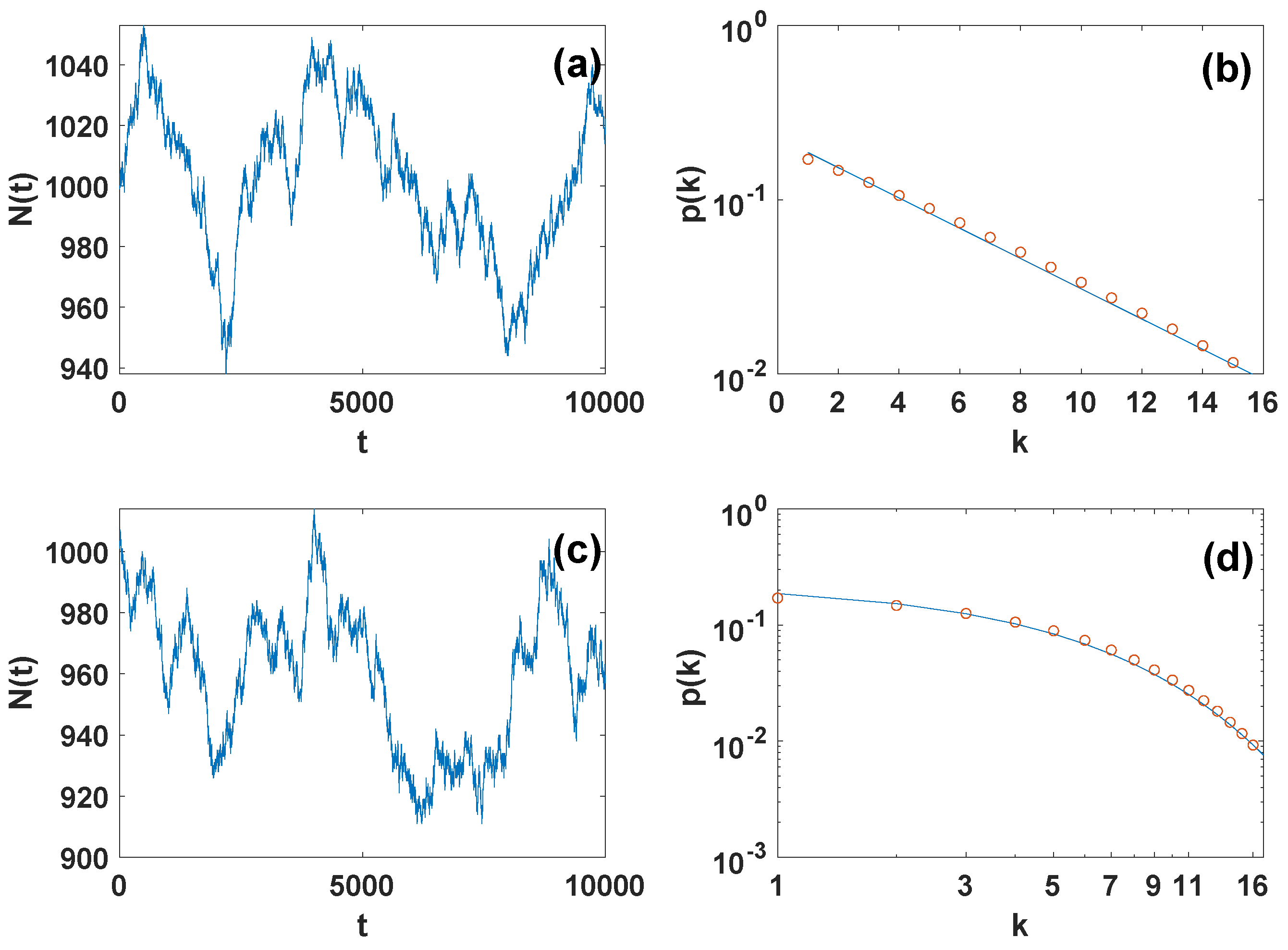
The Metropolis-Hastings algorithm can be used to sample the space of networks with variable number of nodes and given (stable) degree distribution (see Figure 2).
6.2. Monte Carlo Generation of Grand Canonical Network Ensemble with Given Latent Variable Distribution
A single instance of the grand canonical model with given latent variable distribution can be obtained by performing the following algorithm:
- 1
- Draw the network size N from the distribution;
- 2
- Draw the latent variable of each node i independently from the latent variable distribution .
- 3
- Draw each link of the network with probability .
7. Bayesian Estimation of the Network Parameters Given Partial Knowledge of the Network
In this section we will use the grand canonical network ensembles for calculating the posterior distribution of the network parameters given partial information of a network . In particular let us assume that we only know the subgraph induced by a set of nodes of nodes and of adjacency matrix and we do not have access to the full network G with adjacency matrix . Without loss of generality let us label the nodes of the network in such a way that the labels i with indicate the nodes in (denote as sampled nodes) and the labels i with indicate the nodes in (denoted also as unsampled or unknown nodes). We indicate with the degree sequence of the sampled network . Our goal is to make a Bayesian estimation of the network size N and the true network parameters given the observed subgraph . These a posteriori estimates of the true parameters of the network can then be used to reconstruct the unknown part of the network G.
7.1. Inferring the True Parameters with the Grand Canonical Ensemble with Given Degree Distribution
In this paragraph we will use the grand canonical ensemble with given degree distribution to find the posterior probability distribution of the network parameters. For convenience we will indicate with the true degree of the sampled nodes and we will indicate the true degree of the remaining unsampled nodes . To this end, using the Bayes rule we get the following expression for the posterior distribution of the network parameters given the observed subgraph
where
with given by
Here indicates the entropy of the network fo size N with degree sequence whose expression is given by the Bender-Canfield formula [3,21,22,47] (Equation (7)) which reads in this case
Moreover indicates the logarithm of the number of networks of N nodes having (with adjacency matrix and degree sequence ) as induced subgraph between the sampled nodes.
Moreover in Equation (31) indicates the evidence of the data given by
Calculating the entropy using statistical mechanics methods including the use of a functional order parameter (see Appendix A), we derive the following expression:
where M indicates the number of links between the sampled nodes and the unsampled nodes and Q indicates the sum over all the degrees of the unsampled nodes, i.e.,
where M and Q need to satisfy the constraint enforcing that the total number of true links is given by . Therefore, indicating with , we must impose
The expression obtained for the entropy implies that the asymptotic expression for the number of networks with N nodes, degree sequence having as a subgraph is given by (see Appendix A for the derivation)
This expression admits a simple combinatorial interpretation. In fact the networks with degree sequence having as subgraph can be constructed by adding (unsampled) links to the graph . The unsampled part of the network can be constructed by assigning to each node i with a number of stubs given by and to each node i with a number of stubs given by . The unsampled networks can then be obtained by matching the stubs pairwise with the constrains that the stubs of the first nodes can be only matched with the stubs of the unsampled nodes . Therefore the reconstructed part of the network is formed by a bipartite network between the sampled and the unsampled nodes with a number of links given by M and a simple network among the unsampled nodes with number of links given by . The number of matchings of the M links of the bipartite network is given by the number of matching of the stubs of the simple network among unsampled nodes is . In order to get the number of distinct networks G with degree sequence having as subgraph we need to divide by the number of permutations of the stubs belonging to the same nodes and we need to multiply by Q choose M indicating the number of ways in which we can choose the M stubs of the unsampled nodes to be matched with the stubs of the sampled nodes.
Given the expression for provided by Equation (36), we can deduce the explicit expression for :
It follows that the describe Bayesian inference assigns a probability to the model parameters a probability
with given by Equation (40). From this expression, imposing with a delta function that , expressing the delta in integral form and using the saddle point to evaluate the integral, we can calculate the marginal probability that a sampled node i with has true degree given M and Q, i.e.,
where is related to M by
In Figure 3 we show the difference between an exponential prior distribution on the degree of the nodes and the posterior marginal probability of the true degree of the sampled nodes plotted for different values of the sampled degree of the same node. Finally, we can calculate the a posteriori probability that the real networks has N nodes, conditioned to M and to the sampled subrgraph . To this end we sum Equation (41) over all the possible values of the degrees and such that Equation (37) are satisfied. Therefore, by inserting Equation (40) into Equation (41), enforcing Equation (37) with Kronecker deltas and integrating over all the possible values of and we get
where
where . By expressing the Kronecker deltas in an integral form according to the expression
performing a Wick rotation and evaluating the integrals at the saddle point, we can express and as
with and fixed by the saddle point equations
In Figure 4 we display the marginal a posteriori distribution as function of M demonstrating that the sampled network can modify significantly the prior assumptions on the total number of nodes in the network.
7.2. Inferring the True Parameters with the Grand Canonical Ensemble with Given Latent Variable Distribution
In this section we treat the problem of Bayesian estimation of the parameters of the true network G given the sampled network using the grand canonical model with given latent variable distribution. Let us indicate with the latent variables of the sampled nodes and with the latent variables of the unsampled nodes . Using Bayes rule we have
where is independent of , i.e., and where
with given by Equation (15) and with indicating the adjacency matrix of the sampled subgraph . In Equation (49) indicates the evidence of the data given by
Since, as we have observed previously, is independent of the Bayesian estimation of the parameters reduces simply to the prior in this case. Therefore we focus here only on the Bayesian estimate of the latent variables , i.e., we consider
with having the same definition as above and
Using the explicit expression of given by Equation (15), we can express the likelihood of the sampled network as
where is the number of links of the sampled network . In the limit we can approximate this expression as
with this approximation we get that the posterior probability is given by
Calculating the marginal posterior probability of a single latent variable conditional of we get
In Figure 3 we show the difference between an exponential prior distribution on the latent variables of the nodes and the posterior marginal probability of the true latent variables of the sampled nodes plotted for different values of the sampled degree of the same node.
Stating from Equation (56) we can also calculate the posterior distribution of the true number of nodes . To this end we express the delta function in an integral form and we sum over all possible latent variables , obtaining
where is given by
In Figure 4 we display the marginal a posteriori distribution on the true number of nodes in the simplified assumption in which is regular and all degree are the same demonstrating that the sampled network can modify significantly the prior assumptions on the total number of nodes in the network.
8. Conclusions
In this paper we have proposed grand canonical network ensembles formed by networks of varying number of nodes. The grand canonical network ensembles we have introduced are both sparse and exchangeable, i.e., have a finite average degree and are invariant under permutation of the node labels. The grand canonical ensembles are hierarchical network models in which first the network size is selected, then the degree sequence (or the sequence of latent variables) and finally the network adjacency matrix is selected. The model circumvents the difficulties imposed by the Aldous-Hoover theorem that states that exchangeable infinite sparse network ensembles vanish, as the network is a mixture of finite networks, although the networks can have an arbitrarily large network size. Here we show how the grand-canonical ensembles can be used to perform a Bayesian estimation of the network parameters when only partial information about the network structures is known. This a posteriori estimation of the network parameters can then be used for network reconstruction.
The grand canonical framework for sparse exchangeable network ensembles is here described for the case simple networks but has the potential to be extended to generalized network structures including directed, bipartite networks, multiplex networks and simplicial complexes following the lines outlined in ref. [32].
In conclusion we hope that this work, proposing hierarchical grand canonical network ensembles able to treat networks of different size and relating network theory to statistical mechanics will stimulate further results of mathematicians, physicists, and computer scientists working in network science and related machine learning problems.
Funding
G.B. acknowledges support from the Royal Society IEC\NSFC\191147.
Informed Consent Statement
Not applicable.
Data Availability Statement
Not applicable.
Conflicts of Interest
The author declares no conflict of interest.
Appendix A. Derivation of (k,q|κ)
In this Appendix our goal is to derive the asymptotic expression of in the limit of large network size of the sampled network , and of the true network with .
Let us assume that the sampled subgraph G is the network between the sampled nodes and has adjacency matrix . The true network is instead formed by N nodes with adjacency matrix . We assume that has the block structure given by
where indicates the matrix between sampled nodes and the unsampled nodes and indicates tha adjacency matrix among the unsampled nodes. As we have mentioned in the main text is the logarithm of the number of networks (or adjacency matrices ) with degree sequence and admitting as a subgraph having sampled degree sequence . In statistical mechanics we also call the partition function of its corresponding statistical mechanics network model, and we indicate it by Z. In terms of the matrices and the partition function can be written as
Expressing the Kronecker deltas in the integral form and performing the sum over the elements of the matrices and we obtain
with
and with and . Let us now introduce the functional order parameters [22,49,50].
where is the fraction of sampled nodes with degree in the sampled network and total inferred degree k; is the fraction of unsampled nodes with degree q. Moreover we have indicated with and with . By enforcing the definition of the order parameters with a series of delta functions we obtain
After inserting these expressions into the partition function in the limit , indicating with the sum over the allowed degree range we obtain
with given by
where is given by
and where the functional measures are defined as
By putting
and performing a Wick rotation in and assuming real and much smaller than one, i.e., which is allowed in the sparse regime, we can linearize the logarithm and express as
with
The saddle point equations determining the value of the partition function can be obtained by performing the (functional) derivative of f with respect to the functional order parameters, obtaining
Let us first calculate the integrals
Using these expressions for the integral we can write the functional order parameters as
With this expression, using a similar procedure we can express as
Combing these equations with the last saddle point equation it is immediate to show that and are given by
with
Calculating the free energy at the saddle point, we get
which leads to the following asymptotic expression for
References
- Barabási, A.L. Network Science; Cambridge University Press: Cambridge, UK, 2016. [Google Scholar]
- Newman Mark, E. Networks: An Introduction; Oxford University Press: Cambridge, UK, 2010. [Google Scholar]
- Anand, K.; Bianconi, G. Entropy measures for networks: Toward an information theory of complex topologies. Phys. Rev. E 2009, 80, 045102. [Google Scholar] [CrossRef] [PubMed] [Green Version]
- Park, J.; Newman, M.E. Statistical mechanics of networks. Phys. Rev. E 2004, 70, 066117. [Google Scholar] [CrossRef] [PubMed] [Green Version]
- Bianconi, G. Information theory of spatial network ensembles. In Handbook on Entropy, Complexity and Spatial Dynamics; Edward Elgar Publishing: Cheltenham, UK, 2021. [Google Scholar]
- Cimini, G.; Squartini, T.; Saracco, F.; Garlaschelli, D.; Gabrielli, A.; Caldarelli, G. The statistical physics of real-world networks. Nat. Rev. Phys. 2019, 1, 58–71. [Google Scholar] [CrossRef] [Green Version]
- Krioukov, D.; Papadopoulos, F.; Kitsak, M.; Vahdat, A.; Boguná, M. Hyperbolic geometry of complex networks. Phys. Rev. E 2010, 82, 036106. [Google Scholar] [CrossRef] [PubMed] [Green Version]
- Orsini, C.; Dankulov, M.M.; Colomer-de Simón, P.; Jamakovic, A.; Mahadevan, P.; Vahdat, A.; Bassler, K.E.; Toroczkai, Z.; Boguná, M.; Caldarelli, G.; et al. Quantifying randomness in real networks. Nat. Commun. 2015, 6, 8627. [Google Scholar] [CrossRef]
- Peixoto, T.P. Entropy of stochastic blockmodel ensembles. Phys. Rev. E 2012, 85, 056122. [Google Scholar] [CrossRef] [Green Version]
- Radicchi, F.; Krioukov, D.; Hartle, H.; Bianconi, G. Classical information theory of networks. J. Phys. Complex. 2020, 1, 025001. [Google Scholar] [CrossRef]
- Pessoa, P.; Costa, F.X.; Caticha, A. Entropic dynamics on Gibbs statistical manifolds. Entropy 2021, 23, 494. [Google Scholar] [CrossRef]
- Kim, H.; Del Genio, C.I.; Bassler, K.E.; Toroczkai, Z. Constructing and sampling directed graphs with given degree sequences. New J. Phys. 2012, 14, 023012. [Google Scholar] [CrossRef] [Green Version]
- Del Genio, C.I.; Kim, H.; Toroczkai, Z.; Bassler, K.E. Efficient and exact sampling of simple graphs with given arbitrary degree sequence. PLoS ONE 2010, 5, e10012. [Google Scholar] [CrossRef] [Green Version]
- Coolen, A.C.; Annibale, A.; Roberts, E. Generating Random Networks and Graphs; Oxford University Press: Oxford, UK, 2017. [Google Scholar]
- Bassler, K.E.; Del Genio, C.I.; Erdős, P.L.; Miklós, I.; Toroczkai, Z. Exact sampling of graphs with prescribed degree correlations. New J. Phys. 2015, 17, 083052. [Google Scholar] [CrossRef]
- Barabási, A.L.; Albert, R. Emergence of scaling in random networks. Science 1999, 286, 509–512. [Google Scholar] [CrossRef] [PubMed] [Green Version]
- Dorogovtsev, S.N.; Dorogovtsev, S.N.; Mendes, J.F. Evolution of Networks: From Biological Nets to the Internet and WWW; Oxford University Press: Oxford, UK, 2003. [Google Scholar]
- Kharel, S.R.; Mezei, T.R.; Chung, S.; Erdős, P.L.; Toroczkai, Z. Degree-preserving network growth. Nat. Phys. 2021, 18, 100–106. [Google Scholar] [CrossRef]
- Jaynes, E.T. Information theory and statistical mechanics. Phys. Rev. 1957, 106, 620. [Google Scholar] [CrossRef]
- Huang, K. Introduction to Statistical Physics; Chapman and Hall: London, UK; CRC: Boca Raton, FL, USA, 2009. [Google Scholar]
- Anand, K.; Bianconi, G. Gibbs entropy of network ensembles by cavity methods. Phys. Rev. E 2010, 82, 011116. [Google Scholar] [CrossRef] [PubMed] [Green Version]
- Bianconi, G.; Coolen, A.C.; Vicente, C.J.P. Entropies of complex networks with hierarchically constrained topologies. Phys. Rev. E 2008, 78, 016114. [Google Scholar] [CrossRef] [Green Version]
- Caldarelli, G.; Capocci, A.; De Los Rios, P.; Munoz, M.A. Scale-free networks from varying vertex intrinsic fitness. Phys. Rev. Lett. 2002, 89, 258702. [Google Scholar] [CrossRef] [Green Version]
- Bianconi, G.; Pin, P.; Marsili, M. Assessing the relevance of node features for network structure. Proc. Natl. Acad. Sci. USA 2009, 106, 11433–11438. [Google Scholar] [CrossRef] [Green Version]
- Airoldi, E.M.; Blei, D.; Fienberg, S.; Xing, E. Mixed membership stochastic blockmodels. Adv. Neural Inf. Process. Syst. 2008, 21, 1981–2014. [Google Scholar]
- Ghavasieh, A.; Nicolini, C.; De Domenico, M. Statistical physics of complex information dynamics. Phys. Rev. E 2020, 102, 052304. [Google Scholar] [CrossRef]
- Bevilacqua, B.; Zhou, Y.; Ribeiro, B. Size-invariant graph representations for graph classification extrapolations. In Proceedings of the International Conference on Machine Learning, PMLR, London, UK, 8–11 November 2021; pp. 837–851. [Google Scholar]
- Cotta, L.; Morris, C.; Ribeiro, B. Reconstruction for powerful graph representations. Adv. Neural Inf. Process. Syst. 2021, 34. [Google Scholar] [CrossRef]
- De Finetti, B. Funzione Caratteristica Di un Fenomeno Aleatorio; Accademia Nazionale Lincei: Rome, Italy, 1931; Volume 4. [Google Scholar]
- Lovász, L. Large Networks and Graph Limits; American Mathematical Society: Providence, RI, USA, 2012; Volume 60. [Google Scholar]
- Chung, F.; Lu, L. The average distances in random graphs with given expected degrees. Proc. Natl. Acad. Sci. USA 2002, 99, 15879–15882. [Google Scholar] [CrossRef] [PubMed] [Green Version]
- Bianconi, G. Statistical physics of exchangeable sparse simple networks, multiplex networks, and simplicial complexes. Phys. Rev. E 2022, 105, 034310. [Google Scholar] [CrossRef] [PubMed]
- Caron, F.; Fox, E.B. Sparse graphs using exchangeable random measures. J. R. Stat. Soc. Ser. Stat. Methodol. 2017, 79, 1295. [Google Scholar] [CrossRef] [PubMed] [Green Version]
- Borgs, C.; Chayes, J.T.; Cohn, H.; Holden, N. Sparse exchangeable graphs and their limits via graphon processes. arXiv 2016, arXiv:1601.07134. [Google Scholar]
- Veitch, V.; Roy, D.M. The class of random graphs arising from exchangeable random measures. arXiv 2015, arXiv:1512.03099. [Google Scholar]
- Veitch, V.; Roy, D.M. Sampling and estimation for (sparse) exchangeable graphs. Ann. Stat. 2019, 47, 3274–3299. [Google Scholar] [CrossRef] [Green Version]
- Borgs, C.; Chayes, J.T.; Smith, A. Private graphon estimation for sparse graphs. arXiv 2015, arXiv:1506.06162. [Google Scholar]
- Borgs, C.; Chayes, J.; Smith, A.; Zadik, I. Revealing network structure, confidentially: Improved rates for node-private graphon estimation. In Proceedings of the 2018 IEEE 59th Annual Symposium on Foundations of Computer Science (FOCS), Paris, France, 7–9 October 2018; pp. 533–543. [Google Scholar]
- Bianconi, G. Multilayer Networks: Structure and Function; Oxford University Press: Oxford, UK, 2018. [Google Scholar]
- Bianconi, G. Higher-Order Networks: An Introduction to Simplicial Complexes; Cambridge University Press: Cambridge, UK, 2021. [Google Scholar]
- Aldous, D.J. Representations for partially exchangeable arrays of random variables. J. Multivar. Anal. 1981, 11, 581–598. [Google Scholar] [CrossRef] [Green Version]
- Hoover, D.N. Relations on Probability Spaces and Arrays of Random Variables; Institute for Advanced Study: Princeton, NJ, USA, 1979; Volume 2, p. 275. [Google Scholar]
- Paton, J.; Hartle, H.; Stepanyants, J.; van der Hoorn, P.; Krioukov, D. Entropy of labeled versus unlabeled networks. arXiv 2022, arXiv:2204.08508. [Google Scholar]
- Peixoto, T.P. Hierarchical block structures and high-resolution model selection in large networks. Phys. Review X 2014, 4, 011047. [Google Scholar] [CrossRef] [Green Version]
- Gabrielli, A.; Mastrandrea, R.; Caldarelli, G.; Cimini, G. Grand canonical ensemble of weighted networks. Phys. Rev. E 2019, 99, 030301. [Google Scholar] [CrossRef] [PubMed] [Green Version]
- Straka, M.J.; Caldarelli, G.; Saracco, F. Grand canonical validation of the bipartite international trade network. Phys. Rev. E 2017, 96, 022306. [Google Scholar] [CrossRef] [PubMed] [Green Version]
- Bender, E.A.; Canfield, E.R. The asymptotic number of labeled graphs with given degree sequences. J. Comb. Theory Ser. A 1978, 24, 296–307. [Google Scholar] [CrossRef] [Green Version]
- Bianconi, G. Entropy of network ensembles. Phys. Rev. E 2009, 79, 036114. [Google Scholar] [CrossRef] [Green Version]
- Courtney, O.T.; Bianconi, G. Generalized network structures: The configuration model and the canonical ensemble of simplicial complexes. Phys. Rev. E 2016, 93, 062311. [Google Scholar] [CrossRef] [Green Version]
- Monasson, R.; Zecchina, R. Statistical mechanics of the random K-satisfiability model. Phys. Rev. E 1997, 56, 1357. [Google Scholar] [CrossRef] [Green Version]
Figure 1.
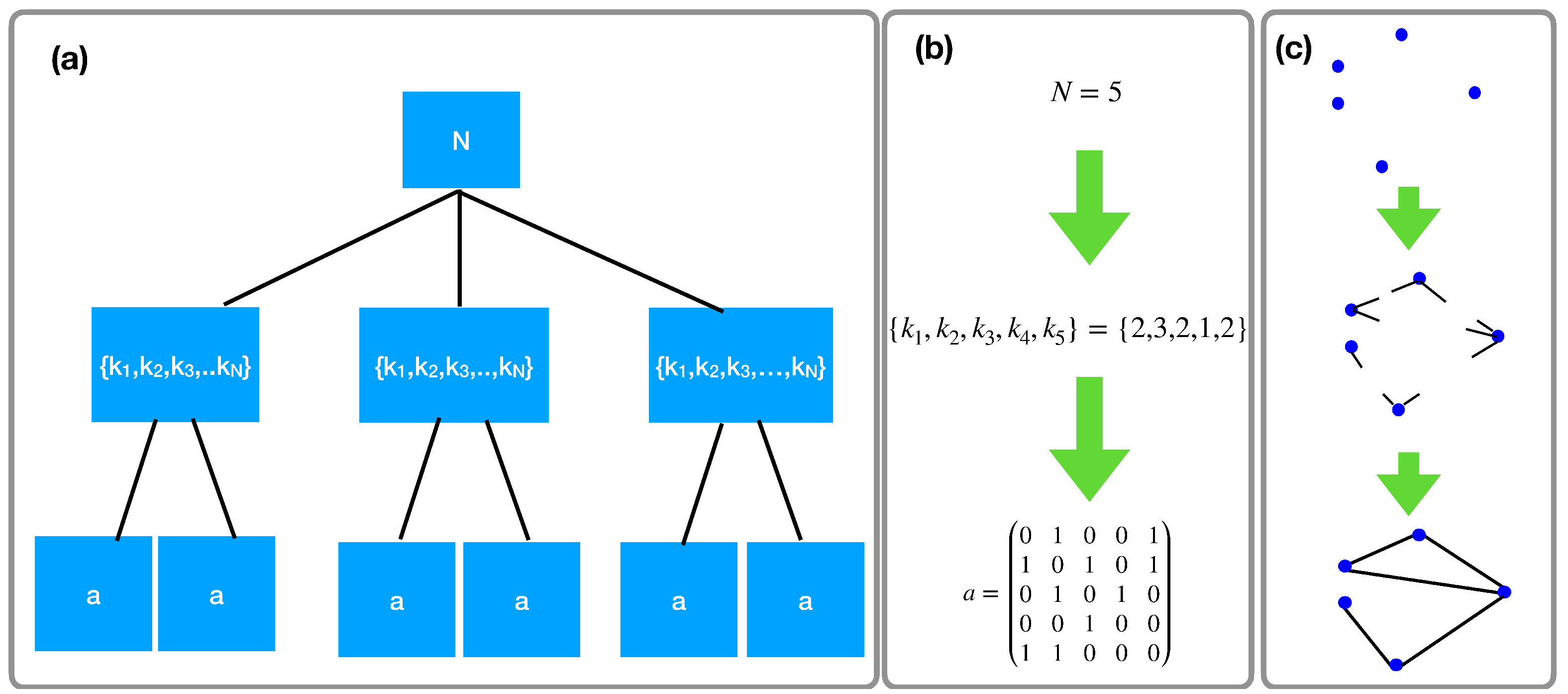
Schematic representation of the hierarchical grand canonical ensemble of exchangeable sparse simple networks. The proposed ensemble is a hierarchical model of networks in which first the total number of nodes N is drawn from a distribution, then a given degree sequence is drawn from the distribution among all the degree sequence with the total number of nodes N; finally a network G with adjacency matrix drawn from the distribution among all the networks with a given total number of nodes N and degree sequence . Panel (a) describes the hierarchical nature of the model, panel (b) provide an example of subsequent draw of the total number of nodes, the degree sequence and the adjacency matrix of the network, panel (c) is a visualization of the construction of a network according to the proposed model.
Figure 1.
Schematic representation of the hierarchical grand canonical ensemble of exchangeable sparse simple networks. The proposed ensemble is a hierarchical model of networks in which first the total number of nodes N is drawn from a distribution, then a given degree sequence is drawn from the distribution among all the degree sequence with the total number of nodes N; finally a network G with adjacency matrix drawn from the distribution among all the networks with a given total number of nodes N and degree sequence . Panel (a) describes the hierarchical nature of the model, panel (b) provide an example of subsequent draw of the total number of nodes, the degree sequence and the adjacency matrix of the network, panel (c) is a visualization of the construction of a network according to the proposed model.

Figure 2.
Results of the Metropolis-Hastings algorithm for generating grand canonical ensembles with given degree distribution. The number of nodes as a function of time t in the Metropolis-Hastings simulation of an exponential networks (panel (a)) and networks with more general degree distribution (panel (c)) are shown together with the average degree distribution of the networks that is stable as the number of networks varies (symbols of panel (b) and (d)). The solid lines in panel (b) and panel (d) indicate the target degree distributions with (for panel (b)) and with (for panel (d)). The prior on the number of nodes is taken to be exponential with with and .

Figure 3.
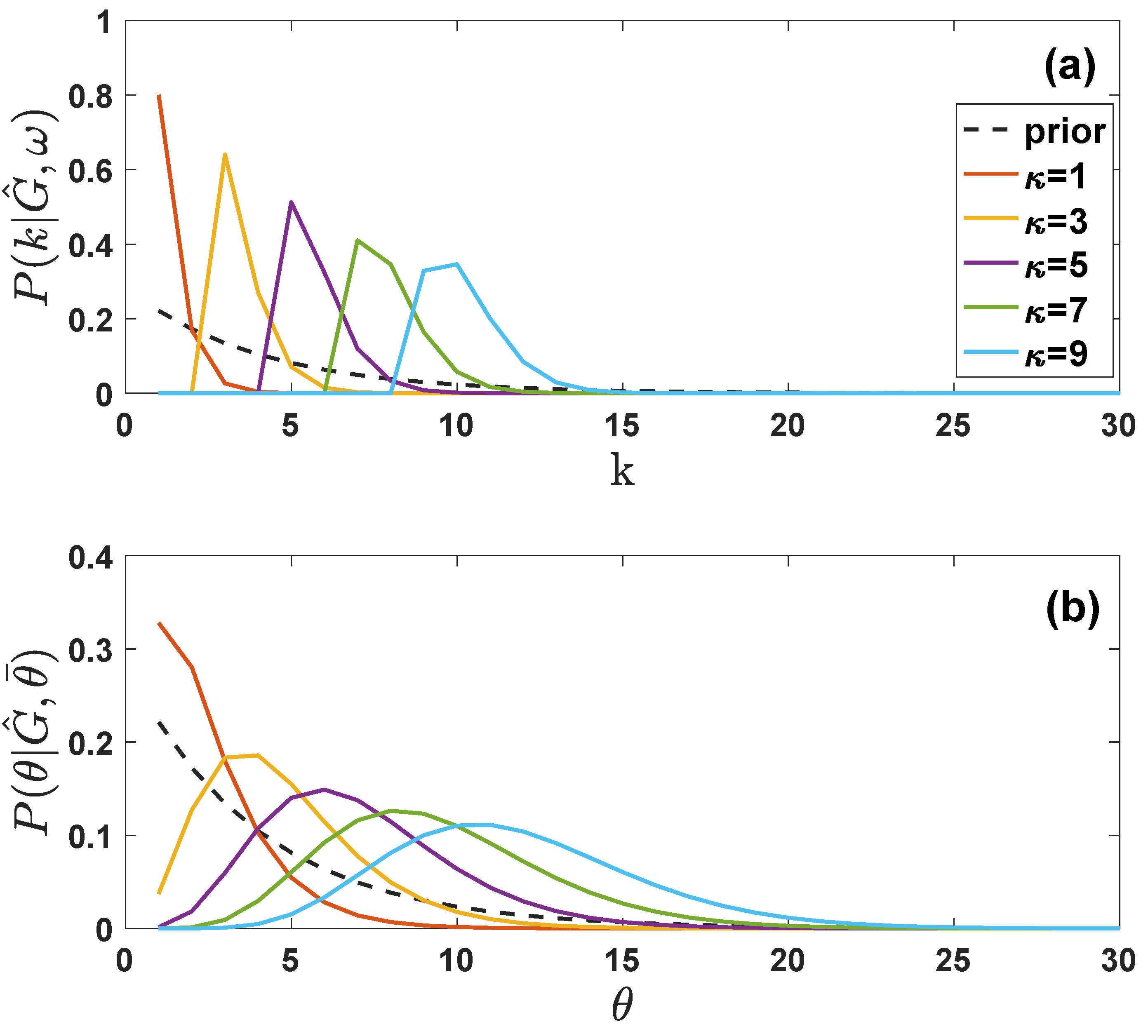
Marginal posterior probability for the true degree and of the true latent variable of a sampled node. The posterior probability (panel (a)) of the true degree of a sampled nodes depends on the degree of the nodes in the sampled network and is non-zero only for . The posterior probability of the latent variable of a sampled node (panel (b)) can be non-zero on the entire range of values allowed by the prior. Here we have plotted and for different values of and we have chosen and . The dashed lines indicate the exponential prior on the degrees (panel (a)) and on the latent variables (panel (b)).
Figure 3.
Marginal posterior probability for the true degree and of the true latent variable of a sampled node. The posterior probability (panel (a)) of the true degree of a sampled nodes depends on the degree of the nodes in the sampled network and is non-zero only for . The posterior probability of the latent variable of a sampled node (panel (b)) can be non-zero on the entire range of values allowed by the prior. Here we have plotted and for different values of and we have chosen and . The dashed lines indicate the exponential prior on the degrees (panel (a)) and on the latent variables (panel (b)).

Figure 4.
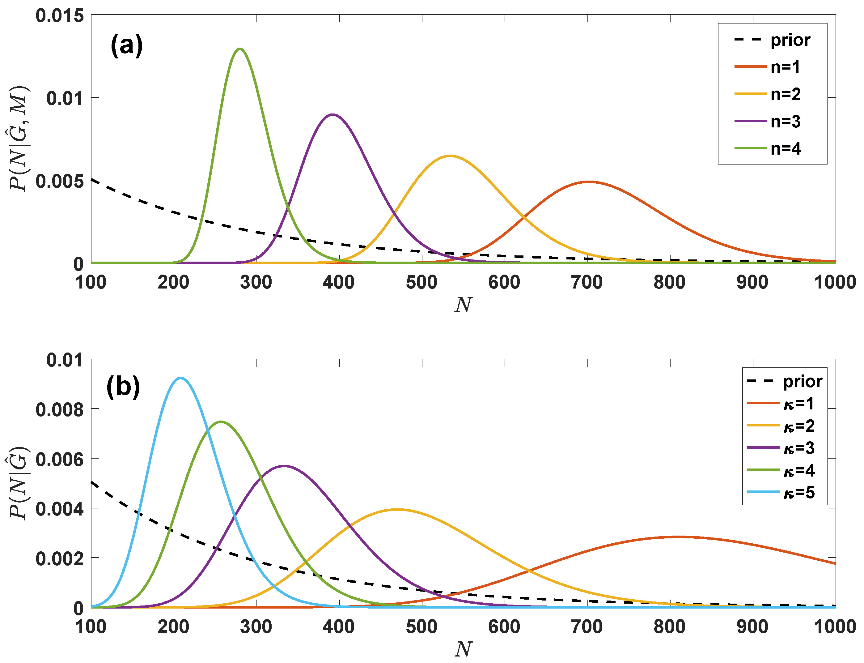
Marginal posterior probability for the true number of nodes in the grand canonical ensemble with given degree distribution and in the grand canonical ensemble with given latent variable distribution. The posterior probability in panel (a) of the true number of nodes depends on the total number M of true but not observed links of the sampled nodes and on the total number of sampled links ; the posterior probability in panel (b) depends instead only on the degree of the nodes in the sampled network . We took and the priors given by , , with , and . In panel (a) we have plotted for different values of with and ; in panel (b) we have plotted assuming that is regular with all sampled nodes having sampled degree . The dashed lines indicate the exponential prior on the number of nodes.
Figure 4.
Marginal posterior probability for the true number of nodes in the grand canonical ensemble with given degree distribution and in the grand canonical ensemble with given latent variable distribution. The posterior probability in panel (a) of the true number of nodes depends on the total number M of true but not observed links of the sampled nodes and on the total number of sampled links ; the posterior probability in panel (b) depends instead only on the degree of the nodes in the sampled network . We took and the priors given by , , with , and . In panel (a) we have plotted for different values of with and ; in panel (b) we have plotted assuming that is regular with all sampled nodes having sampled degree . The dashed lines indicate the exponential prior on the number of nodes.

Publisher’s Note: MDPI stays neutral with regard to jurisdictional claims in published maps and institutional affiliations. |
© 2022 by the author. Licensee MDPI, Basel, Switzerland. This article is an open access article distributed under the terms and conditions of the Creative Commons Attribution (CC BY) license (https://creativecommons.org/licenses/by/4.0/).
Share and Cite
MDPI and ACS Style
Bianconi, G. Grand Canonical Ensembles of Sparse Networks and Bayesian Inference. Entropy 2022, 24, 633. https://doi.org/10.3390/e24050633
AMA Style
Bianconi G. Grand Canonical Ensembles of Sparse Networks and Bayesian Inference. Entropy. 2022; 24(5):633. https://doi.org/10.3390/e24050633
Chicago/Turabian StyleBianconi, Ginestra. 2022. "Grand Canonical Ensembles of Sparse Networks and Bayesian Inference" Entropy 24, no. 5: 633. https://doi.org/10.3390/e24050633
Note that from the first issue of 2016, this journal uses article numbers instead of page numbers. See further details here.