
OxDNA to Study Species Interactions

 ,
,  , , , and
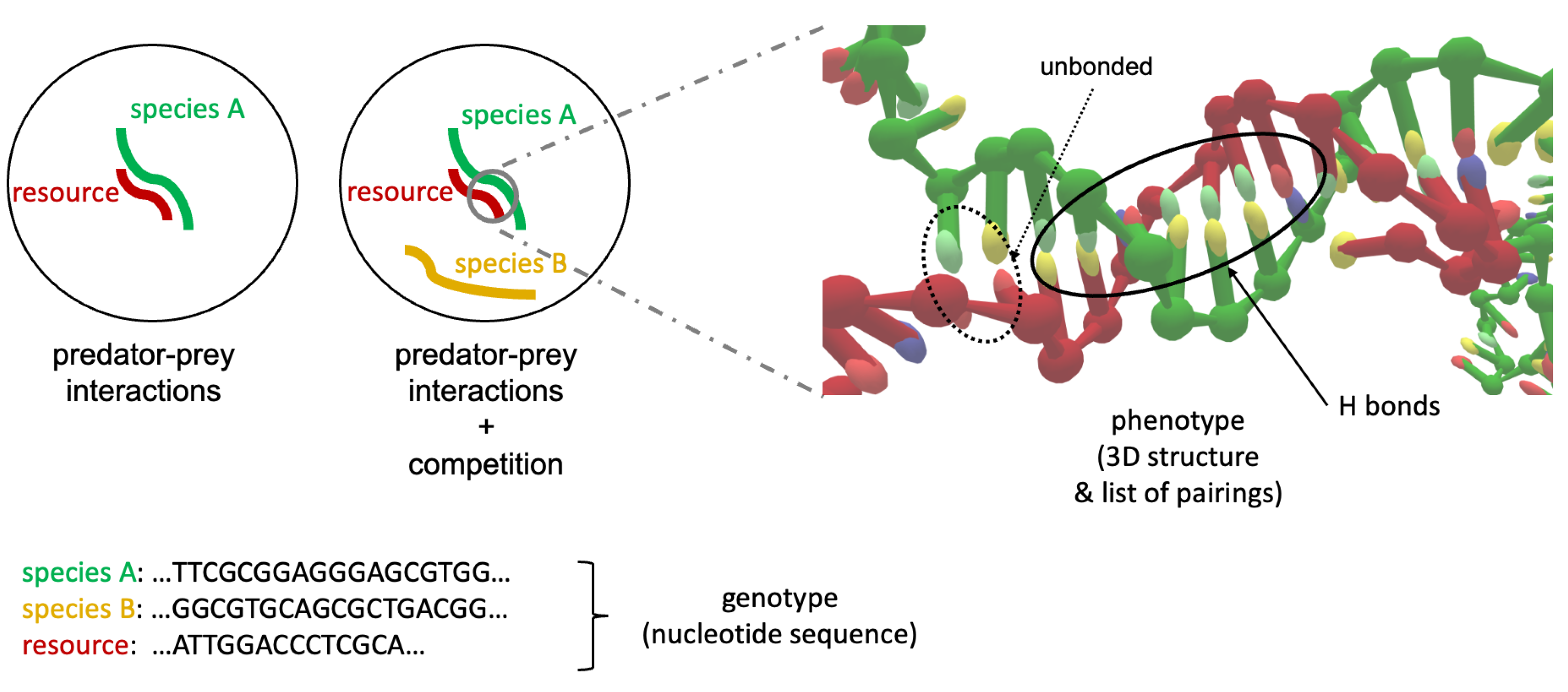
Abstract
:1. Introduction
2. Materials and Methods
2.1. Simulations
- system initialization;
- minimization steps, ≈75 ps (where each strand reaches its own minimum energy configuration);
- relax phase: MD steps (≈1.5155 s) where the system is subjected to external forces which trigger the interactions and softly enhance the formation of hydrogen bonds (HBs). In particular, strands are usually enforced to form their best attachment (see next subsection for an extended discussion concerning how we evaluate the strength of a bond between DNA strands) and are weakly attracted towards the center of the box, to prevent excessive diffusion. Temperature and volume are kept constant;
- MD simulation: MD steps where the system is not subjected to external forces anymore and freely evolves in a box at a constant volume and temperature.
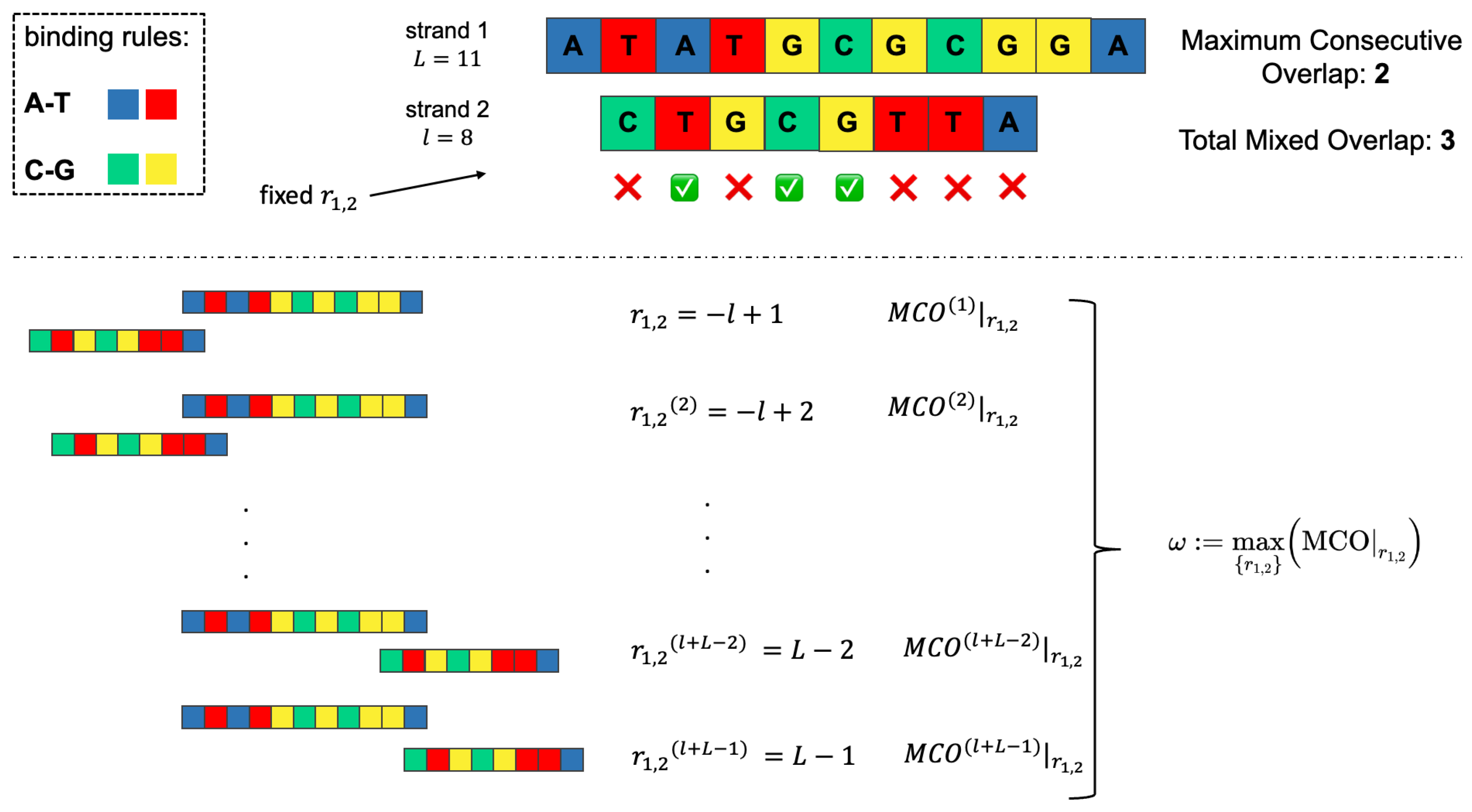
2.2. Overlap Metrics
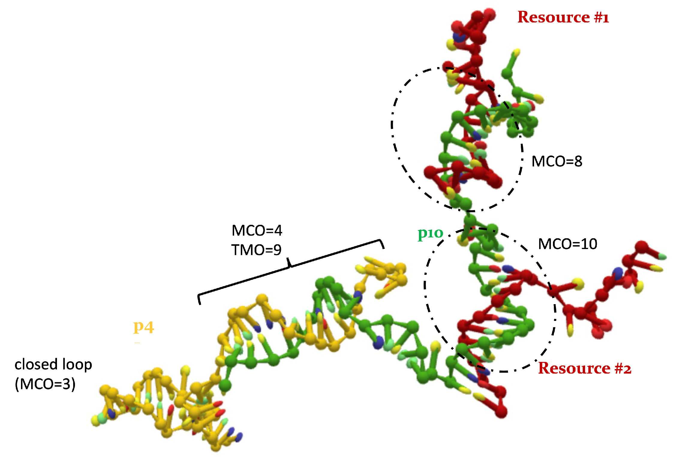
- the Maximum Consecutive Overlap (MCO), i.e., the largest number of consecutive matching bases (2, in the example);
- the Total Mixed Overlap (TMO), i.e., the total number of paired nucleotides in that position (3, in the example). It holds that: TMO≥ MCO, .
2.3. Experimental Methods
2.3.1. Sample Preparation
2.3.2. Polyacrylamide Gel Electrophoresis
3. Results
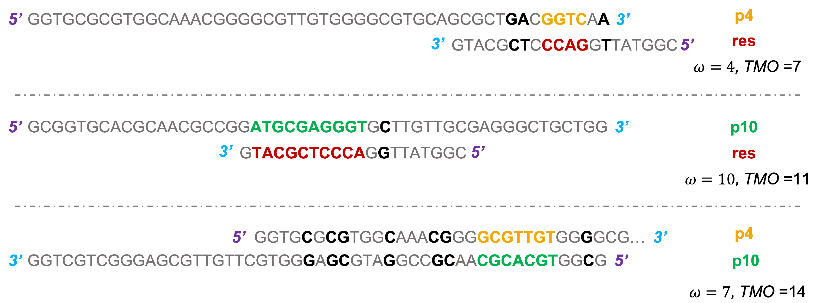
- a p4 and a resource;
- a p10 and a resource;
- two p4 strands;
- two p10 strands;
- a p4 and a p10;
- a p4, a p10 and a resource.
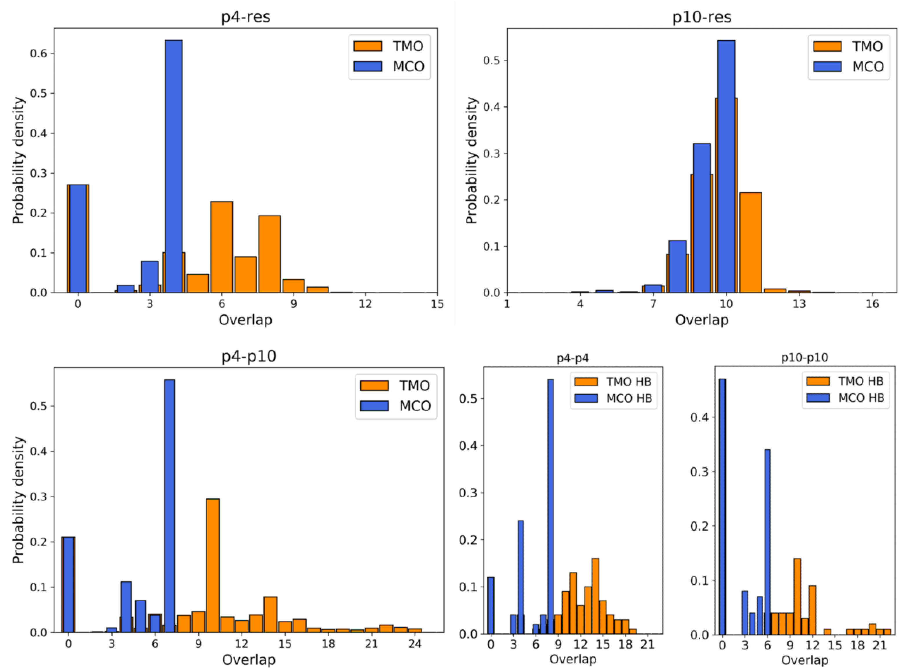
3.1. Simulation Results
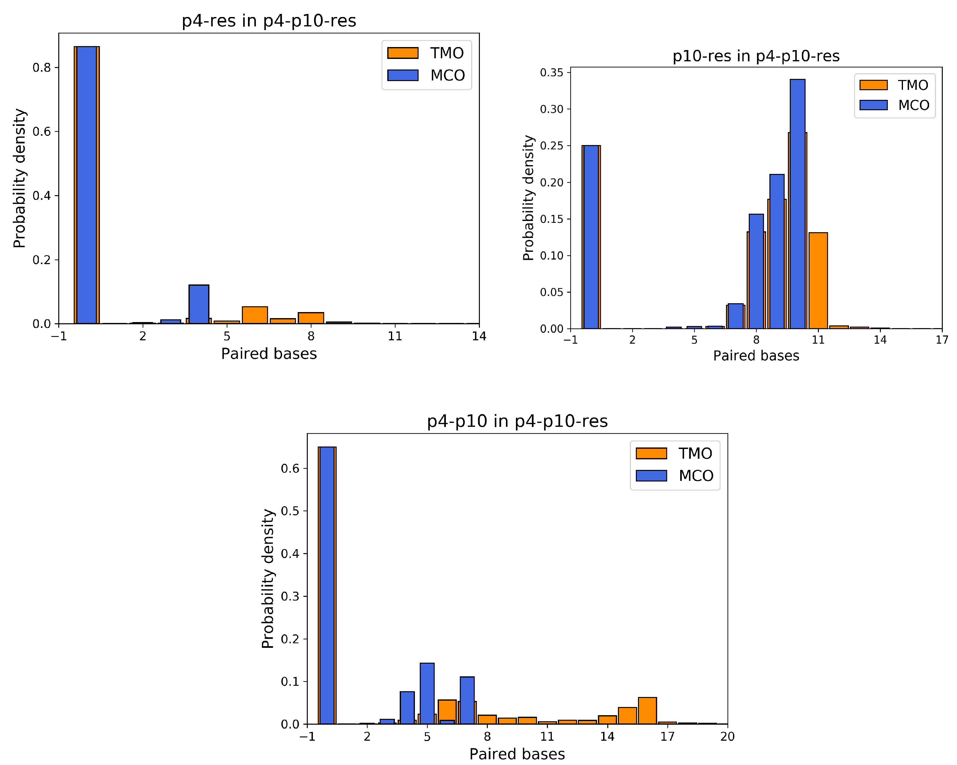
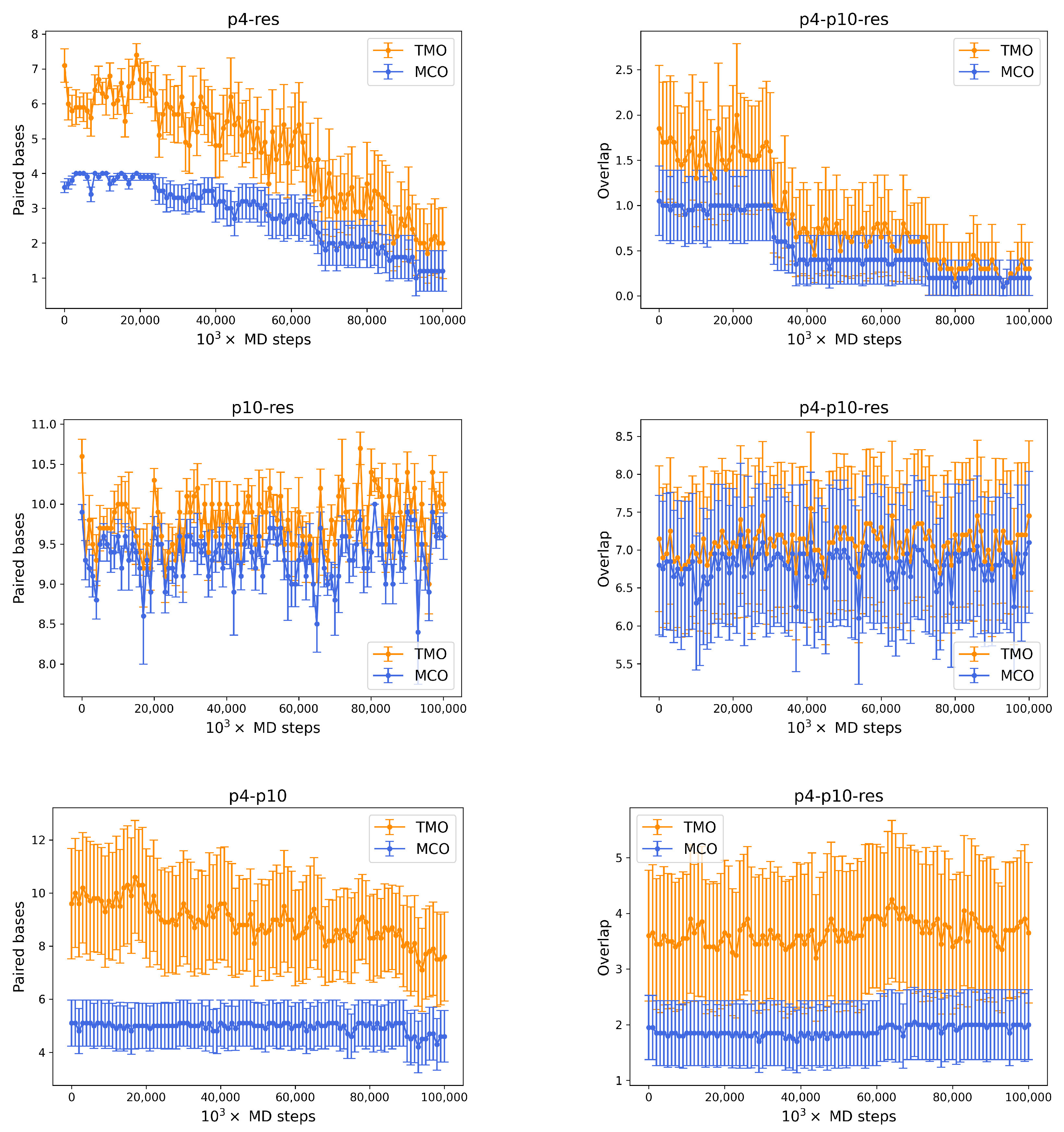
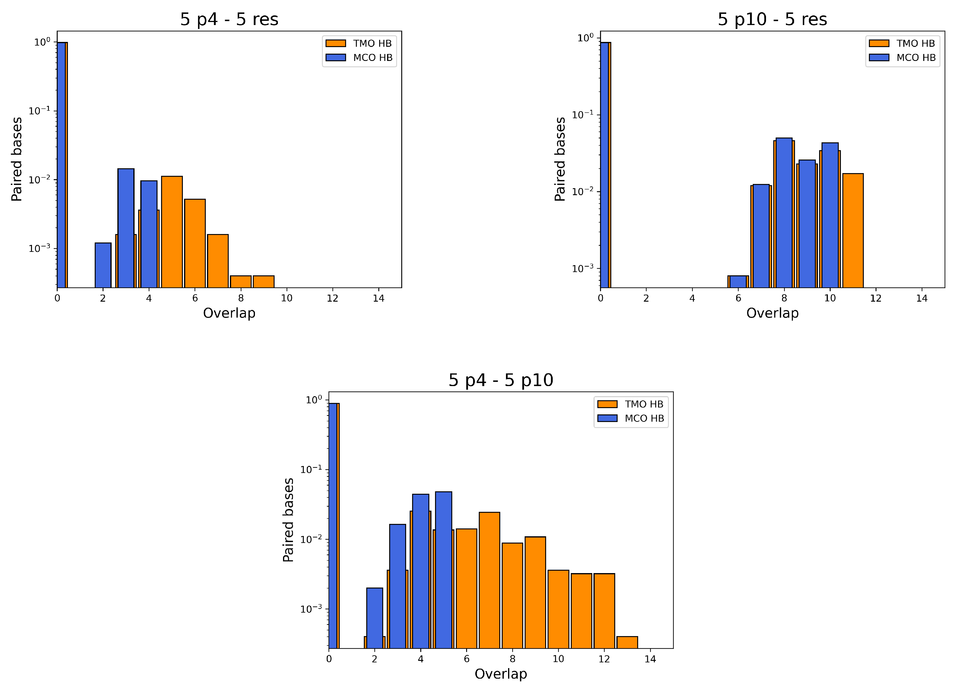
- between p4 and the resource is 4. During simulations, the actual MCO is exactly equal to for more than 60% of the timesteps. The top left panel of Figure 4 also shows that the two strands are not bonded for roughly 25% of the time, while they can also bind and form additional HBs (with a TMO of even 8 or 9). The interaction between this predator and the target strand can be thus described as quite weak, since is small and even the TMO is not very large. We underline that four consecutive paired bases represent the minimum threshold for having an effective attachment between two strands: with a smaller number of bases, the two strands are not going to even bend and their HBs can be easily broken.
- The actual MCO between p10 and the resource is equal to for more than 50% of the timesteps (see top right panel of Figure 4), and it is equal to for more than 30% of the cases. Here, it is also evident that the TMO does not play a key role, compared to the MCO, since they have very similar distribution, with TMO usually being larger at most by 1 or 2. MD simulations with oxDNA suggest, thus, that the MCO onset, maybe with one additional HB formed, is the preferred way for these strands to interact. This result can be interpreted as a much stronger binding than the p4-res case.
- The interaction between p4 and p10, without the resource, in more than 50% of the cases occurring via the formation of an MCO (see Figure 4, bottom left panel). Interestingly, in about 30% of the cases, we record a TMO = 10, with a distribution of the other TMO values mainly uniformly distributed between 4 and 9 and 11 and 16 HBs. The TMO distribution features a very long right tail, indicating that rarely a huge number of nucleotides can bind between the two oligomers. In the absence of the target strand, computer simulations suggest that these two predators can bind, and this might undoubtedly alter the interaction between each of them and the resource in an environment with these three species, as we will show later in this study.
- If two p4 strands interact, their is moderately high (8), and it roughly occurs 50% of the time (see Figure 4, bottom row, middle). In about 25% of the cases, the two strands have an MCO = 4, while in about 10% they are not bonded. Interestingly, they can form very large TMOs: the TMO distribution is bell-shaped, between 6 and 19. This means that two individuals of this species may mutually attract in a significant way, possibly with a high number of HBs, in different positions along the strands.
- Two p10 strands have , which during the simulation occurs with a frequency slightly larger than 30%. It has to be considered that this is possibly the prevalent form of binding between these two ssDNAs, since with almost 50% probability they do not share HBs. Such an interaction between two p10 strands can be classified as weaker than the p4-p4 one.
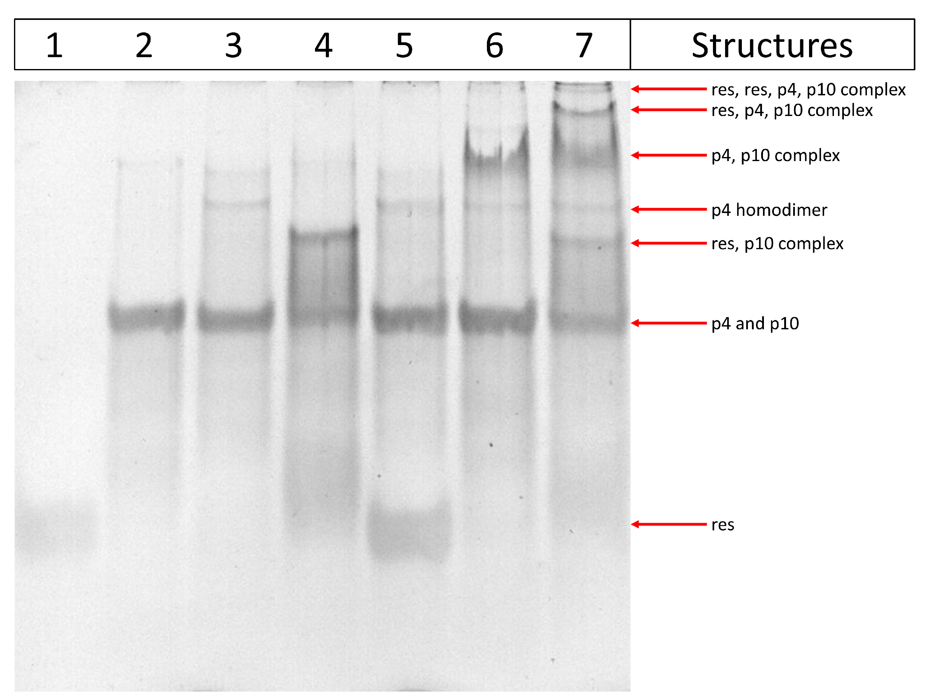
3.2. Experimental Results with Gels
Polyacrylamide Gel Electrophoresis
4. Discussion
5. Conclusions
Author Contributions
Funding
Institutional Review Board Statement
Informed Consent Statement
Data Availability Statement
Acknowledgments
Conflicts of Interest
Appendix A. Additional Simulation Results
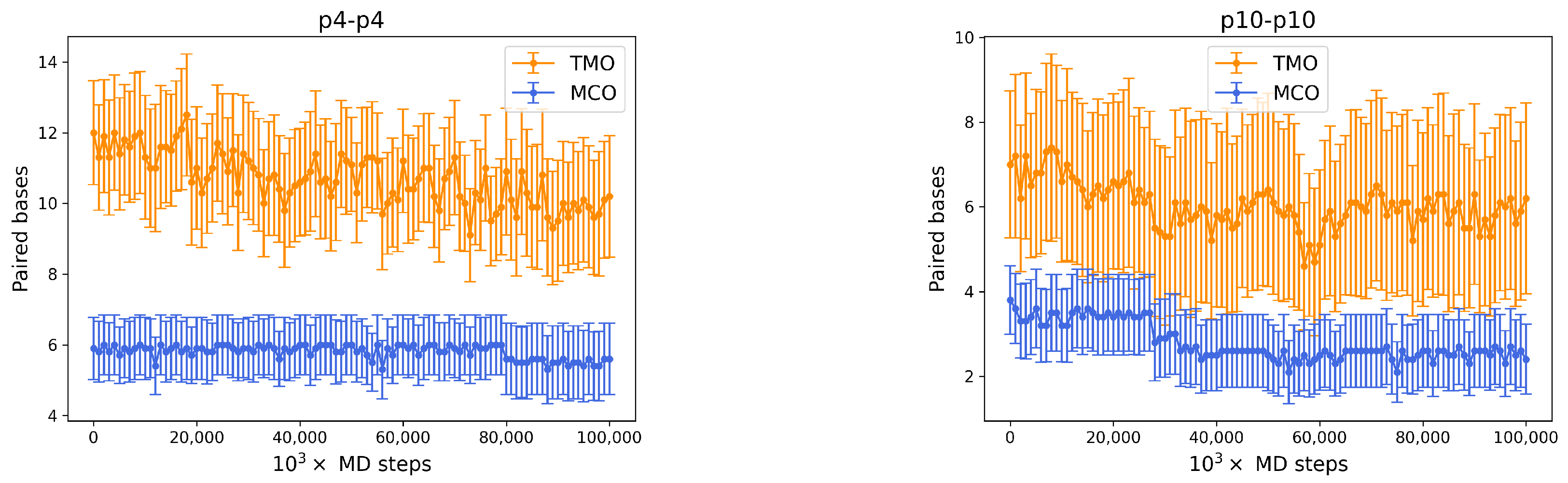
Appendix A.1. p4-p4 and p10-p10 HB Stability in Time

Appendix A.2. 4 Body Structures

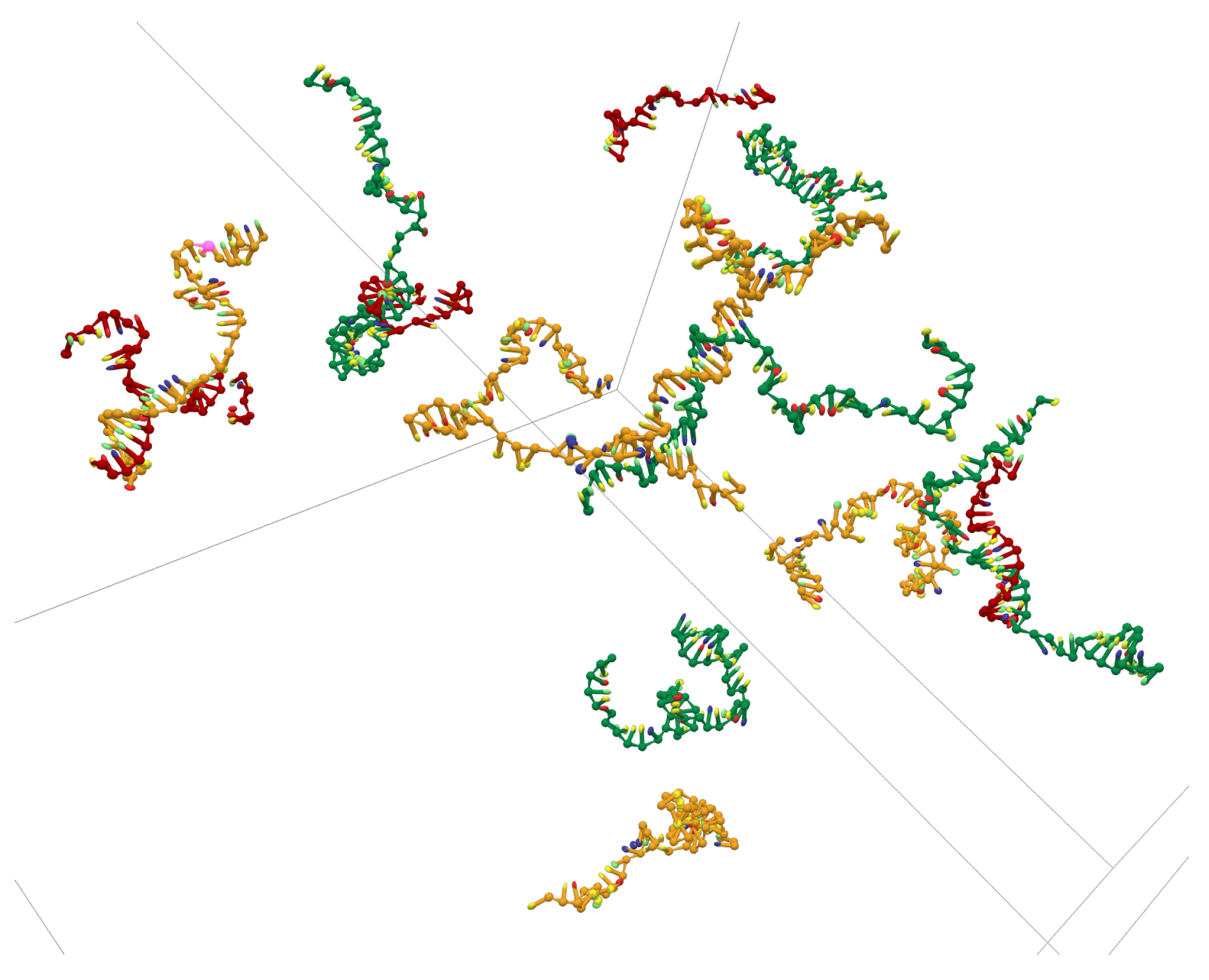
Appendix A.3. Simulation Cell with 15 ssDNAs


References
- Bascompte, J.; Jordano, P. Plant-animal mutualistic networks: The architecture of biodiversity. Annu. Rev. Ecol. Evol. Syst. 2007, 38, 567–593. [Google Scholar] [CrossRef] [Green Version]
- Hagen, M.; Kissling, W.D.; Rasmussen, C.; De Aguiar, M.A.; Brown, L.E.; Carstensen, D.W.; Alves-Dos-Santos, I.; Dupont, Y.L.; Edwards, F.K.; Genini, J.; et al. Biodiversity, species interactions and ecological networks in a fragmented world. Adv. Ecol. Res. 2012, 46, 89–210. [Google Scholar]
- Suweis, S.; Simini, F.; Banavar, J.R.; Maritan, A. Emergence of structural and dynamical properties of ecological mutualistic networks. Nature 2013, 500, 449–452. [Google Scholar] [CrossRef] [Green Version]
- Tu, C.; Suweis, S.; Grilli, J.; Formentin, M.; Maritan, A. Reconciling cooperation, biodiversity and stability in complex ecological communities. Sci. Rep. 2019, 9, 5580. [Google Scholar] [CrossRef] [PubMed] [Green Version]
- Ratzke, C.; Barrere, J.; Gore, J. Strength of species interactions determines biodiversity and stability in microbial communities. Nat. Ecol. Evol. 2020, 4, 376–383. [Google Scholar] [CrossRef] [PubMed]
- Chesson, P. MacArthur’s consumer-resource model. Theor. Popul. Biol. 1990, 37, 26–38. [Google Scholar] [CrossRef]
- Allesina, S.; Tang, S. Stability criteria for complex ecosystems. Nature 2012, 483, 205–208. [Google Scholar] [CrossRef] [Green Version]
- Suweis, S.; Grilli, J.; Maritan, A. Disentangling the effect of hybrid interactions and of the constant effort hypothesis on ecological community stability. Oikos 2014, 123, 525–532. [Google Scholar] [CrossRef]
- Friedman, J.; Higgins, L.M.; Gore, J. Community structure follows simple assembly rules in microbial microcosms. Nat. Ecol. Evol. 2017, 1, 109. [Google Scholar] [CrossRef] [Green Version]
- Gupta, D.; Garlaschi, S.; Suweis, S.; Azaele, S.; Maritan, A. Effective Resource Competition Model for Species Coexistence. Phys. Rev. Lett. 2021, 127, 208101. [Google Scholar] [CrossRef]
- Faust, K.; Raes, J. Microbial interactions: From networks to models. Nat. Rev. Microbiol. 2012, 10, 538–550. [Google Scholar] [CrossRef] [PubMed]
- Grilli, J.; Barabás, G.; Michalska-Smith, M.J.; Allesina, S. Higher-order interactions stabilize dynamics in competitive network models. Nature 2017, 548, 210–213. [Google Scholar] [CrossRef] [PubMed]
- Chase, J.M.; Leibold, M.A. Ecological Niches; University of Chicago Press: Chicago, IL, USA, 2009. [Google Scholar]
- Peterson, A.T. Ecological niche conservatism: A time-structured review of evidence. J. Biogeogr. 2011, 38, 817–827. [Google Scholar] [CrossRef]
- Anceschi, N.; Hidalgo, J.; Plata, C.A.; Bellini, T.; Maritan, A.; Suweis, S. Neutral and niche forces as drivers of species selection. J. Theor. Biol. 2019, 483, 109969. [Google Scholar] [CrossRef] [PubMed]
- Lenski, R.E.; Mongold, J.A.; Sniegowski, P.D.; Travisano, M.; Vasi, F.; Gerrish, P.J.; Schmidt, T.M. Evolution of competitive fitness in experimental populations of E. coli: What makes one genotype a better competitor than another? Antonie Leeuwenhoek 1998, 73, 35–47. [Google Scholar] [CrossRef] [PubMed]
- Wagner, A. Robustness and Evolvability in Living Systems; Princeton University Press: Princeton, NJ, USA, 2013. [Google Scholar]
- Costanzo, M.; Kuzmin, E.; van Leeuwen, J.; Mair, B.; Moffat, J.; Boone, C.; Andrews, B. Global genetic networks and the genotype-to-phenotype relationship. Cell 2019, 177, 85–100. [Google Scholar] [CrossRef] [Green Version]
- Freeland, J.; Kirk, H.; Petersen, S. Molecular markers in ecology. Mol. Ecol. 2005, 22, 31–62. [Google Scholar]
- Case, R.J.; Boucher, Y.; Dahllof, I.; Holmstrom, C.; Doolittle, W.F.; Kjelleberg, S. Use of 16S rRNA and rpoB genes as molecular markers for microbial ecology studies. Appl. Environ. Microbiol. 2007, 73, 278–288. [Google Scholar] [CrossRef] [Green Version]
- Goldford, J.E.; Lu, N.; Bajić, D.; Estrela, S.; Tikhonov, M.; Sanchez-Gorostiaga, A.; Segrè, D.; Mehta, P.; Sanchez, A. Emergent simplicity in microbial community assembly. Science 2018, 361, 469–474. [Google Scholar] [CrossRef] [Green Version]
- Neuman, K.C.; Nagy, A. Single-molecule force spectroscopy: Optical tweezers, magnetic tweezers and atomic force microscopy. Nat. Methods 2008, 5, 491–505. [Google Scholar] [CrossRef]
- Smith, S.B.; Cui, Y.; Bustamante, C. Overstretching B-DNA: The Elastic Response of Individual Double-Stranded and Single-Stranded DNA Molecules. Science 1996, 271, 795–799. [Google Scholar] [CrossRef] [PubMed] [Green Version]
- Rothemund, P.W.K. Folding DNA to create nanoscale shapes and patterns. Nature 2006, 440, 297–302. [Google Scholar] [CrossRef] [PubMed] [Green Version]
- Šulc, P.; Romano, F.; Ouldridge, T.E.; Rovigatti, L.; Doye, J.P.K.; Louis, A.A. Sequence-dependent thermodynamics of a coarse-grained DNA model. J. Chem. Phys. 2012, 137, 135101. [Google Scholar] [CrossRef] [PubMed]
- Snodin, B.E.K.; Randisi, F.; Mosayebi, M.; Šulc, P.; Schreck, J.S.; Romano, F.; Ouldridge, T.E.; Tsukanov, R.; Nir, E.; Louis, A.A.; et al. Introducing improved structural properties and salt dependence into a coarse-grained model of DNA. J. Chem. Phys. 2015, 142, 234901. [Google Scholar] [CrossRef] [Green Version]
- Sengar, A.; Ouldridge, T.E.; Henrich, O.; Rovigatti, L.; Šulc, P. A Primer on the oxDNA Model of DNA: When to Use it, How to Simulate it and How to Interpret the Results. Front. Mol. Biosci. 2021, 8, 710. [Google Scholar] [CrossRef]
- Viader-Godoy, X.; Pulido, C.R.; Ibarra, B.; Manosas, M.; Ritort, F. Cooperativity-Dependent Folding of Single-Stranded DNA. Phys. Rev. X 2021, 11, 031037. [Google Scholar] [CrossRef]
- Varshney, D.; Spiegel, J.; Zyner, K.; Tannahill, D.; Balasubramanian, S. The regulation and functions of DNA and RNA G-quadruplexes. Nat. Rev. Mol. Cell Biol. 2020, 21, 459–474. [Google Scholar] [CrossRef]
- Poppleton, E.; Bohlin, J.; Matthies, M.; Sharma, S.; Zhang, F.; Šulc, P. Design, optimization and analysis of large DNA and RNA nanostructures through interactive visualization, editing and molecular simulation. Nucleic Acids Research 2020, 48, e72. [Google Scholar] [CrossRef]
- Ouldridge, T.E.; Louis, A.A.; Doye, J.P.K. Structural, mechanical, and thermodynamic properties of a coarse-grained DNA model. J. Chem. Phys. 2011, 134, 085101. [Google Scholar] [CrossRef] [Green Version]
- Ouldridge, T.E.; Šulc, P.; Romano, F.; Doye, J.P.; Louis, A.A. DNA hybridization kinetics: Zippering, internal displacement and sequence dependence. Nucleic Acids Res. 2013, 41, 8886–8895. [Google Scholar] [CrossRef] [Green Version]
- Rovigatti, L.; Šulc, P.; Reguly, I.Z.; Romano, F. A comparison between parallelization approaches in molecular dynamics simulations on GPUs. J. Comput. Chem. 2015, 36, 1–8. [Google Scholar] [CrossRef] [PubMed] [Green Version]
- Tomé, S.; Nicole, A.; Gomes-Pereira, M.; Gourdon, G. Non-radioactive detection of trinucleotide repeat size variability. PLoS Curr. 2014, 6, 706. [Google Scholar] [CrossRef] [PubMed]
- Wong, K.L.; Liu, J. Factors and methods to modulate DNA hybridization kinetics. Biotechnol. J. 2021, 16, e2000338. [Google Scholar] [CrossRef] [PubMed]
- Hong, F.; Schreck, J.S.; Šulc, P. Understanding DNA interactions in crowded environments with a coarse-grained model. Nucleic. Acids Res. 2020, 48, 10726–10738. [Google Scholar] [CrossRef] [PubMed]
- Singh, A.; Singh, N. DNA melting in the presence of molecular crowders. Phys. Chem. Chem. Phys. 2017, 19, 19452–19460. [Google Scholar] [CrossRef]
- Tuerk, C.; Gold, L. Systematic Evolution of Ligands by Exponential Enrichment: RNA Ligands to Bacteriophage T4 DNA Polymerase. Science 1990, 249, 505–510. [Google Scholar] [CrossRef]
- Ellington, A.D.; Szostak, J.W. In vitro selection of RNA molecules that bind specific ligands. Nature 1990, 346, 818–822. [Google Scholar] [CrossRef]
- Robertson, D.L.; Joyce, G.F. Selection in vitro of an RNA enzyme that specifically cleaves single-stranded DNA. Nature 1990, 344, 467–468. [Google Scholar] [CrossRef]


Publisher’s Note: MDPI stays neutral with regard to jurisdictional claims in published maps and institutional affiliations. |
© 2022 by the authors. Licensee MDPI, Basel, Switzerland. This article is an open access article distributed under the terms and conditions of the Creative Commons Attribution (CC BY) license (https://creativecommons.org/licenses/by/4.0/).
Share and Cite
Mambretti, F.; Pedrani, N.; Casiraghi, L.; Paraboschi, E.M.; Bellini, T.; Suweis, S. OxDNA to Study Species Interactions. Entropy 2022, 24, 458. https://doi.org/10.3390/e24040458
Mambretti F, Pedrani N, Casiraghi L, Paraboschi EM, Bellini T, Suweis S. OxDNA to Study Species Interactions. Entropy. 2022; 24(4):458. https://doi.org/10.3390/e24040458
Chicago/Turabian StyleMambretti, Francesco, Nicolò Pedrani, Luca Casiraghi, Elvezia Maria Paraboschi, Tommaso Bellini, and Samir Suweis. 2022. "OxDNA to Study Species Interactions" Entropy 24, no. 4: 458. https://doi.org/10.3390/e24040458