
Multisensor Estimation Fusion on Statistical Manifold

1
Division of Mathematics, Sichuan University Jinjiang College, Meishan 620860, China
2
College of Mathematics, Sichuan University, Chengdu 610064, China
*
Author to whom correspondence should be addressed.
Entropy 2022, 24(12), 1802; https://doi.org/10.3390/e24121802
Submission received: 22 October 2022
/
Revised: 2 December 2022
/
Accepted: 6 December 2022
/
Published: 9 December 2022
(This article belongs to the Collection Information Geometry)
Abstract
:In the paper, we characterize local estimates from multiple distributed sensors as posterior probability densities, which are assumed to belong to a common parametric family. Adopting the information-geometric viewpoint, we consider such family as a Riemannian manifold endowed with the Fisher metric, and then formulate the fused density as an informative barycenter through minimizing the sum of its geodesic distances to all local posterior densities. Under the assumption of multivariate elliptical distribution (MED), two fusion methods are developed by using the minimal Manhattan distance instead of the geodesic distance on the manifold of MEDs, which both have the same mean estimation fusion, but different covariance estimation fusions. One obtains the fused covariance estimate by a robust fixed point iterative algorithm with theoretical convergence, and the other provides an explicit expression for the fused covariance estimate. At different heavy-tailed levels, the fusion results of two local estimates for a static target display that the two methods achieve a better approximate of the informative barycenter than some existing fusion methods. An application to distributed estimation fusion for dynamic systems with heavy-tailed process and observation noises is provided to demonstrate the performance of the two proposed fusion algorithms.
1. Introduction
Multisensor data fusion has been studied and widely applied to many important areas, such as image processing [1,2], wireless sensor networks [3,4] and remote sensing [5,6]. The research mainly centers on two basic architectures, i.e., centralized fusion and distributed fusion. The latter has less communication burden, higher flexibility and reliability, but challenges in dealing with the cross-correlation among local estimation errors caused by common process noises, related measurement noises and past data exchanges [7,8,9].
Considering the limitations of traditional Bayesian estimation methods such as some Kalman filtering variants, many estimation fusion methods only utilize the first two moments (i.e., mean and covariance) of each local posterior density for data fusion. For instance, the covariance intersection (CI) fusion method [10,11] propagates each local information pair consisting of the information matrix (i.e., the inverse covariance matrix) and the information vector (i.e., the state estimate left multiplied by the information matrix), and then provides a convex combination of all local information pair with specified normalized weights to yield a conservative fused estimate. Specifically, the determinant-minimization CI (DCI) method [12] selects weights by minimizing the trace or the determinant of fused covariance matrix, which also provided a set-theoretic interpretation [13]. Applying the set-theoretic criterion, some novel set-theoretic methods such as the relaxed Chebyshev center CI (RCC-CI) [14] and the analytic center CI (AC-CI) [15] take both the local state estimate and covariance matrix of estimation error into account to obtain the optimal weights, but the DCI only considers the latter.
The probability density function (PDF) constitutes a complete probabilistic description of the state estimate (i.e., the point estimate of the quantity of concern) from each sensor, which includes a lot of important information, such as support, tail decay and multimodality, so it is more suitable for fusion than the first two moments. We note that there are already many fusion methods which combine the local estimates together in the form of PDFs. As examples, under Gaussian assumptions, ref. [16] minimizes the Shannon entropy of a log-linear combination of all local PDFs, and provides the fused estimates with the same form as the DCI, but in general with different weights; the fast CI (FCI) algorithm [17] finds the “halfway” point between two local PDFs through minimizing Chernoff information, which has been generalized to the case of multiple sensors; The Kullback–Leibler averaging (KLA) algorithm [18] seeks an average PDF to minimize the sum of KL divergences between such average and local posterior densities.
Although many PDF fusion rules have been established and found to be useful in specific applications, there is no consistent theoretical basis for the principles of these rules and their possible alternatives. Moreover, ref. [19] illustrates that the space of PDFs is generally not Euclidean. For these reasons, information geometry regards the parametric space of PDFs as a statistical manifold with a Riemannian structure, and then studies the intrinsic properties by the tools of modern differential geometry. The theoretical framework can be exploited for the PDF fusion by assuming that all local posterior PDFs as points belong to a common Riemannian manifold. For example, ref. [20] formulates the fusion result as the Wasserstein barycenter by minimizing the sum of its squared Wasserstein distances to Gaussian inputs. The Wasserstein distance as a geodesic distance on the Riemannian manifold equipped with the Wasserstein metric is usually used for optimal transportation [21,22], while the Fisher metric applies primarily to information science. Therefore, by endowing such space with a natural Riemannian structure (i.e., the Fisher metric and Levi–Civita connection), the resulting geodesic distance, also called the Rao distance, has been taken as an intrinsic measure for the dissimilarity between two PDFs and then applied in wide fields such as neural networks [23,24], signal processing [25,26], and statistical inference [27,28].
In addition, due to the intrinsic mechanism of applications, uncertain modeling errors and the existence of outliers, the class of multivariate elliptical distributions (MEDs) including multivariate Gaussian distribution (MGD), multivariate generalized Gaussian distribution (MGGD) [29], multivariate t-distribution (MTD) [30], symmetric multivariate Laplace distribution [31], contaminated Gaussian distribution, Gaussian–Student’s t mixture distribution and so on, has enjoyed a wide range of applications [32,33,34,35,36,37,38,39,40,41]. To our knowledge, the application of information geometry in multisensor estimation fusion has not been studied in depth except two previous papers [42,43]. The geodesic projection (GP) method [42] for distributed estimation fusion, minimizing the sum of geodesic projection distances onto the Gaussian submanifold with a fixed mean vector, formulates the fused PDF as an informative barycenter of the Gaussian manifold. And the QMMHD fusion algorithm [43] extends the PDF fusion on the Gaussian manifold to the MED manifold by minimizing the sum of Manhattan distances (MHDs) between the fused density and each local posterior density on the Riemannian manifold of MEDs; however, it suffers from two major drawbacks. One is that the covariance estimate of the fused PDF is not specially designed, just using the same form as the CI estimate, and the other is that the convergence of the QMMHD algorithm can not be guaranteed in theory. At present, an in-depth research on the PDF fusion of non-Gaussian manifolds is quite lacking. Our goal is to develop efficient distributed estimation fusion algorithms for various scenarios and applications under a unified MED fusion framework, rather than considering a single fusion rule or method for a particular MED.
In the work, using the minimal MHD instead of the geodesic distance as the loss function of geometric fusion criterion, we propose two distributed fusion methods under the MED assumptions. The main contributions are summarized as follows:
- (i)
- To exploit the non-Euclidean characteristics of probabilistic space and the decouple feature of Manhattan distance, we formulate a novel information-geometric criterion for fusion and discuss its inherent advantages.
- (ii)
- We derive the explicit expression for the MHD-based projection from a point onto the MED submanifold with a fixed mean, and then develop two fusion methods MHDP-I and MHDP-E by relaxing the fusion criterion, which both have the same mean estimation fusion, but differ in the form of the fused covariance. A fixed point iteration is given to obtain this fused mean.
- (iii)
- The MHDP-I obtains the fused covariance using a robust fixed point iterative algorithm with theoretical convergence, while the MHDP-E provides an explicit expression for the fused covariance by introducing a Lie algebraic structure. We also provide a crucial theorem presenting the exponential mapping and logarithmic mapping on the MED submanifold with a fixed mean.
- (iv)
- Simulations indicate that the two proposed information-geometric methods outperform some existing fusion methods under non-Gaussian distributions.
The outline of this paper is organized as follows. In Section 2, the basic facts for information geometry and some useful results concerning the MED manifold are introduced. Section 3 formulates an information-geometric fusion criterion based on the minimal MHD, and then proposes the MHDP-I and MHDP-E fusion methods in Section 4. Numerical examples in Section 5 are provided to demonstrate the superiority of the two methods. Section 6 gives a conclusion. All proofs are given in the Appendix A, Appendix B, Appendix C, Appendix D, Appendix E, Appendix F.
Notations
Throughout this paper, we use lightface letters to represent scalars and scalar-valued mappings, boldface lowercase letters to represent vectors, and boldface capital letters to represent matrices and matrix-valued mappings. All vectors are column vectors. The notation is the set of real symmetric positive-definite matrices, is the space of all positive real numbers, and denotes the set of all m-dimensional real column vectors. The symbol stands for the identity matrix of order m. For a matrix , and denote its transpose and trace, respectively. Moreover, , and are matrix exponential, matrix logarithm and inverse hyperbolic functions, respectively.
2. Preliminaries
In this section, we review basic notions in the fields of information geometry and present some important results for later use.
2.1. Statistical Manifold and Fisher Metric
Consider a statistical model
of probability densities with the global coordinate system , where is an open set of . Using the Fisher metric g induced by the Fisher information matrix with the -th entry
where represents the expectation operator with respect to , the statistical manifold can be endowed with a natural Riemannian differentiable structure [44]. For brevity, we shall abbreviate the point of as its coordinate .
Let be the tangent vector space at the point in , and an inner product on is then defined by the Fisher metric g, written as
Thus, the geodesic distance between two points and in , also called the Rao distance or Fisher information distance, can be obtained through solving the following functional minimization problem
where the dot symbol over a variable signifies its derivative with respect to , and the set consists of all piecewise smooth curves linking to .
For any , there exists a unique geodesic segment , satisfying and , and then the exponential mapping is defined as
Conversely, the logarithmic mapping maps into the tangent vector at . As a generalization, the manifold retraction is a smooth mapping from the tangent bundle into (see, e.g., [45]), and its restriction on an open ball with radius r in satisfies and . Moreover, its inverse mapping , called the lifting mapping, exists in a neighborhood of . In particular, the exponential mapping and logarithmic mapping are the commonly used retraction mapping and lifting mapping, respectively.
2.2. Information Geometry of Elliptical Distributions
An m-dimensional random vector has multivariate elliptical distribution , if its probability density function is of the form
with some generating function , where is mean vector and is positive-definite scatter matrix. From [46], has covariance matrix with scale parameter . As two examples, the generating functions of the MGGD with shape parameter and the MTD with degrees of freedom, respectively, are
and
Suppose that is the lower-triangle Cholesky factor of , and . Denote
It is easy to deduce that
- (i)
- for the MGGD, , ;
- (ii)
- and for the MTD, .
Remark 1.
For other classical elliptical distributions, such as the Pearson-type VII class of distributions, the multivariate Cauchy distribution and a special subfamily of MEDs, the reference [47] has derived the analytic forms for and . However, in practical applications, some special MEDs (e.g., the Gaussian mixture distribution and the Gaussian–Student’s t mixture distribution [41]) used to model the non-Gaussian distributions may not have their analytical forms, so we can use (9) to numerically calculate the two parameters, or approximate these MEDs using some specified classical elliptical distributions.
By introducing a Riemannian structure associated with the Fisher metric, the MED manifold
with the same fixed function h can be regarded as a Riemannian manifold with coordinate system . Note that the dimension of is . From [47], the squared line element at a point in is
and the geodesic equations are given by
where and .
Next, we derive the explicit expressions of the geodesic distance and geodesic curve between two given endpoints on the two-dimensional MED manifold (i.e., ) with coordinate system , which will be used in Section 5.1.
Theorem 1.
Consider the two-dimensional MED manifold and two points and in . Let and , then the geodesic distance between and is
Additionally, the geodesic curve between and is given by
- (i)
- If , then
- (ii)
- If , thenwhere,
Proof.
See Appendix A. □
However, in the general case for , how to obtain the closed form of Rao distance on the MED manifold remains an unsolved problem, except for some submanifolds with a constant mean vector or constant scatter matrix (see, e.g., [48]).
2.3. Some Submanifolds of Elliptical Distributions
One of the commonly used submanifolds of is
having a fixed mean and the coordinate system or for short. It is a totally geodesic submanifold, meaning that each geodesic of is also a geodesic of . As shown in [48], for any two tangent vectors at a point , the Fisher inner product is given by
and the Rao distance between two points and in equals
Another special submanifold is defined as
with a fixed scatter matrix and the coordinate system or for short. As [43], an explicit expression for the Rao distance on is given as follows.
Lemma 1.
Given two points and in , let and , then on , the Rao distance between and is
2.4. Manhattan Distances
At present, there is no explicit expression for the Rao distance on the MED manifold . Intuitively motivated from the commonly adopted distance to measure the length of path along the coordinate curves on as the distance in Euclidean space, we introduce an intermediate point to link and for , and then construct a one-parametric class of MHDs from two Rao distances, where each member in satisfies
Moreover, for providing tighter upper bounds for the Rao distance on , the minimal MHD
as the minimum in the class can be obtained by optimally seeking the parameter .
3. Fusion Criterion
Consider a distributed system with n sensors observing a common state . As many practical scenarios for dynamic target tracking in [49,50], the dynamic system is assumed having the heavy-tailed process and observation noises. We then adopt the MED assumption to better exploit heavy-tailed features inherent in noises, and denote by the local posterior density from the k-th sensor. The goal is to fuse all into a single fused density with unavailable correlations among local sensors.
3.1. Information-Geometric Criterion
In practice, the Kullback–Leibler divergence (KLD) and Rao distance are widely accepted as basic information theoretic quantities that can capture higher-order statistical information, but the former is not a true distance in mathematics owing to the lack of triangle inequality and symmetry. Instead, as a natural intrinsic measure, the Rao distance not only enables us to deal with statistical issues while respecting the nonlinear geometry structure of MEDs, but is also invariant under coordinate transformations. From the viewpoint of information geometry, the geometrical illustration develops an intrinsic understanding of statistical models, and also provides a better avenue for estimation fusion. Then, taking the sum of geodesic distances between and all in the MED manifold as the cost function, we formulate a fusion criterion as
to fuse all local available information into a single posterior density .
The aforementioned inherent feature of the Rao distance ensures a unique fusion result in the multisensor fusion network involving different measurement frameworks. However, due to the absence of the closed form of Rao distance on the manifold of MEDs, the minimal MHD (28) as its tight upper bound is applied in the fusion criterion (29), that is,
where the intermediate points .
The advantages of determining the minimal MHD to measure the dissimilarity between two MEDs are obvious:
- (i)
- (ii)
- As a tight upper bound for the Rao distance on the MED manifold, the minimal MHD (28) can be efficiently computed numerically. Moreover, its superior approximation performance has been fully verified by comparison with the Rao distances on the manifolds of MTDs and MGGDs (see [43] for more details).
3.2. Decoupling Fusion Criterion
Define the MHD-based projection distance (MHDPD) from a point in onto the submanifold along the geodesic in as
where .
Before further solving the optimization problem (30), we firstly derive the explicit expressions of the MHD-based projection (MHDP) from a point onto the submanifold and the corresponding MHDPD.
Theorem 2.
The MHDPD from in onto the submanifold is given as
with , and the corresponding MHDP is with the scatter matrix
and the optimal scale factor
Proof.
See Appendix B. □
As an application to distributed dynamic system, each available local estimate should be limited to a bounded local feasible set around the true location with high reliability (see, e.g., [51]). Therefore by the property of continuous function on compact set, it is straightforward to decompose the optimization (30) into two steps–first over and then over :
Denote two functions of the variable as follows:
Similar to the relaxing strategy in [42], we solve the optimization (35) by successively optimizing and . Specifically, exchanging the summation and the minimization over and simplifying the objective function in the summation, (35) is then reduced to
or equivalently from (31), (32) and (34),
where with
In general, (39) is not equivalent to the original optimization problem (35) owing to its providing a lower bound for the minimum of the objective function in (35), but it makes good sense for the mean fusion based on the following insights:
- (i)
- (ii)
- The inner minimizations in (39) project each local density onto the MED submanifold with some common fixed mean to obtain its substitute . An appropriate candidate for the specified mean variable is selected by the outer optimization, minimizing the sum of MHDPDs from the local posterior densities onto .
Furthermore, the mean estimation fusion (39) obtains the final MHDPs in with the proper scale factors . Additionally, moving each local estimate to its MHDP inevitably leads to an increase in the local estimation error. It is observed from (40) that will tend to the scalar 1 from the right hand side as the fused mean approaches the k-th local mean estimate , so it is reasonable to replace the local scatter matrix with . Then, we can fuse all MHDPs on the totally geodesic submanifold with the fixed to seek the fused scatter matrix , using the following fusion criterion:
It is worth noting that the squared geodesic distance, used as the cost function in (41), differs from the original fusion criterion (29). The main reason are as follows:
- (i)
- The covariance fusion (41) is indeed performed on the space , since the Rao distance of only depends on the coordinate . Moreover, the Riemannian mean (also called Riemannian center of mass) of data points in , which is the unique global minimizer of with a geodesic distance on (see [52,53]), has been widely studied on the manifold of covariance matrices [54].
- (ii)
- The criterion gives a robust alternative for the center of mass, called the Riemannian median [55,56]. Both the Riemannian mean and the Riemannian median have been successfully applied to signal detection (e.g., [57,58]) and have shown their own advantages. However when only two sensors (i.e., ) are considered, any point lying on the shortest geodesic segment between two points and can be regarded as the Riemannian median, which seems quite undesirable for fusion. In addition, the final mean fusion (39) does not contradict this claim owing to its adopting the MHDPD as the cost function.
- (iii)
- Due to the intractable root operation within the geodesic distance , the squared geodesic distance is considered for the convenience of solving the optimization problem (41). As illustrated in Section 4.2, we develop an efficient iterative strategy for the fused scatter estimate in the criterion (41) with at least linear convergence.
4. Two MHDP-Based Fusion Methods
In this section, we first derive a fixed point iteration for the mean fusion (39), and then provide two different forms of covariance estimation fusion by iteratively solving the optimization problem (41) and introducing the Lie algebraic structure on to obtain an explicit form of the fused covariance, respectively.
4.1. Mean Estimation Fusion
Theorem 3.
The solution of the optimization problem (44) can be expressed in the following implicit form
where the normalized weights are given as
Proof.
See Appendix C. □
In Theorem 3, the fused mean estimate given by (45) has the same form as the traditional CI estimate, but in general with different weights. To solve the implicit Equation (45) for , we derive a fixed point iteration for seeking the final in the following theorem.
Theorem 4.
By adopting the fixed point iteration
with the normalized weights
the resulting sequence converges to a solution of (45) as t tends to infinity.
Proof.
See Appendix D. □
As shown in Algorithm 1, the fixed point iteration (47) is adopted to calculate the optimal estimate of mean in (44), where the convergence of iteration can be guaranteed by Theorem 4.
| Algorithm 1: MHDP-based mean estimation fusion. |
 |
Remark 2.
Similar to the GP method in [42], the fused scatter matrix estimate seems available to be set as
since the fused mean estimate has the CI form (45), and then the fused covariance estimate is naturally given as
with each local covariance . Nevertheless, (50) is reasonable to be replaced by the following two MHDP-based covariance fusion forms owing to its subjectively adopting the covariance fusion.
4.2. Iterative Solution for Covariance Estimation Fusion
In the theorem given below, we derive the Riemannian gradient of on .
Theorem 5.
The Riemannian gradient of on the submanifold is given as
Proof.
See Appendix E. □
Furthermore, denoting the objective function in (41) as
and differentiating with respect to , we have the Riemannian gradient vector
As a result, the minimizer of (41) satisfies , i.e.,
Remark 3.
In general, (58) cannot be solved explicitly due to the noncommutative nature on , but we formulate the fixed point iteration for the scatter estimation fusion as follows:
which is a very efficient iterative strategy for solving (58) with at least linear convergence (see [60] for a detailed proof). The fusion method above is called the MHDP-I method (i.e., Algorithm 2).
| Algorithm 2: MHDP-I fusion algorithm. |
 |
4.3. Explicit Solution for Covariance Estimation Fusion
The submanifold with the fixed mean can be identified with the symmetric positive-definite matrix space equipped with the same Riemannian metric induced by (23). Meanwhile, we can endow with a group structure depending on the following definition:
Definition 1.
is a commutative group whose group operations are defined as follows:
- (i)
- Multiplication operation: , for any ;
- (ii)
- Inverse operation: , for any ;
- (iii)
- Identity element: .
It is easy to verify that the two operations ⊙ and i are compatible with the Riemannian structure on (see, e.g., [61]), hence is a Lie group.
As is well known, the Lie group is locally equivalent to a linear space, in which the local neighborhood of any element can be described by its tangent space. The tangent space at the identity element , also called Lie algebra , is indeed isomorphic to the space of real symmetric matrices. Theoretically, the retraction mapping establishes a vector space isomorphism from to . Then, we endow , namely , with a “Lie vector space structure”.
It is important to stress that, based on the linear structure of Lie algebra, we can handle the covariance/scatter estimation fusion with the Euclidean operation, i.e., the arithmetic averaging in the Log-Euclidean domain, instead of the Riemannian one. It is explained as follows:
- (i)
- Move the MHDPs into some neighborhood of the identity element via using a left translation by the sought-for scatter estimate to obtain . Then, all can be shifted to by the lifting mapping at e, obtaining the vectors for
- (ii)
- The arithmetic average of is the best way to minimize the total displacements from each to the sought-for on the Lie algebra owing to the linear structure of (see, e.g., [60]), hence or equivalently,
Let the retraction mapping and the lifting mapping on , whose analytical expressions are given in the theorem below.
Theorem 6.
The following properties hold:
- (i)
- Let be a non-singular matrix. The metric on originated from (23) is invariant under the congruent transformation: for any .
- (ii)
- The exponential mapping and logarithmic mapping on are, respectively, given byfor any and .
Proof.
See Appendix F. □
Substituting (61) and (62) into (60) yields
Then, by and the definition of ⊙, we have the fused scatter matrix estimate
and the fused covariance matrix estimate
Remark 4.
In summary, the fusion method above is called the MHDP-E method (i.e., Algorithm 3). For comparison, the MHDP-I and MHDP-E fusion algorithms have the same mean fusion (see Algorithm 1), but the latter possesses an explicit form for the fused covariance matrix estimate (65). In addition, many existing fusion methods have identical forms as the CI, but differ from each other in the weights. For example, the KLA has equal weights , while many others, including DCI, FCI, GP and QMMHD, have their own weights, depending on local estimates. Taking two sensors tracking a one-dimensional target for instance, the fused estimates for the KLA, DCI, FCI, GP and QMMHD theoretically lie on the (straight) Euclidean line segment between two local estimates from sensors, as shown in Figure 2 of Section 5.1. However, the MED manifold with the Riemannian structure is generally not flat [47], so the proposed MHDP-I and MHDP-E are more reasonable owing to their improving covariance estimation fusion based on this geometric structure.
| Algorithm 3: MHDP-E fusion algorithm. |
| Input: Output: , 1 Compute using Algorithm 1; 2 Compute using Equation (40); 3 Set ; 4 Compute using Equation (65); 5 return , |
5. Numerical Examples
In this section, we provide two numerical examples to show the performance of two fusion methods MHDP-I and MHDP-E, including static and dynamic target tracking. The traditional fusion algorithms DCI [16], FCI [15], and KLA [18], and two information-geometric methods GP [42] and QMMHD [43] are taken for comparison.
5.1. Static Target Tracking
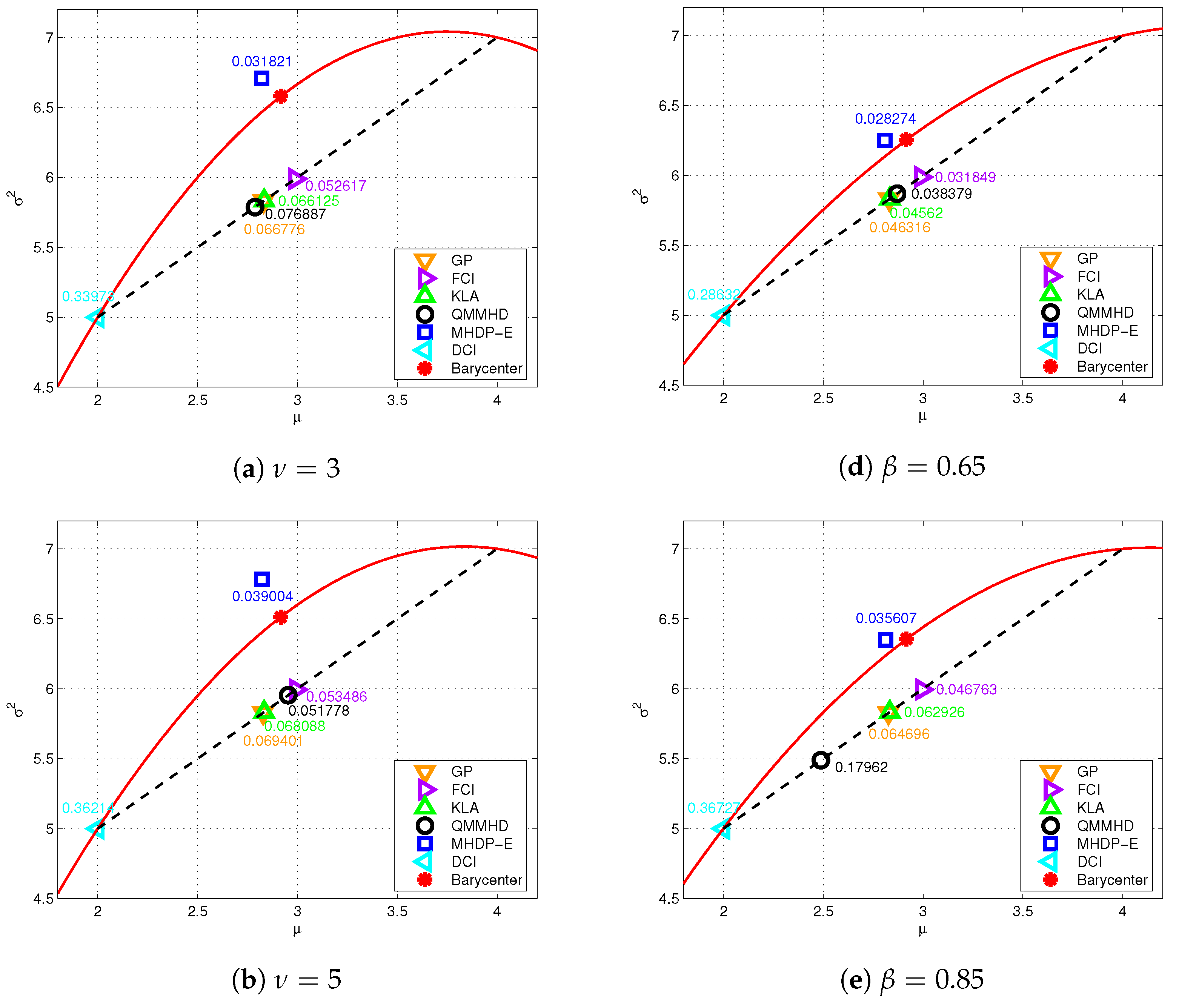
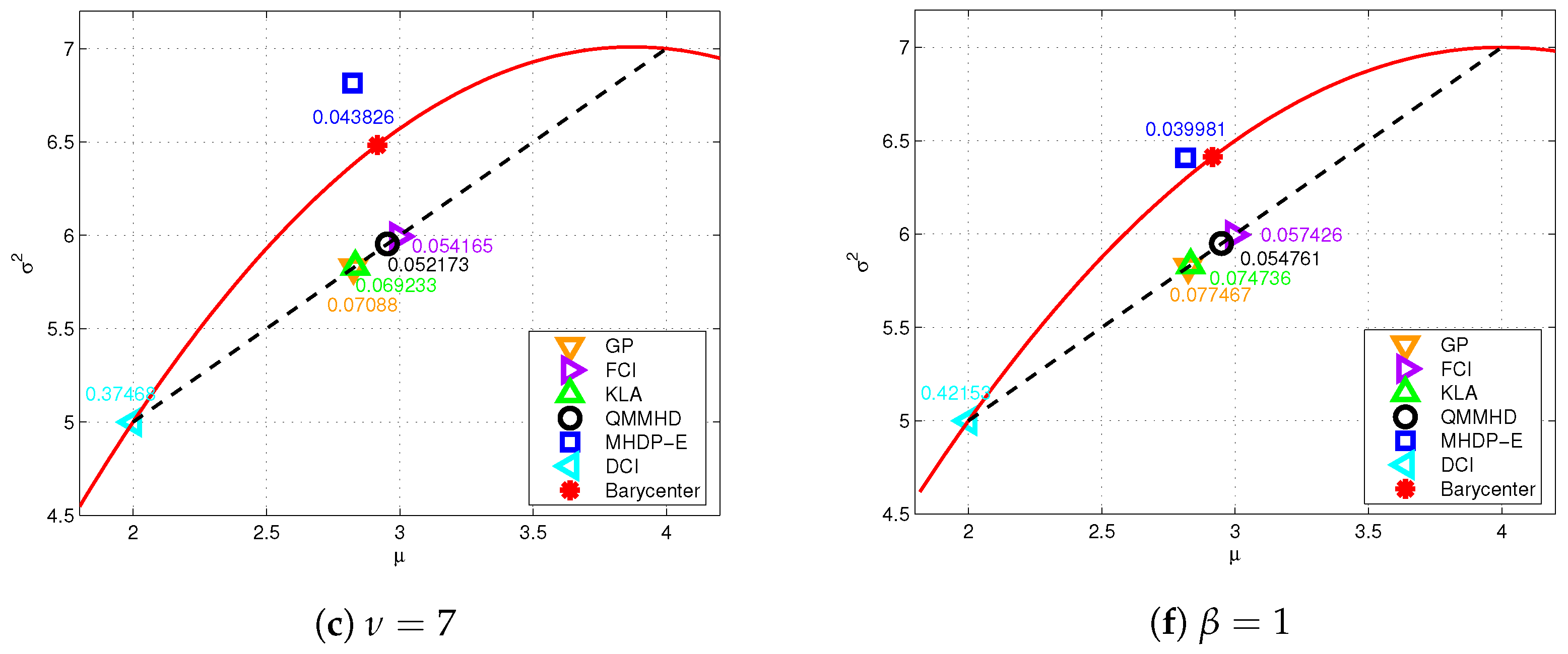
To intuitively evaluate the performance of these distributed fusion methods, we consider two local estimates and of a static target from two local sensors, similar to the settings in [42]. Note that the MHDP- I and MHDP-E methods have the same covariance fusion due to the commutability of two first-order matrices. In Figure 2, six subfigures are drawn to display the geodesic distance between the fused density and the informative barycenter under six different MED assumptions, respectively. Here, the informative barycenter as the optimal solution of (29) is an arbitrary point on the geodesic segment linking and , and we uniquely determine it by minimizing the sum of its squared distances to the two local estimates. Since the MHDP-I and MHDP-E are developed based on the relaxation of (29), learning about the informative barycenter can improve our understanding of their fusion performance as the heavy-tailed level varies.
- (i)
- The MTD has the degree of freedom (DOF) parameter (the higher , the lower the heavy-tailed level), and is almost equivalent to the Gaussian distribution as tends to infinity. As depicted in subfigures (a), (b) and (c), the MHDP-E is consistently superior to other methods regardless of the DOF, since the fused density of the MHDP-E is closest to the informative barycenter.
- (ii)
- The MGGD has the shape parameter (the higher , the lower the heavy-tailed level) and corresponds to the Gaussian distribution when . Similar to the MTD, subfigures (d), (e) and (f) show the MHDP-E outperforms other fusion methods for different shape parameters.
Moreover, the aforementioned fusion methods DCI, FCI, KLA, GP and QMMHD have the same form as (45), but with different weights in general. Thus in Figure 2 their fused estimates lie on the (straight) Euclidean segment between and , while the MHDP-E puts its estimate fairly close to the (curved) geodesic segment. Therefore, the MHDP-I and MHDP-E are considered more reasonable because the MED manifold is indeed non-Euclidean.
5.2. Dynamic Target Tracking
Consider a distributed dynamic system with n sensors and one fusion center for tracking a two-dimensional moving target:
where there are sensors for one-dimensional measurements and sensors for multi-dimensional measurements, the state vector consists of the position and velocity, and the sampling interval . As [49,50] for more practical scenarios, the outlier contaminated state and measurement noises are modeled as
where “w.p.” denotes “with probability”.
The local state estimate and scatter matrix of estimation error are computed by using the specified filter, when the i-th sensor obtains its own measurement at the instant k. The fusion center fuses all local estimates from the sensors to obtain the final estimate by applying some specified fusion methods, and then transmits it back to each local sensor. To demonstrate the performance of various fusion methods, i.e., the DCI, FCI, KLA, GP, QMMHD, MHDP-I and MHDP-E, we use the Student’s t based filter (STF) [49] and the Gaussian–Student’s t mixture distribution based Kalman filter (GSTMDKF) [41] to compare the root mean squared errors (RMSEs) of the fused results in the following two cases:
- (i)
- Case I (two sensors, i.e., ): The variances and , the measurement matricesand the two filters are initialized as
- (ii)
- Case II (three sensors, i.e., ): The system parameters have the same settings as Case I, and also
It is seen from (69)–(71) that the process and observation noises follow heavy-tailed distributions. The STF models the initial state vector and the noise distributions with as follows:
By (75)–(78), each local posterior density can be represented by the MTD with the DOF parameter , i.e., . In the GSTMDKF setup, a Gaussian–Student’s t mixture distribution (see [41] for more details) with the fixed DOF 3 is used to model the heavy-tailed noises (69)–(71) with , the initial state vector follows a Gaussian distribution, i.e., , and other parameters are the same as those in [41]. As explained in [41], the GSTM distribution has the same efficiency as the Student’s t distribution in the presence of outliers, and thus our proposed MHDP-E and MHDP-I methods fuse all posterior densities by modeling them as the MTDs with the common DOF parameter 3. Note that the DCI, FCI, KLA, and GP only utilize the first two moments (i.e., and for the i-th local posterior density), and the FCI, KLA and GP fusion methods are developed under Gaussian assumption so that the posterior density for the i-th sensor can be modeled as .
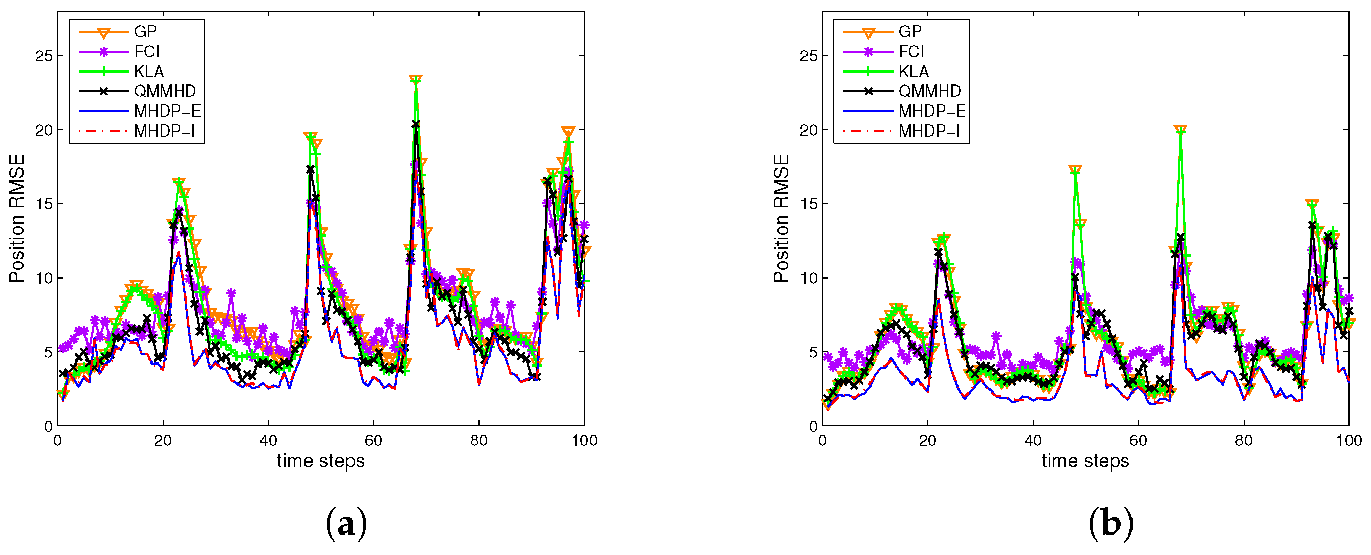
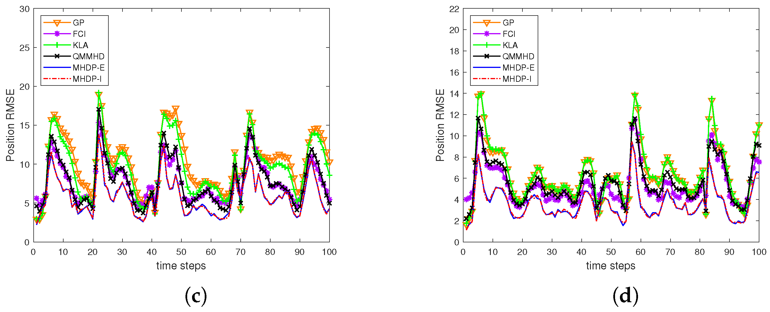
By adopting two different filters STF and GSTMDKF, Figure 3 shows the RMSEs of the position over 100 time steps and 500 Monte Carlo runs in two different cases using the aforementioned fusion methods, while the DCI does not appear in Figure 3 owing to it behaving worst. We can see that the proposed MHDP-I and MHDP-E are consistently better than other fusion methods when different filtering methods are adopted. Moreover, Table 1 reports the averaged root mean squared errors (ARMSEs) of the various methods in both cases. It is evident that the performance of all fusion methods in three-sensor example has a significant improvement over that in the two-sensor case, and also the MHDP-I performs slightly better than the MHDP-E when using the GSTMDKF. However in contrast to the MHDP-I, the MHDP-E has lower computational complexity due to the explicit expression for the fused covariance estimate.
6. Conclusions
In this work, we formulate an information-geometric fusion criterion, taking the geodesic distance as the loss function, and implement the fusion of local posterior densities on the MED manifold endowed with the Fisher metric. Two distributed estimation fusion algorithms MHDP-I and MHDP-E are proposed by using the minimal Manhattan distance instead of the geodesic distance on the manifold of MEDs, which both have the same mean estimation fusion, but differ in the form of covariance estimation fusion. On the MED submanifold with a fixed mean, the MHDP-I fuses all MHD-based projections of local posterior densities by minimizing the squared geodesic distances from a sought-for fused density. We have developed a robust fixed point iterative algorithm with theoretical convergence to compute the covariance estimate of such fused density. By introducing a specified Lie algebraic structure on the aforementioned submanifold and deriving its exponential and logarithmic mappings, the MHDP-E has provided an explicit expression for the fused covariance estimate. Numerical examples have shown better performance of the two proposed information-geometric methods than five other fusion methods.
Author Contributions
X.C. put forward the original ideas and conducted the research; J.Z. raised the research question, reviewed this paper and provided improvement suggestions. All authors have read and agreed to the published version of the manuscript.
Funding
This work was supported in part by the Sichuan Science and Technology Program under Grant 2022JDRC0068, and the National Natural Science Foundation of China under Grants 61374027, 11871357 and 12271376.
Acknowledgments
We thank the anonymous reviewers for their suggestions on improving the quality of this paper.
Conflicts of Interest
The authors declare no conflict of interest.
Appendix A. Proof of Theorem 1
Let and the variable transformation
By using (13), the geodesic equations on the MED manifold with the coordinate system can be rewritten as
Then, the squared line element along the geodesic becomes
Compared with (11), we obtain , where s is the arc length parameter before the transformation (A1). Therefore, by Theorem 6.5 in [62], the geodesic distance between and is given as
with . To that end, using Theorem 6.2 in [62], we obtain the geodesic curve on the MED manifold as
where and can be calculated by boundary conditions. Note that for the case of , the geodesic given by (15) and (16) are easily obtained by Equation (6.4) in [62].
Appendix B. Proof of Theorem 2
Appendix C. Proof of Theorem 3
Appendix D. Proof of Theorem 4
Define an auxiliary function
with . It is easy to know , and thus we have the inequality
for .
Appendix E. Proof of Theorem 5
Lemma A1
(See [52]). If is an invertible real matrix-valued function of real variable t and its eigenvalues lie on the positive real line, then
Let denote the geodesic emanating from the point at in an arbitrary direction . Inspired by the method in the proof of Lemma A1 in [52], we can easily know
Applying (A17) and (A18), and differentiating with respect to t, we have
where . As a result,
According to the arbitrariness of vector and the Riemannian inner product (23), we obtain the Riemannian gradient
Appendix F. Proof of Theorem 6
(i) From the inner product (23), we have the squared line element
By taking the congruent transformation , it is not difficult to see that the squared infinitesimal distance (A22) is invariant.
(ii) Suppose
where are the eigenvalues of . There exists a nonsingular matrix such that
where . According to the geodesic from to on
with initial conditions and (see [48]), we have , and then the geodesic direction
References
- Du, J.; Fang, M.; Yu, Y.; Lu, G. An adaptive two-scale biomedical image fusion method with statistical comparisons. Comput. Methods Programs Biomed. 2020, 196, 105603. [Google Scholar] [CrossRef] [PubMed]
- Zhao, F.; Zhao, W.; Yao, L.; Liu, Y. Self-supervised feature adaption for infrared and visible image fusion. Inf. Fusion 2021, 76, 189–203. [Google Scholar] [CrossRef]
- Shafran-Nathan, R.; Etzion, Y.; Broday, D. Fusion of land use regression modeling output and wireless distributed sensor network measurements into a high spatiotemporally-resolved NO2 product. Environ. Pollut. 2021, 271, 116334. [Google Scholar] [CrossRef]
- Xiao, K.; Wang, R.; Deng, H.; Zhang, L.; Yang, C. Energy-aware scheduling for information fusion in wireless sensor network surveillance. Inf. Fusion 2019, 48, 95–106. [Google Scholar] [CrossRef]
- Salcedo-Sanz, S.; Ghamisi, P.; Piles, M.; Werner, M.; Cuadra, L.; Moreno-Martínez, A.; Izquierdo-Verdiguier, E.; Muñoz-Marí, J.; Mosavi, A.; Camps-Valls, G. Machine learning information fusion in earth observation: A comprehensive review of methods, applications and data sources. Inf. Fusion 2020, 63, 256–272. [Google Scholar] [CrossRef]
- Liggins, M.E.; Hall, D.L.; Llinas, J. (Eds.) Handbook of Multisensor Data Fusion: Theory and Practice, 2nd ed.; CRC Press: Boca Raton, FL, USA, 2009. [Google Scholar]
- Li, G.; Battistelli, G.; Yi, W.; Kong, L. Distributed multi-sensor multi-view fusion based on generalized covariance intersection. Signal Process. 2020, 166, 107246. [Google Scholar] [CrossRef]
- Bar-Shalom, Y.; Campo, L. The effect of the common process noise on the two-sensor fused-track covariance. IEEE Trans. Aerosp. Electron. Syst. 1986, 22, 803–805. [Google Scholar] [CrossRef]
- Li, X.R.; Zhu, Y.; Wang, J.; Han, C. Optimal linear estimation fusion—Part I: Unified fusion rules. IEEE Trans. Inf. Theory 2003, 49, 2192–2208. [Google Scholar] [CrossRef]
- Julier, S.J.; Uhlmann, J.K. A non-divergent estimation algorithm in the presence of unknown correlations. In Proceedings of the 1997 American Control Conference, Albuquerque, NM, USA, 6 June 1997; pp. 2369–2373. [Google Scholar]
- Reinhardt, M.; Noack, B.; Arambel, P.O.; Hanebeck, U.D. Minimum covariance bounds for the fusion under unknown correlations. IEEE Signal Process. Lett. 2015, 22, 1210–1214. [Google Scholar] [CrossRef]
- Julier, S.J.; Uhlmann, J.K. General decentralized data fusion with covariance intersection (CI). In Handbook of Multisensor Data Fusion: Theory and Practice; CRC Press: Boca Raton, FL, USA, 2001; pp. 12.1–12.5. [Google Scholar]
- Chong, C.Y.; Mori, S. Convex combination and covariance intersection algorithms in distributed fusion. In Proceedings of the 4th International Conference of Information Fusion, Sun City, South Africa, 1–4 November 2001; Volume 1, pp. 11–18. [Google Scholar]
- Eldar, Y.C.; Beck, A.; Teboulle, M. A minimax Chebyshev estimator for bounded error estimation. IEEE Trans. Signal Process. 2008, 56, 1388–1397. [Google Scholar] [CrossRef]
- Wang, Y.; Li, X.R. Distributed estimation fusion under unknown cross-correlation: An analytic center approach. In Proceedings of the 13th International Conference on Information Fusion, Edinburgh, UK, 26–29 July 2010; pp. 1–8. [Google Scholar]
- Hurley, M.B. An information theoretic justification for covariance intersection and its generalization. In Proceedings of the 5th International Conference on Information Fusion, Annapolis, MA, USA, 8–11 July 2002; pp. 505–511. [Google Scholar]
- Wang, Y.; Li, X.R. A fast and fault-tolerant convex combination fusion algorithm under unknown cross-correlation. In Proceedings of the 12th International Conference on Information Fusion, Seattle, WA, USA, 6–9 July 2009; pp. 571–578. [Google Scholar]
- Battistelli, G.; Chisci, L. Kullback–Leibler average, consensus on probability densities, and distributed state estimation with guaranteed stability. Automatica 2014, 50, 707–718. [Google Scholar] [CrossRef]
- Costa, S.I.R.; Santos, S.A.; Strapasson, J.E. Fisher information distance: A geometrical reading. Discret. Appl. Math. 2015, 197, 59–69. [Google Scholar] [CrossRef]
- Bishop, A.N. Information fusion via the Wasserstein barycenter in the space of probability measures: Direct fusion of empirical measures and Gaussian fusion with unknown correlation. In Proceedings of the 17th International Conference on Information Fusion, Salamanca, Spain, 7–10 July 2014; pp. 1–7. [Google Scholar]
- Takatsu, A. Wasserstein geometry of Gaussian measures. Osaka J. Math. 2011, 48, 1005–1026. [Google Scholar]
- Puccetti, G.; Rüschendorf, L.; Vanduffel, S. On the computation of Wasserstein barycenters. J. Multivar. Anal. 2020, 176, 104581. [Google Scholar] [CrossRef]
- Amari, S.I.; Kurata, K.; Nagaoka, H. Information geometry of Boltzmann machines. IEEE Trans. Neural Netw. 1992, 3, 260–271. [Google Scholar] [CrossRef]
- Amari, S.I. Information geometry of the EM and em algorithms for neural networks. Neural Netw. 1995, 8, 1379–1408. [Google Scholar] [CrossRef]
- Cheng, Y.; Wang, X.; Morelande, M.; Moran, B. Information geometry of target tracking sensor networks. Inf. Fusion 2013, 14, 311–326. [Google Scholar] [CrossRef]
- Eilders, M.J. Decentralized Riemannian Particle Filtering with Applications to Multi-Agent Localization. Ph.D. Thesis, Air Force Institute of Technology, Dayton, OH, USA, 2012. [Google Scholar]
- Amari, S.I.; Kawanabe, M. Information geometry of estimating functions in semi-parametric statistical models. Bernoulli 1997, 3, 29–54. [Google Scholar] [CrossRef]
- Rong, Y.; Tang, M.; Zhou, J. Intrinsic losses based on information geometry and their applications. Entropy 2017, 19, 405. [Google Scholar] [CrossRef] [Green Version]
- Gómez, E.; Gomez-Viilegas, M.A.; Marín, J.M. A multivariate generalization of the power exponential family of distributions. Commun. Stat.–Theory Methods 1998, 27, 589–600. [Google Scholar] [CrossRef]
- Samuel, K. Multivariate t-Distributions and Their Applications; Cambridge University Press: Cambridge, UK, 2004. [Google Scholar]
- Kotz, S.; Kozubowski, T.J.; Podgórski, K. (Eds.) The Laplace Distribution and Generalizations: A Revisit with Applications to Communications, Economics, Engineering, and Finance; Birkhäuser: Boston, MA, USA, 2001. [Google Scholar]
- Wen, C.; Cheng, X.; Xu, D. Filter design based on characteristic functions for one class of multi-dimensional nonlinear non-Gaussian systems. Automatica 2017, 82, 171–180. [Google Scholar] [CrossRef]
- Chen, B.; Liu, X.; Zhao, H.; Príncipe, J.C. Maximum correntropy Kalman filter. Automatica 2017, 76, 70–77. [Google Scholar] [CrossRef] [Green Version]
- Agamennoni, G.; Nieto, J.I.; Nebot, E.M. Approximate inference in state-space models with heavy-tailed noise. IEEE Trans. Signal Process. 2012, 60, 5024–5037. [Google Scholar] [CrossRef]
- Do, M.N.; Vetterli, M. Wavelet-based texture retrieval using generalized Gaussian density and Kullback–Leibler distance. IEEE Trans. Image Process. 2002, 11, 146–158. [Google Scholar] [CrossRef] [Green Version]
- Tzagkarakis, G.; Beferull-Lozano, B.; Tsakalides, P. Rotation-invariant texture retrieval with Gaussianized steerable pyramids. IEEE Trans. Image Process. 2006, 15, 2702–2718. [Google Scholar] [CrossRef] [PubMed] [Green Version]
- Verdoolaege, G.; Scheunders, P. Geodesics on the manifold of multivariate generalized Gaussian distributions with an application to multicomponent texture discrimination. Int. J. Comput. Vis. 2011, 95, 265–286. [Google Scholar] [CrossRef] [Green Version]
- Xue, C.; Huang, Y.; Zhu, F.; Zhang, Y.; Chambers, J.A. An outlier-robust Kalman filter with adaptive selection of elliptically contoured distributions. IEEE Trans. Signal Process. 2022, 70, 994–1009. [Google Scholar] [CrossRef]
- Huang, Y.; Zhang, Y.; Zhao, Y.; Chambers, J.A. A novel outlier-robust Kalman filtering framework based on statistical similarity measure. IEEE Trans. Signal Process. 2021, 66, 2677–2692. [Google Scholar] [CrossRef]
- Zhu, F.; Huang, Y.; Xue, C.; Mihaylova, L.; Chambers, J.A. A sliding window variational outlier-robust Kalman filter based on Student’s t noise modelling. IEEE Trans. Signal Process. 2022, 58, 4835–4849. [Google Scholar]
- Huang, Y.; Zhang, Y.; Zhao, Y.; Chambers, J.A. A novel robust Gaussian–Student’s t mixture distribution based Kalman filter. IEEE Trans. Signal Process. 2019, 67, 3606–3620. [Google Scholar] [CrossRef]
- Tang, M.; Rong, Y.; Zhou, J.; Li, X.R. Information geometric approach to multisensor estimation fusion. IEEE Trans. Signal Process. 2019, 67, 279–292. [Google Scholar] [CrossRef]
- Chen, X.; Zhou, J.; Hu, S. Upper bounds for Rao distance on the manifold of multivariate elliptical distributions. Automatica 2021, 129, 109604. [Google Scholar] [CrossRef]
- Amari, S.I.; Nagaoka, H. Methods of Information Geometry; American Mathematical Society: Providence, RI, USA, 2000. [Google Scholar]
- Absil, P.A.; Mahony, R.; Sepulchre, R. Optimization Algorithms on Matrix Manifolds; Princeton University Press: Princeton, NJ, USA, 2009. [Google Scholar]
- Mitchell, A.F.S. The information matrix, skewness tensor and α-connections for the general multivariate elliptic distribution. Ann. Inst. Stat. Math. 1989, 41, 289–304. [Google Scholar] [CrossRef]
- Calvo, M.; Oller, J.M. A distance between elliptical distributions based in an embedding into the Siegel group. J. Comput. Appl. Math. 2002, 145, 319–334. [Google Scholar] [CrossRef] [Green Version]
- Berkane, M.; Oden, K.; Bentler, P.M. Geodesic estimation in elliptical distributions. J. Multivar. Anal. 1997, 63, 35–46. [Google Scholar] [CrossRef] [Green Version]
- Huang, Y.; Zhang, Y.; Ning, L.; Chambers, J.A. Robust Student’s t based nonlinear filter and smoother. IEEE Trans. Aerosp. Electron. Syst. 2016, 52, 2586–2596. [Google Scholar] [CrossRef] [Green Version]
- Huang, Y.; Zhang, Y.; Chambers, J.A. A novel Kullback–Leibler divergence minimization-based adaptive Student’s t-filter. IEEE Trans. Signal Process. 2019, 67, 5417–5432. [Google Scholar] [CrossRef]
- Schweppe, F.C. Uncertain Dynamic Systems; Prentice Hall: Englewood Cliffs, NJ, USA, 1973. [Google Scholar]
- Moakher, M. A differential geometric approach to the geometric mean of symmetric positive-definite matrices. SIAM J. Matrix Anal. Appl. 2005, 26, 735–747. [Google Scholar] [CrossRef] [Green Version]
- Said, S.; Bombrun, L.; Berthoumieu, Y.; Manton, J.H. Riemannian Gaussian distributions on the space of symmetric positive definite matrices. IEEE Trans. Inf. Theory 2017, 63, 2153–2170. [Google Scholar] [CrossRef] [Green Version]
- Ilea, I.; Bombrun, L.; Terebes, R.; Borda, M.; Germain, C. An M-estimator for robust centroid estimation on the manifold of covariance matrices. IEEE Signal Process. Lett. 2016, 23, 1255–1259. [Google Scholar] [CrossRef] [Green Version]
- Fletcher, P.T.; Venkatasubramanian, S.; Joshi, S. The geometric median on Riemannian manifolds with application to robust atlas estimation. Neuroimage 2009, 45, S143–S152. [Google Scholar] [CrossRef] [Green Version]
- Hajri, H.; Ilea, I.; Said, S.; Bombrun, L.; Berthoumieu, Y. Riemannian Laplace distribution on the space of symmetric positive definite matrices. Entropy 2016, 18, 98. [Google Scholar] [CrossRef]
- Arnaudon, M.; Barbaresco, F.; Yang, L. Riemannian medians and means with applications to radar signal processing. IEEE J. Sel. Top. Signal Process. 2013, 7, 595–604. [Google Scholar] [CrossRef]
- Wong, K.M.; Zhang, J.K.; Liang, J.; Jiang, H. Mean and median of PSD matrices on a Riemannian manifold: Application to detection of narrow-band sonar signals. IEEE Trans. Signal Process. 2017, 65, 6536–6550. [Google Scholar] [CrossRef] [Green Version]
- Grove, K.; Karcher, H.; Ruh, E. Jacobi fields and Finsler metrics on compact Lie groups with an application to differentiable pinching problems. Math. Ann. 1974, 211, 7–21. [Google Scholar] [CrossRef]
- Arsigny, V.; Fillard, P.; Pennec, X.; Ayache, N. Geometric means in a novel vector space structure on symmetric positive-definite matrices. SIAM J. Matrix Anal. Appl. 2007, 29, 328–347. [Google Scholar] [CrossRef] [Green Version]
- Li, P.; Wang, Q.; Zeng, H.; Zhang, L. Local log-Euclidean multivariate Gaussian descriptor and its application to image classification. IEEE Trans. Pattern Anal. Mach. Intell. 2017, 39, 803–817. [Google Scholar] [CrossRef]
- Skovgaard, L.T. A Riemannian geometry of the multivariate normal model. Scand. J. Stat. 1984, 11, 211–223. [Google Scholar]
- Hunter, D.R.; Lange, K. A tutorial on MM algorithms. Am. Stat. 2004, 58, 30–37. [Google Scholar] [CrossRef]
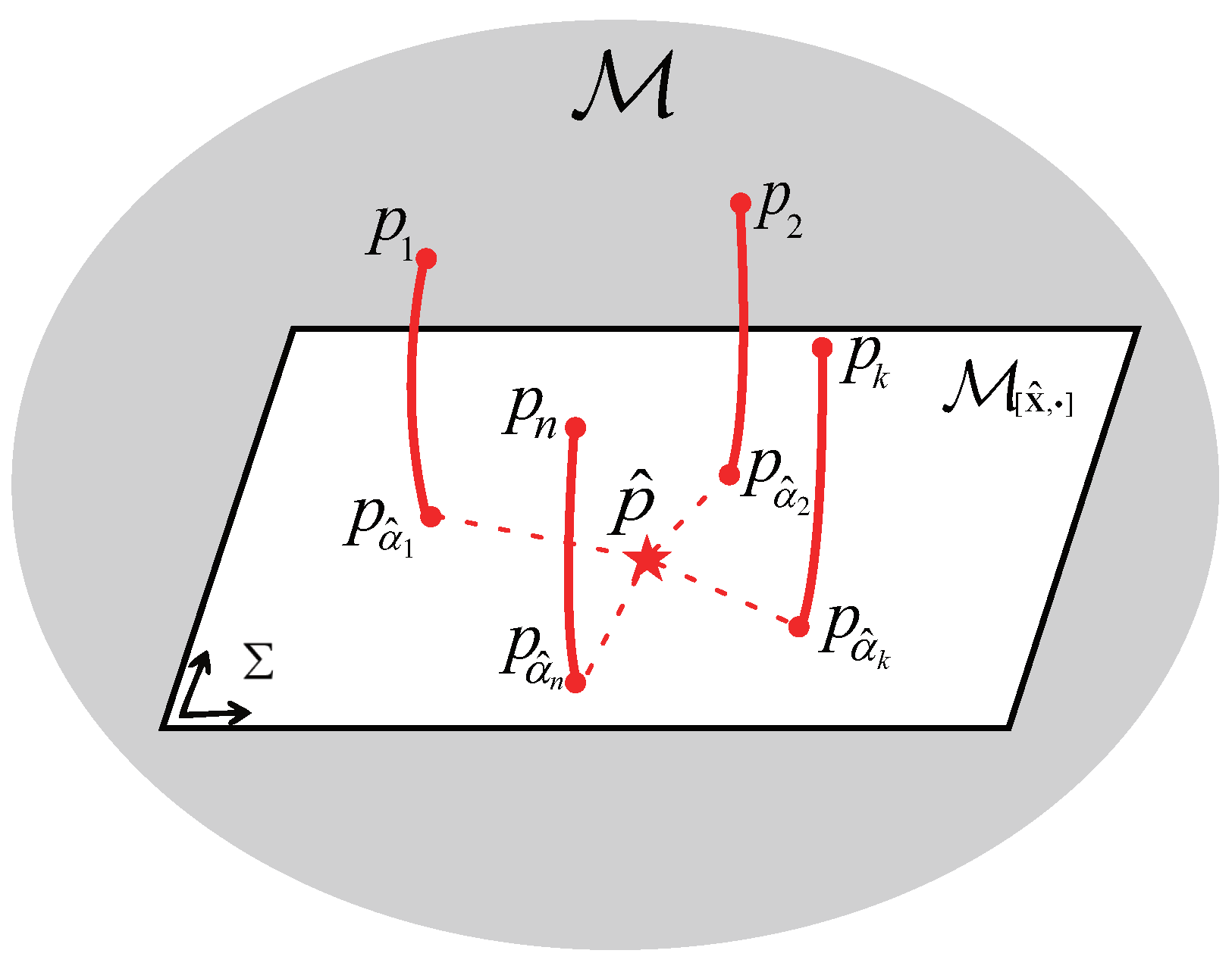
Figure 1.
The fusion of n local posterior densities based on the MHDPs.

Figure 2.
Six subfigures are depicted for the geodesic distance between the fused density and the informative barycenter. The various fused results are labeled by the specified marks. Subfigures (a–c) correspond to MTDs with DOF parameters and 7, respectively. Subfigures (d–f) correspond to MGGDs with shape parameters and 1, respectively. In each subfigure, the geodesic distances between the informative barycenter and the fused densities are displayed, and the geodesic between the two local densities is represented by the solid red curve.


Figure 3.
The position RMSEs of fused results vs. the instant k from 1 to 100 by (a) the STF in Case I; (b) the STF in Case II; (c) the GSTMDKF in Case I; and (d) the GSTMDKF in Case II.
Figure 3.
The position RMSEs of fused results vs. the instant k from 1 to 100 by (a) the STF in Case I; (b) the STF in Case II; (c) the GSTMDKF in Case I; and (d) the GSTMDKF in Case II.


Table 1.
The Position ARMSEs of seven fusion methods in both cases by the STF and the GSTMDKF.
| Method | STF | GSTMDKF | ||
|---|---|---|---|---|
| Case I | Case II | Case I | Case II | |
| DCI | ||||
| GP | ||||
| FCI | ||||
| KLA | ||||
| QMMHD | ||||
| MHDP-E | ||||
| MHDP-I | ||||
Publisher’s Note: MDPI stays neutral with regard to jurisdictional claims in published maps and institutional affiliations. |
© 2022 by the authors. Licensee MDPI, Basel, Switzerland. This article is an open access article distributed under the terms and conditions of the Creative Commons Attribution (CC BY) license (https://creativecommons.org/licenses/by/4.0/).
Share and Cite
MDPI and ACS Style
Chen, X.; Zhou, J. Multisensor Estimation Fusion on Statistical Manifold. Entropy 2022, 24, 1802. https://doi.org/10.3390/e24121802
AMA Style
Chen X, Zhou J. Multisensor Estimation Fusion on Statistical Manifold. Entropy. 2022; 24(12):1802. https://doi.org/10.3390/e24121802
Chicago/Turabian StyleChen, Xiangbing, and Jie Zhou. 2022. "Multisensor Estimation Fusion on Statistical Manifold" Entropy 24, no. 12: 1802. https://doi.org/10.3390/e24121802
Note that from the first issue of 2016, this journal uses article numbers instead of page numbers. See further details here.