
Variational Quantum Algorithm Applied to Collision Avoidance of Unmanned Aerial Vehicles

Abstract
:1. Introduction
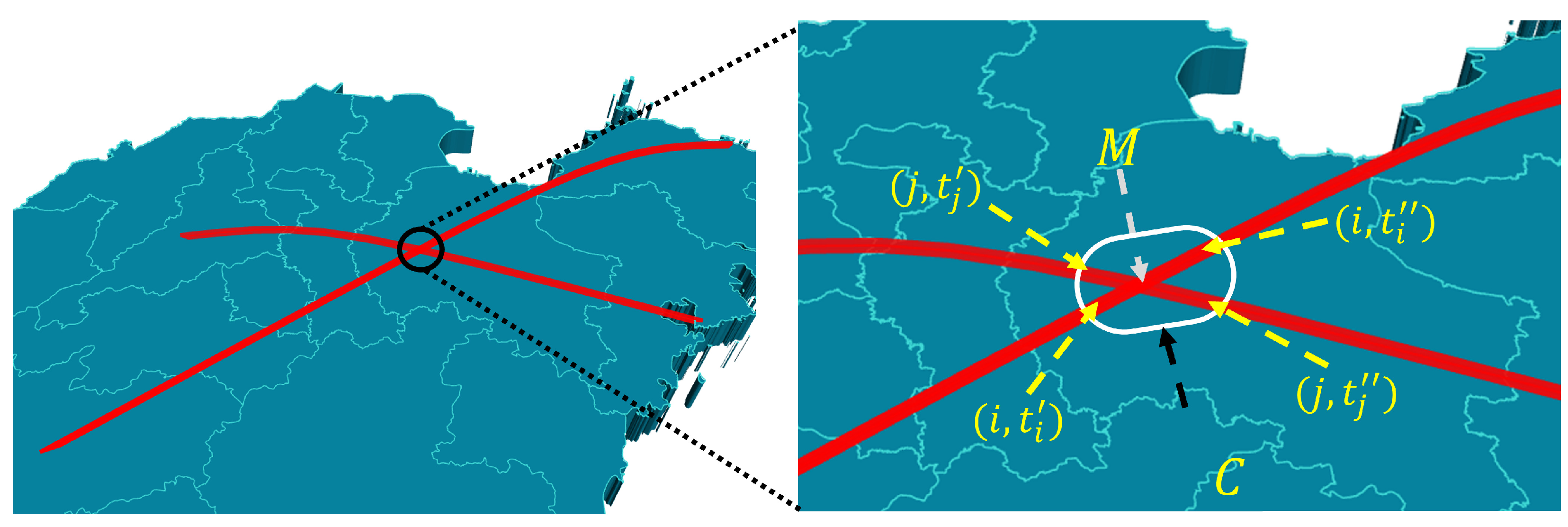
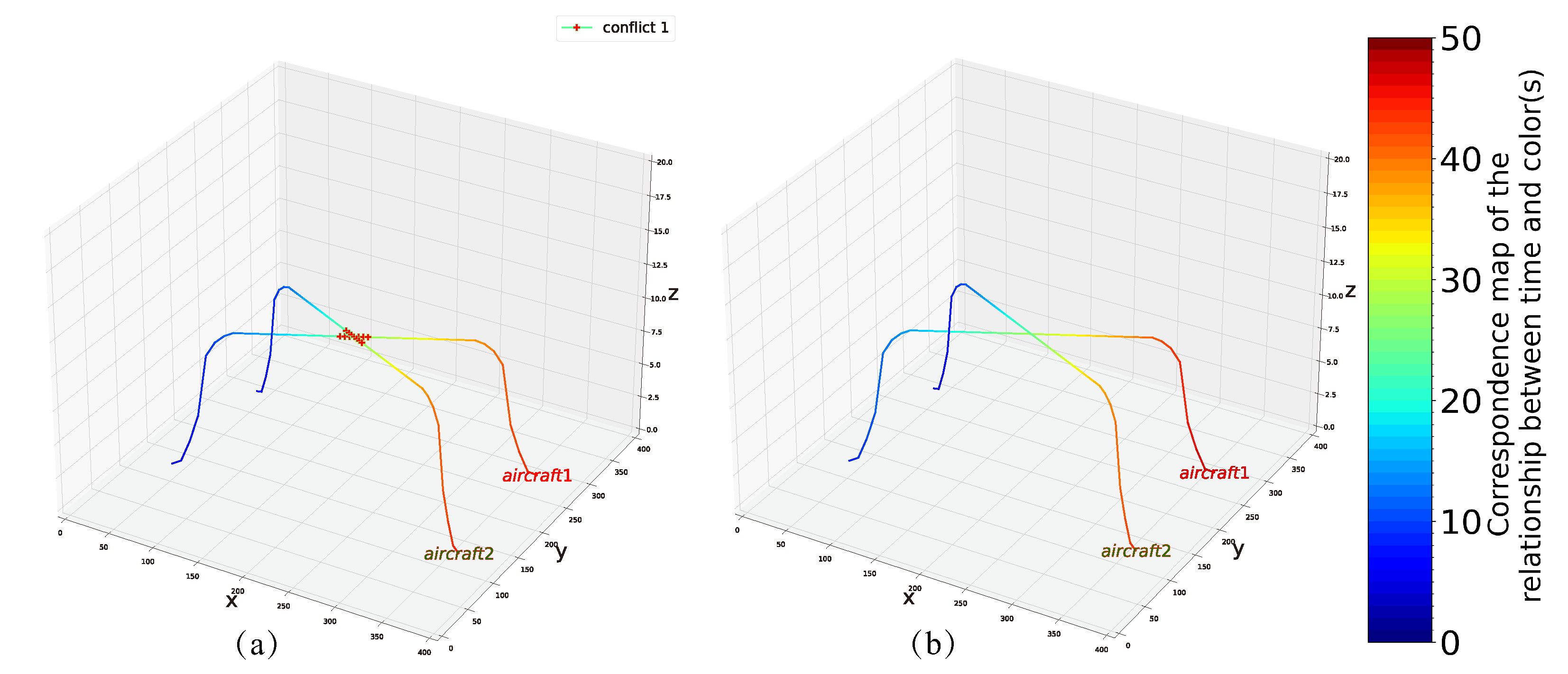
- Spatio-temporal conditions. For the objective requirement of the aircraft to ensure safety of flight, the distance between any two aircraft at the same point in time must be greater than a threshold value. From the standpoint of flight tasks, this requires us to adjust the trajectory of the aircraft or change the time of arrival at the conflict point when a conflict occurs. If we put it in mathematical perspective, it means that we must ensure that, for at least one of the two, the spatial function A and the temporal function T, should be bigger than 0.
- Preparation condition. Because of the special features of UAVs, the aircraft require preparation before takeoff. Nevertheless, the preparation time needed before takeoff is different for various types of aircraft, so we set a non-negative extra time for each aircraft, which is named pre-takeoff preparation time.
- Early takeoff condition. Unlike civil flights carrying people, in the mission of the UAVs we allow aircraft to take off earlier than scheduled departure time in order to avoid conflicts. This means that the departure delay time of the aircraft can not only be positive but also be negative.
- Heterogeneity condition. A UAV formation has different types and different models of aircraft that are required to perform different missions. For the priority of the aircraft resulting from the importance of missions to be performed or the urgency of tasks to be executed, we assign corresponding weights to each aircraft.
2. UAV Collision Avoidance Theory
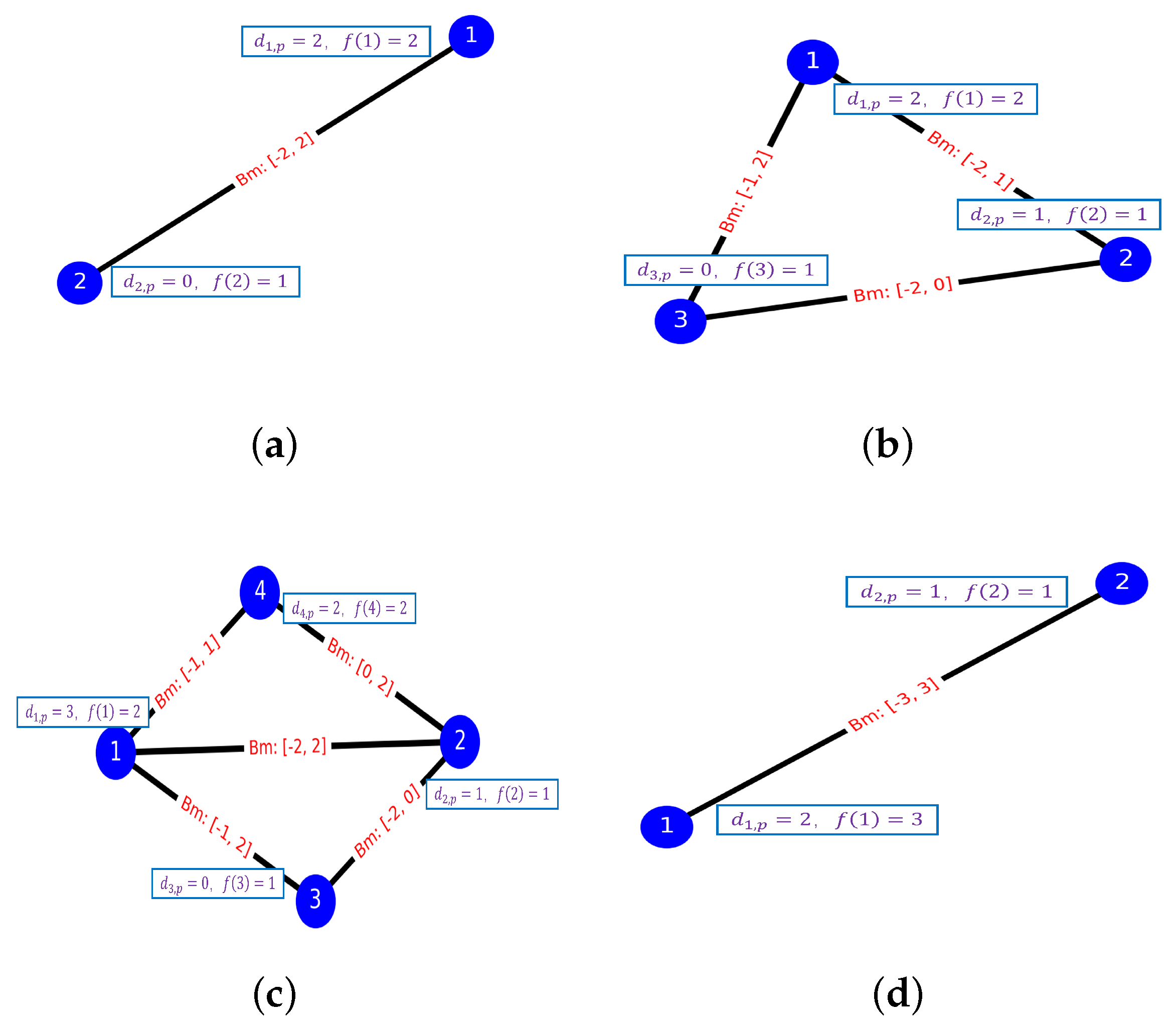
2.1. Problem Description
2.2. Mapping Problem to QUBO
3. Ising Model and Variational Quantum Algorithm
3.1. Ising Model and QUBO Problem
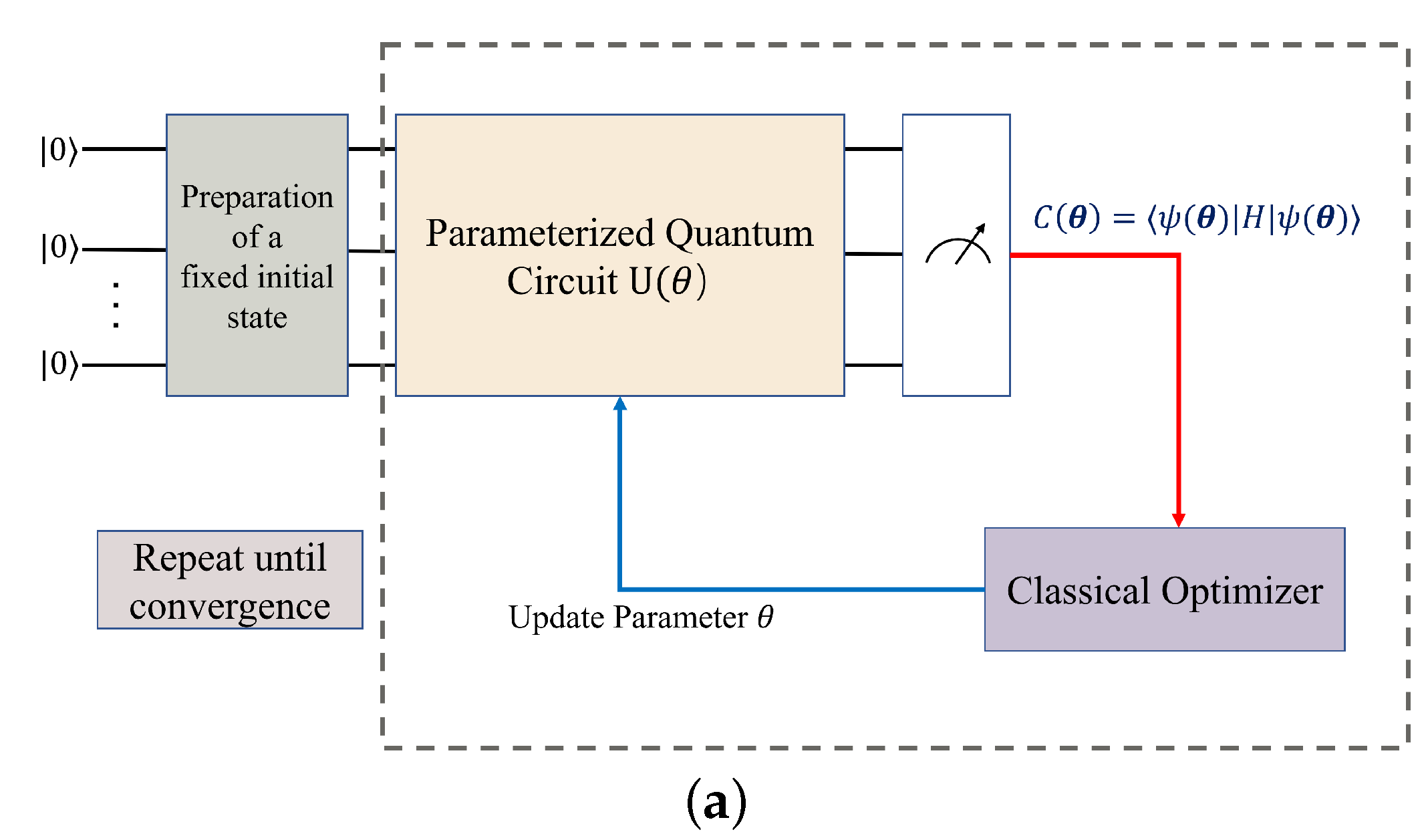
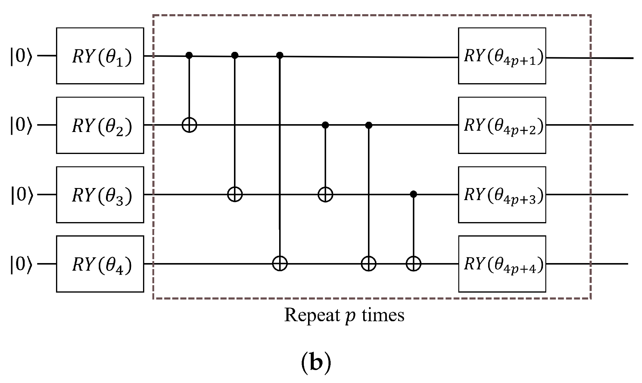
3.2. Variational Quantum Eigensolver (VQE)
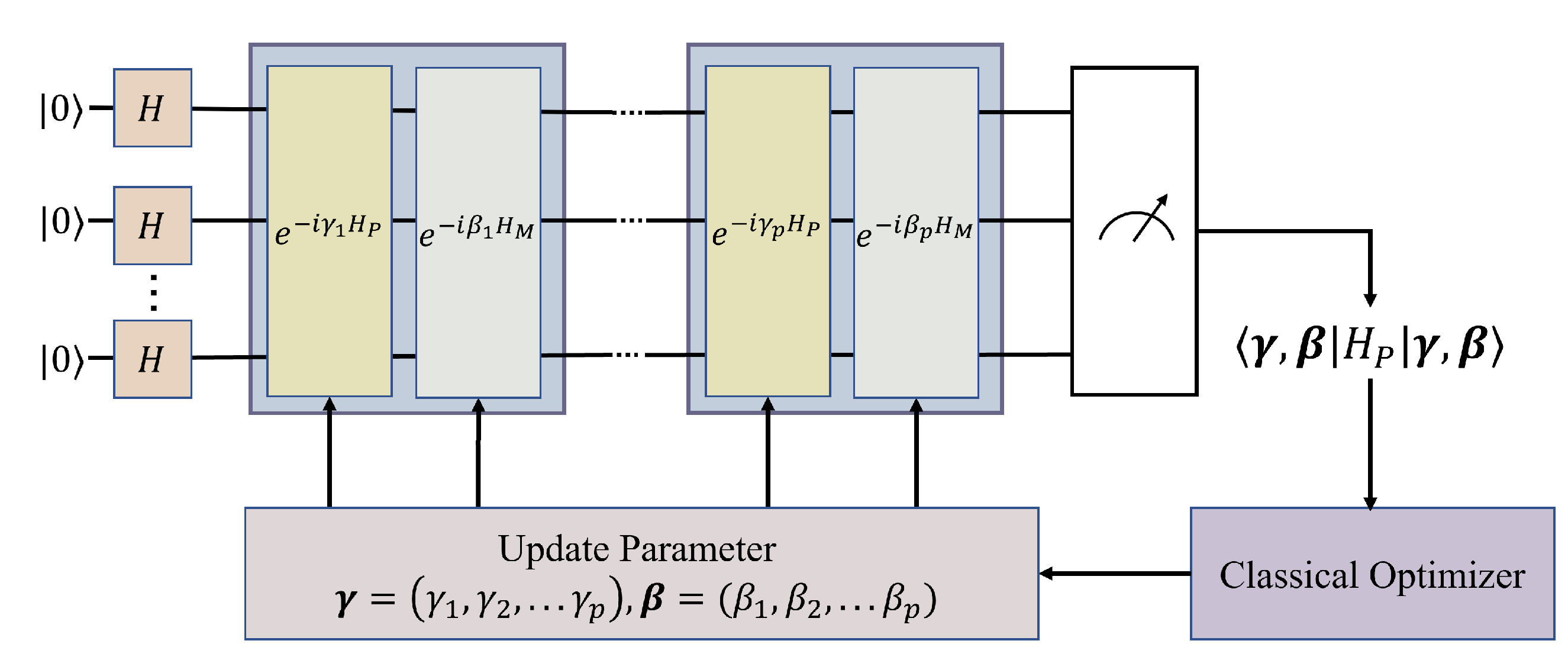
3.3. Quantum Approximate Optimization Algorithms
3.4. Conditional Value-at-Risk
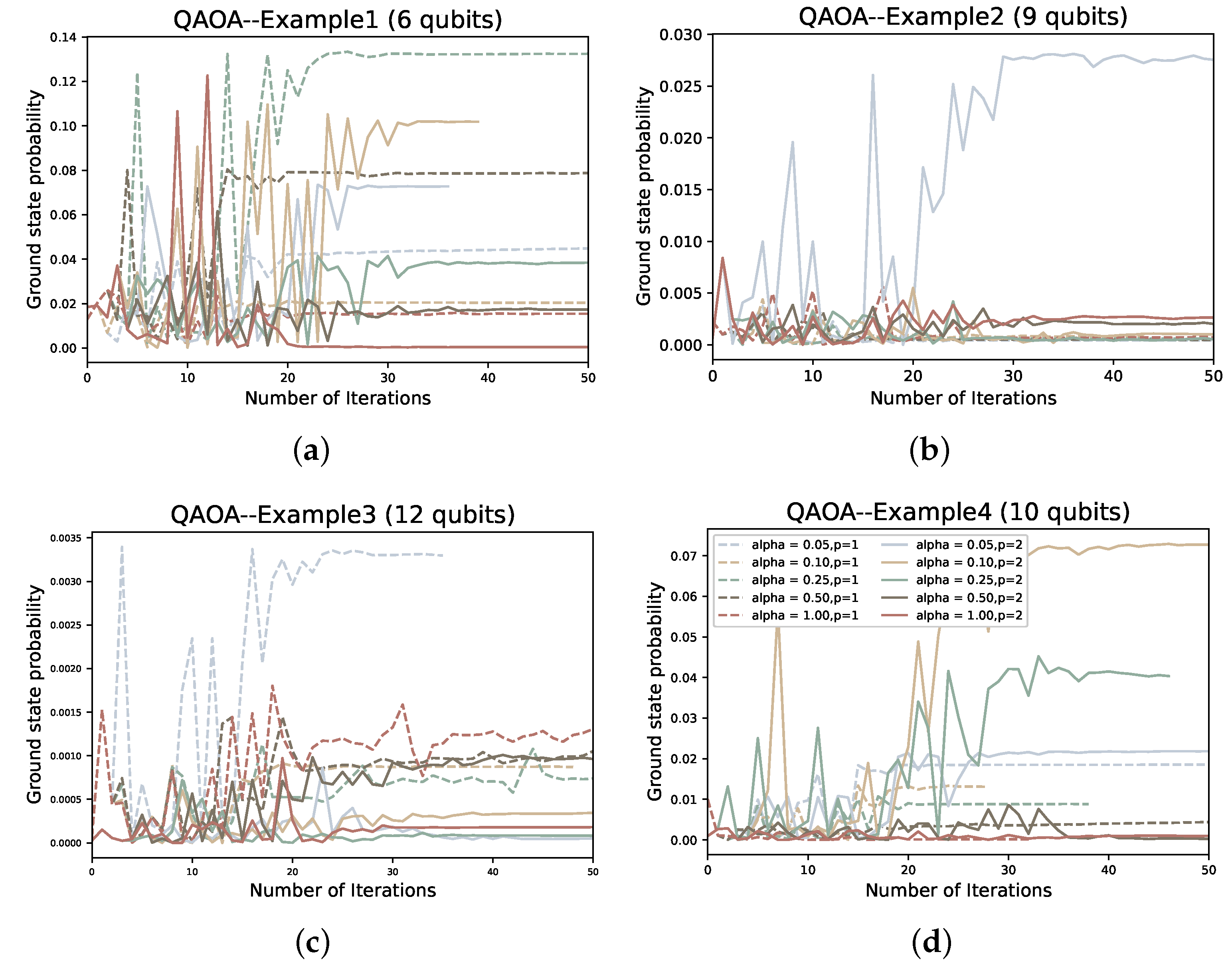
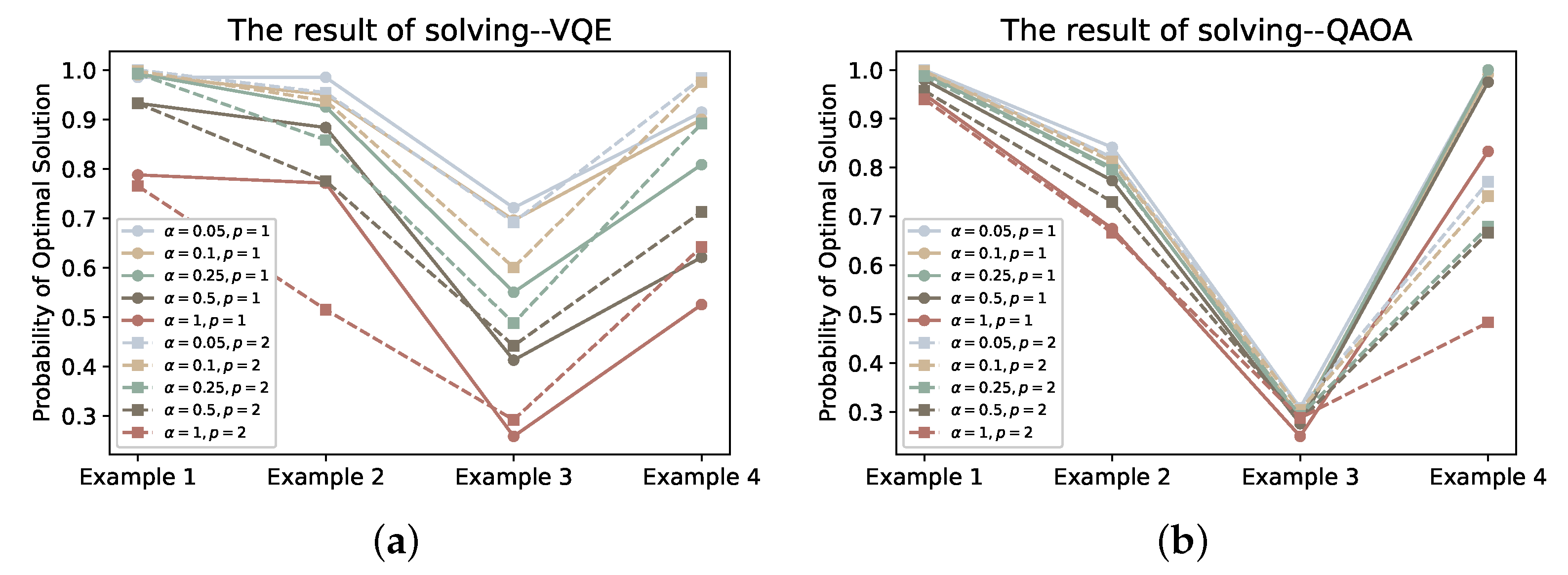
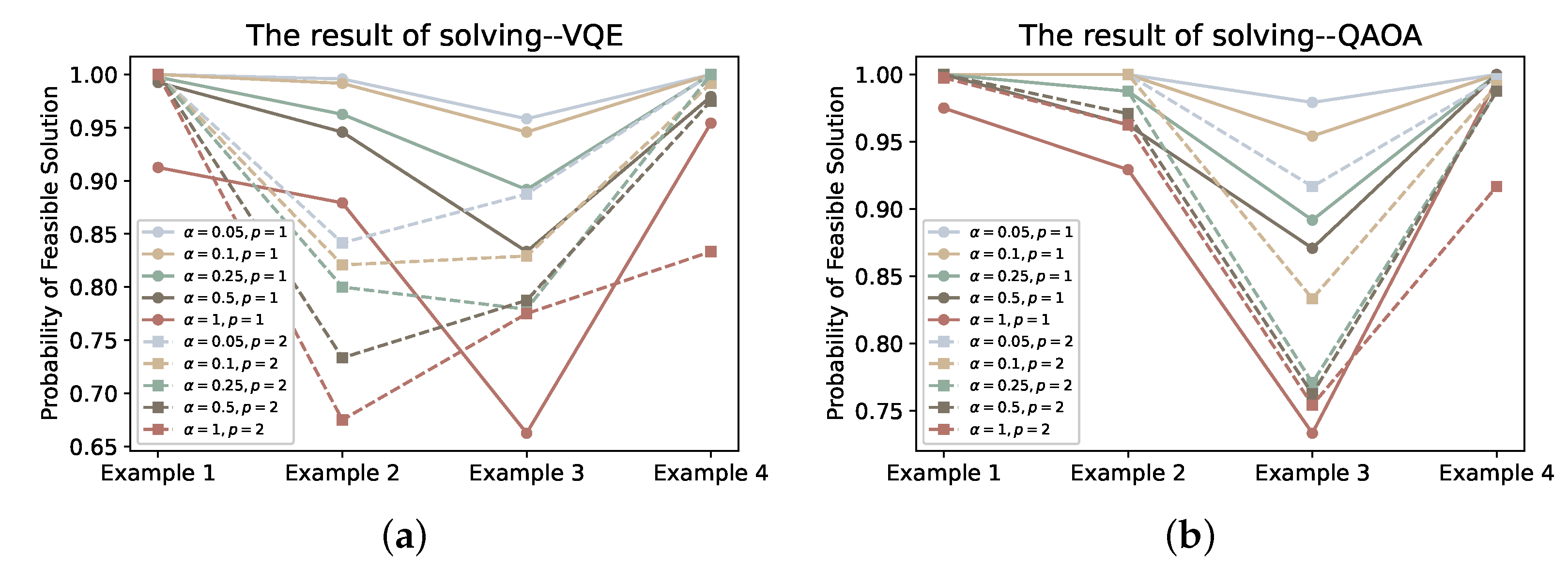
4. Result
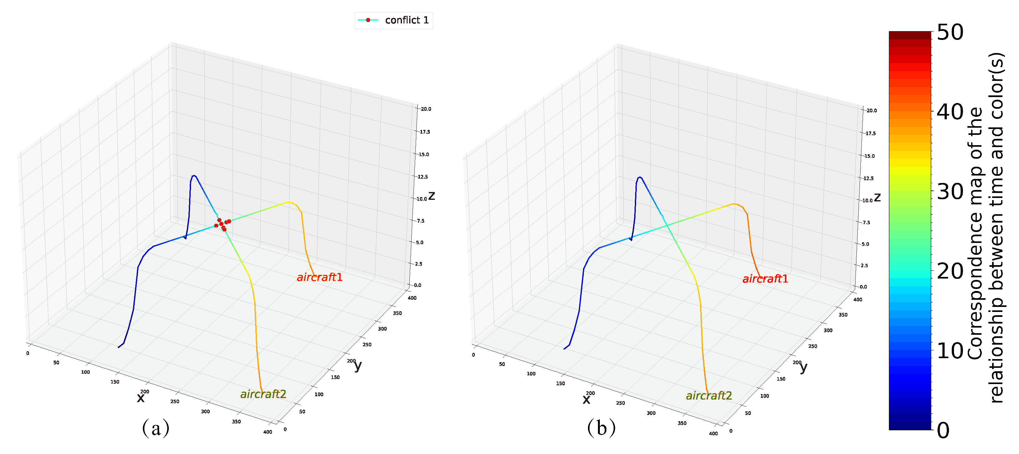
4.1. Example 1
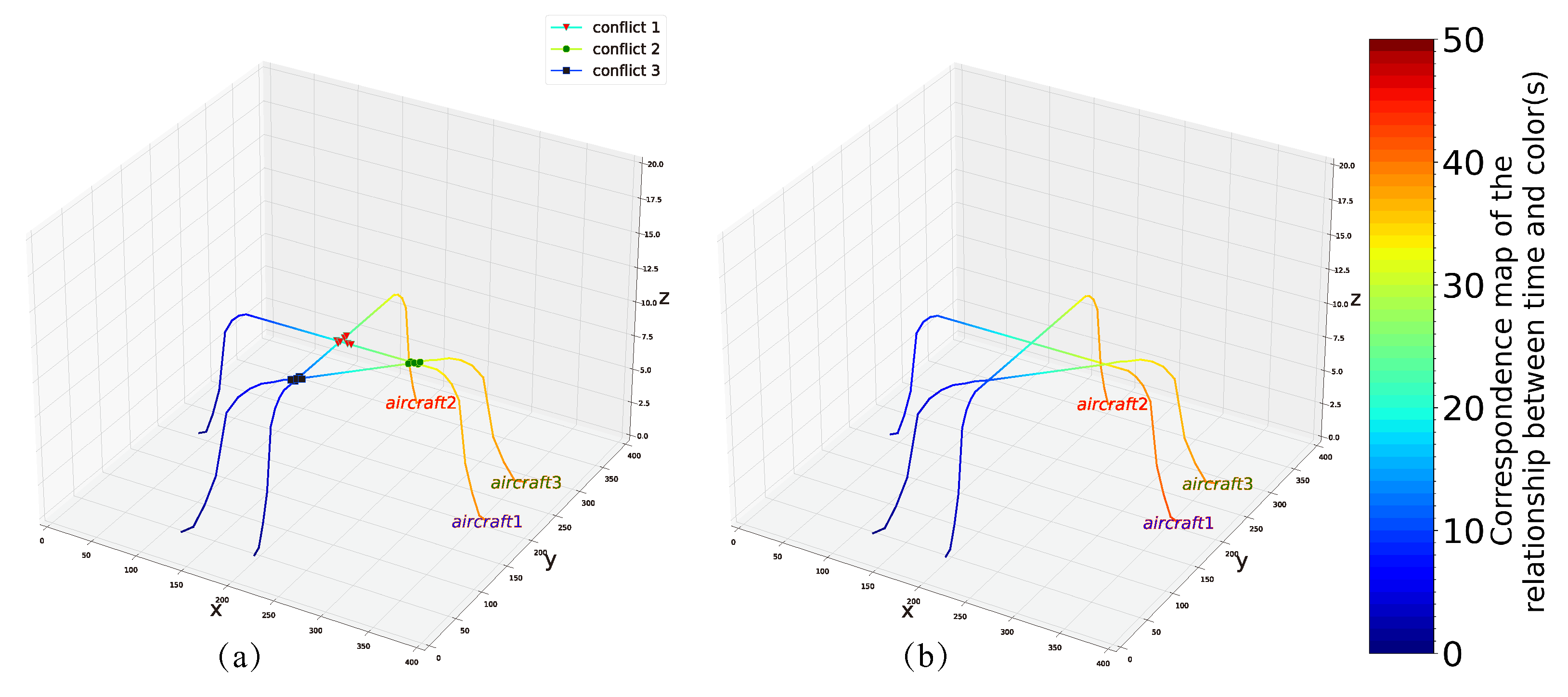
4.2. Example 2
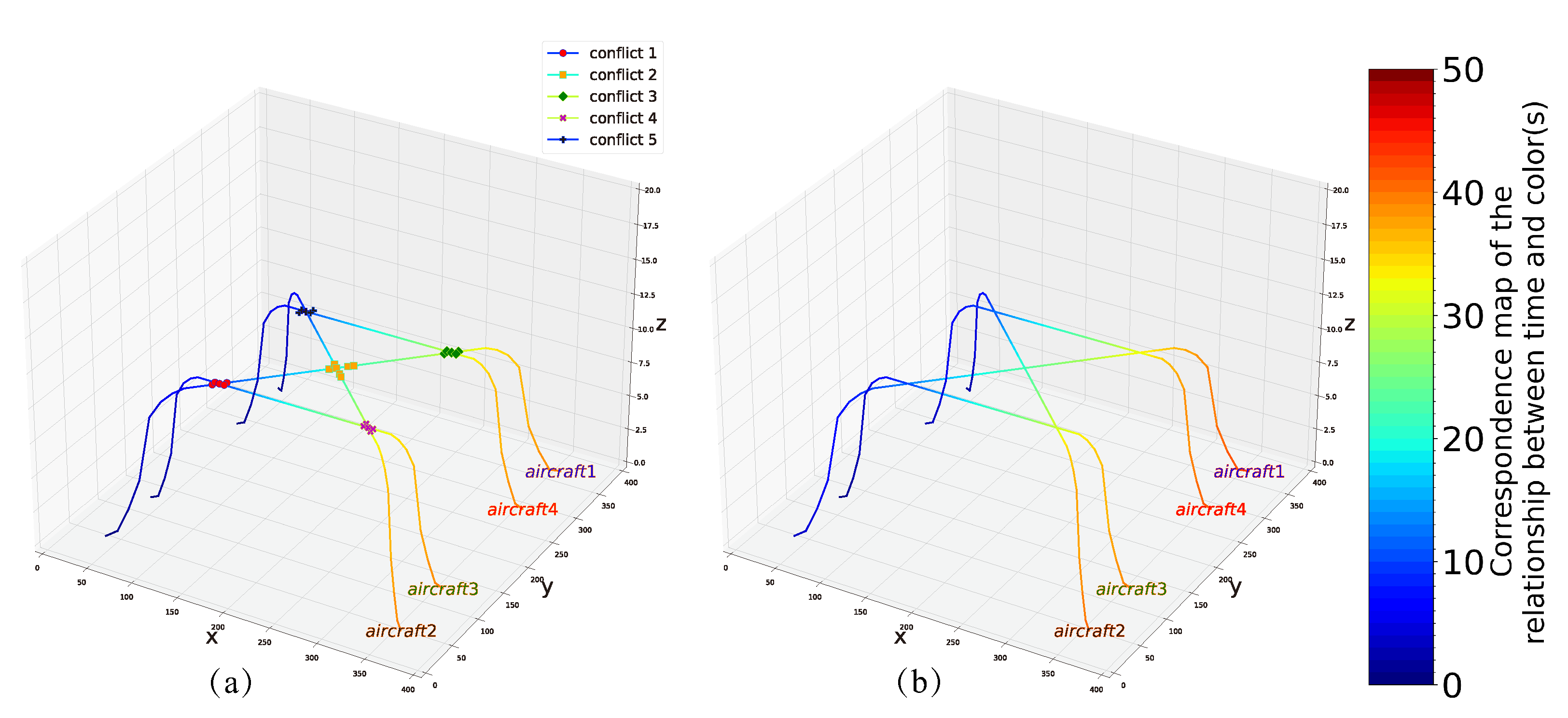
4.3. Example 3
4.4. Example 4
5. Conclusions
- In model building, the main consideration of this paper is to avoid collision by extending the aircraft takeoff time. In a real situation, in order to extend the usability of the model, we can also consider making some adjustments to the flight path to avoid collision, including changing the flight speed in a specific interval and partially changing the flight path of the aircraft, etc. These strategies can be collectively referred to as maneuvering collision avoidance strategies. We can adjust the cost function of the model by mapping the maneuver cost to the time delay cost in conjunction with the actual demand.
- In the aspect of quantum computing, on the one hand, in order to improve the efficiency of model solving, we can use more efficient coding methods to reduce the number of qubits required and the depth of quantum circuits to compress the time to solve the problem when encoding the decision variables. However, this requires us to modify the mapping between the model and the QUBO problem. Second, from the algorithmic point of view, improving the classical optimizer or adopting a more efficient ansatz structure is also an effective way to improve the efficiency of the algorithm.
Author Contributions
Funding
Institutional Review Board Statement
Informed Consent Statement
Data Availability Statement
Conflicts of Interest
Abbreviations
| VQA | Variational Quantum Algorithms |
| VQE | Variational Quantum Eigensolver |
| QAOA | Quantum Approximate Optimization Algorithm |
| QUBO | Quadratic Unconstrained Binary Optimization |
| ATM | Air Traffic Management |
| ATFM | Air Traffic Flow Management |
| UAV | Unmanned Aerial Vehicles |
| UTM | Unmanned Traffic Management |
| NISQ | Noisy Intermediate-Scale Quantum |
| CVaR | Conditional Value-at-Risk |
| UAM | Urban Air Mobility |
| NASA | National Aeronautics and Space Administration |
| PQC | Parameterized Quantum Circuits |
References
- Hildmann, H.; Kovacs, E. Using unmanned aerial vehicles (UAVs) as mobile sensing platforms (MSPs) for disaster response, civil security and public safety. Drones 2019, 3, 59. [Google Scholar] [CrossRef] [Green Version]
- Ho, F.; Geraldes, R.; Goncalves, A.; Cavazza, M.; Prendinger, H. Improved conflict detection and resolution for service UAVs in shared airspace. IEEE Trans. Veh. Technol. 2018, 68, 1231–1242. [Google Scholar] [CrossRef]
- Stollenwerk, T.; O’Gorman, B.; Venturelli, D.; Mandra, S.; Rodionova, O.; Ng, H.; Sridhar, B.; Rieffel, E.G.; Biswas, R. Quantum annealing applied to de-conflicting optimal trajectories for air traffic management. IEEE Trans. Intell. Transp. Syst. 2019, 21, 285–297. [Google Scholar] [CrossRef] [Green Version]
- Barkoutsos, P.K.; Nannicini, G.; Robert, A.; Tavernelli, I.; Woerner, S. Improving variational quantum optimization using CVaR. Quantum 2020, 4, 256. [Google Scholar] [CrossRef]
- Farhi, E.; Goldstone, J.; Gutmann, S. A quantum approximate optimization algorithm. arXiv 2014, arXiv:1411.4028. [Google Scholar]
- Arute, F.; Arya, K.; Babbush, R.; Bacon, D.; Bardin, J.C.; Barends, R.; Biswas, R.; Boixo, S.; Brandao, F.G.; Buell, D.A.; et al. Quantum supremacy using a programmable superconducting processor. Nature 2019, 574, 505–510. [Google Scholar] [CrossRef] [Green Version]
- Zhong, H.S.; Wang, H.; Deng, Y.H.; Chen, M.C.; Peng, L.C.; Luo, Y.H.; Qin, J.; Wu, D.; Ding, X.; Hu, Y.; et al. Quantum computational advantage using photons. Science 2020, 370, 1460–1463. [Google Scholar] [CrossRef]
- Zhong, H.S.; Deng, Y.H.; Qin, J.; Wang, H.; Chen, M.C.; Peng, L.C.; Luo, Y.H.; Wu, D.; Gong, S.Q.; Su, H.; et al. Phase-programmable gaussian boson sampling using stimulated squeezed light. Phys. Rev. Lett. 2021, 127, 180502. [Google Scholar] [CrossRef]
- Preskill, J. Quantum computing in the NISQ era and beyond. Quantum 2018, 2, 79. [Google Scholar] [CrossRef]
- Cerezo, M.; Arrasmith, A.; Babbush, R.; Benjamin, S.C.; Endo, S.; Fujii, K.; McClean, J.R.; Mitarai, K.; Yuan, X.; Cincio, L.; et al. Variational quantum algorithms. Nat. Rev. Phys. 2021, 3, 625–644. [Google Scholar] [CrossRef]
- Farhi, E.; Harrow, A.W. Quantum supremacy through the quantum approximate optimization algorithm. arXiv 2016, arXiv:1602.07674. [Google Scholar]
- Zhou, L.; Wang, S.T.; Choi, S.; Pichler, H.; Lukin, M.D. Quantum approximate optimization algorithm: Performance, mechanism, and implementation on near-term devices. Phys. Rev. X 2020, 10, 021067. [Google Scholar] [CrossRef]
- Harrigan, M.P.; Sung, K.J.; Neeley, M.; Satzinger, K.J.; Arute, F.; Arya, K.; Atalaya, J.; Bardin, J.C.; Barends, R.; Boixo, S.; et al. Quantum approximate optimization of non-planar graph problems on a planar superconducting processor. Nat. Phys. 2021, 17, 332–336. [Google Scholar] [CrossRef]
- Peruzzo, A.; McClean, J.; Shadbolt, P.; Yung, M.H.; Zhou, X.Q.; Love, P.J.; Aspuru-Guzik, A.; O’brien, J.L. A variational eigenvalue solver on a photonic quantum processor. Nat. Commun. 2014, 5, 1–7. [Google Scholar] [CrossRef] [PubMed] [Green Version]
- Glover, F.; Kochenberger, G.; Du, Y. A tutorial on formulating and using QUBO models. arXiv 2018, arXiv:1811.11538. [Google Scholar]
- Domino, K.; Koniorczyk, M.; Krawiec, K.; Jałowiecki, K.; Deffner, S.; Gardas, B. Quantum annealing in the NISQ era: Railway conflict management. arXiv 2021, arXiv:2112.03674. [Google Scholar]
- Kellermann, R.; Biehle, T.; Fischer, L. Drones for parcel and passenger transportation: A literature review. Transp. Res. Interdiscip. Perspect. 2020, 4, 100088. [Google Scholar] [CrossRef]
- Ayamga, M.; Akaba, S.; Nyaaba, A.A. Multifaceted applicability of drones: A review. Technol. Forecast. Soc. Chang. 2021, 167, 120677. [Google Scholar] [CrossRef]
- Sumitomo Corporation. Available online: https://www.sumitomocorp.com/en/jp/news/release/2021/group/14850 (accessed on 2 June 2021).
- Gipson, L. Available online: https://www.nasa.gov/aero/nasa-embraces-urban-air-mobility (accessed on 10 February 2020).
- Lewis, M.; Glover, F. Quadratic unconstrained binary optimization problem preprocessing: Theory and empirical analysis. Networks 2017, 70, 79–97. [Google Scholar] [CrossRef] [Green Version]
- Lucas, A. Ising formulations of many NP problems. Front. Phys. 2014, 5. [Google Scholar] [CrossRef] [Green Version]
- Kandala, A.; Mezzacapo, A.; Temme, K.; Takita, M.; Brink, M.; Chow, J.M.; Gambetta, J.M. Hardware-efficient variational quantum eigensolver for small molecules and quantum magnets. Nature 2017, 549, 242–246. [Google Scholar] [CrossRef] [PubMed] [Green Version]
- Gard, B.T.; Zhu, L.; Barron, G.S.; Mayhall, N.J.; Economou, S.E.; Barnes, E. Efficient symmetry-preserving state preparation circuits for the variational quantum eigensolver algorithm. NPJ Quantum Inf. 2020, 6, 1–9. [Google Scholar] [CrossRef] [Green Version]
- Shaydulin, R.; Safro, I.; Larson, J. Multistart methods for quantum approximate optimization. In Proceedings of the 2019 IEEE high performance extreme computing conference (HPEC), Waltham, MA, USA, 24–26 September 2019; pp. 1–8. [Google Scholar]
- Wang, Z.; Hadfield, S.; Jiang, Z.; Rieffel, E.G. Quantum approximate optimization algorithm for MaxCut: A fermionic view. Phys. Rev. A 2018, 97, 022304. [Google Scholar] [CrossRef] [Green Version]
- Crooks, G.E. Performance of the quantum approximate optimization algorithm on the maximum cut problem. arXiv 2018, arXiv:1811.08419. [Google Scholar]
- Hadfield, S.; Wang, Z.; O’gorman, B.; Rieffel, E.G.; Venturelli, D.; Biswas, R. From the quantum approximate optimization algorithm to a quantum alternating operator ansatz. Algorithms 2019, 12, 34. [Google Scholar] [CrossRef]
- Guerreschi, G.G.; Matsuura, A.Y. QAOA for Max-Cut requires hundreds of qubits for quantum speed-up. Sci. Rep. 2019, 9, 1–7. [Google Scholar] [CrossRef] [PubMed]


Publisher’s Note: MDPI stays neutral with regard to jurisdictional claims in published maps and institutional affiliations. |
© 2022 by the authors. Licensee MDPI, Basel, Switzerland. This article is an open access article distributed under the terms and conditions of the Creative Commons Attribution (CC BY) license (https://creativecommons.org/licenses/by/4.0/).
Share and Cite
Huang, Z.; Li, Q.; Zhao, J.; Song, M. Variational Quantum Algorithm Applied to Collision Avoidance of Unmanned Aerial Vehicles. Entropy 2022, 24, 1685. https://doi.org/10.3390/e24111685
Huang Z, Li Q, Zhao J, Song M. Variational Quantum Algorithm Applied to Collision Avoidance of Unmanned Aerial Vehicles. Entropy. 2022; 24(11):1685. https://doi.org/10.3390/e24111685
Chicago/Turabian StyleHuang, Zhaolong, Qiting Li, Junling Zhao, and Meimei Song. 2022. "Variational Quantum Algorithm Applied to Collision Avoidance of Unmanned Aerial Vehicles" Entropy 24, no. 11: 1685. https://doi.org/10.3390/e24111685