
Demonstration of the Holonomically Controlled Non-Abelian Geometric Phase in a Three-Qubit System of a Nitrogen Vacancy Center

Abstract
:1. Introduction
2. Results: Holonomic Control of Qubits
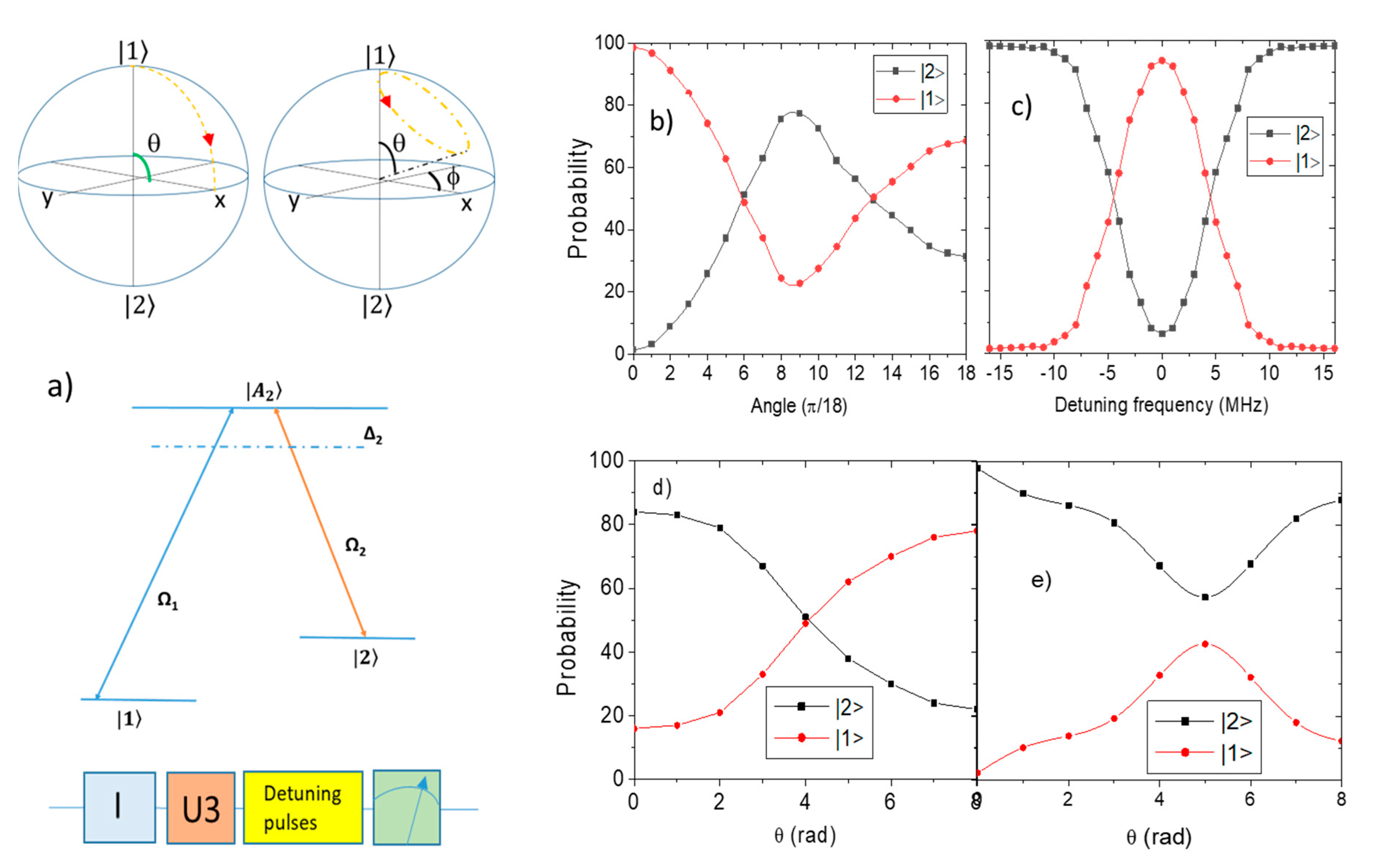
2.1. One Qubit
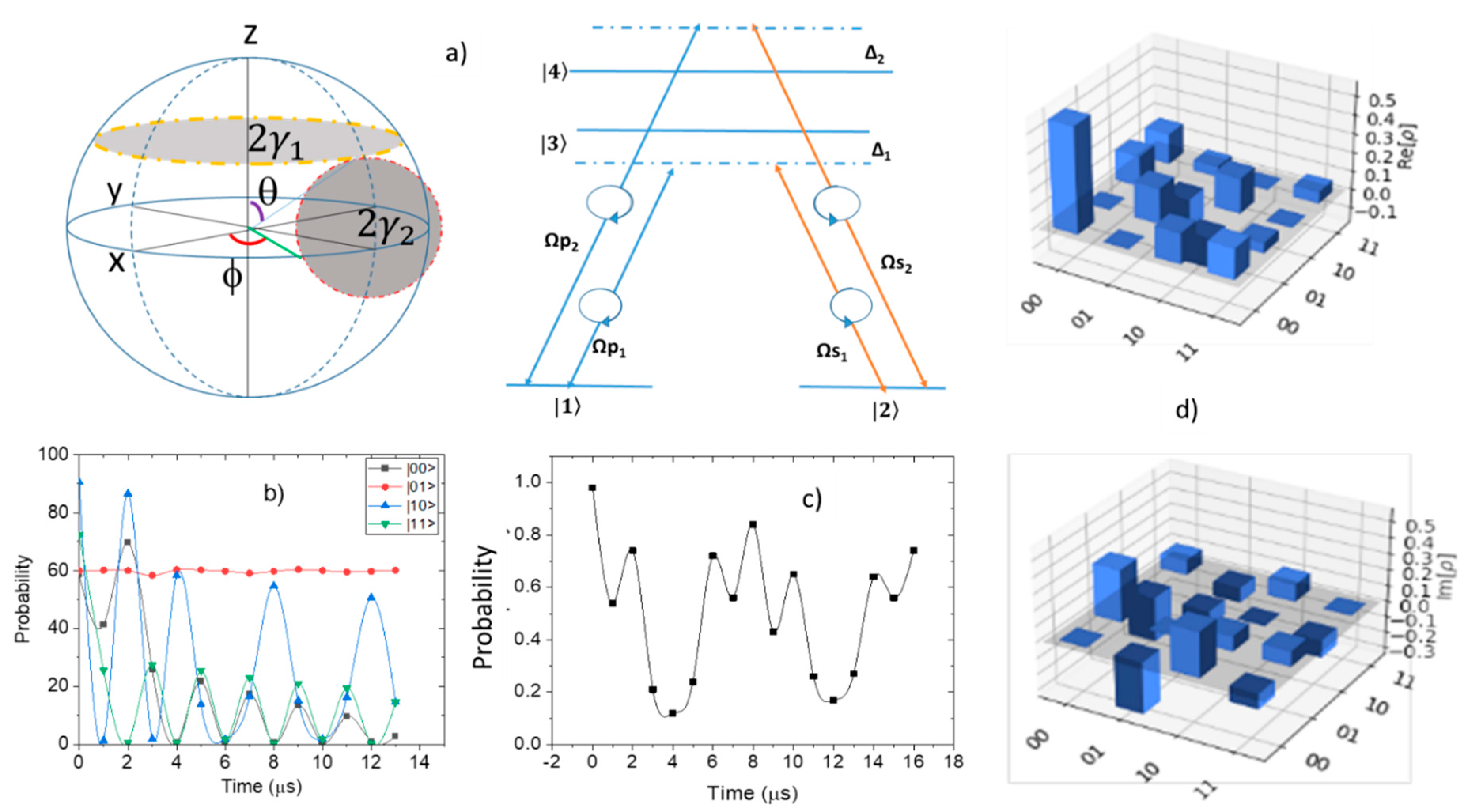
2.2. Two Qubits
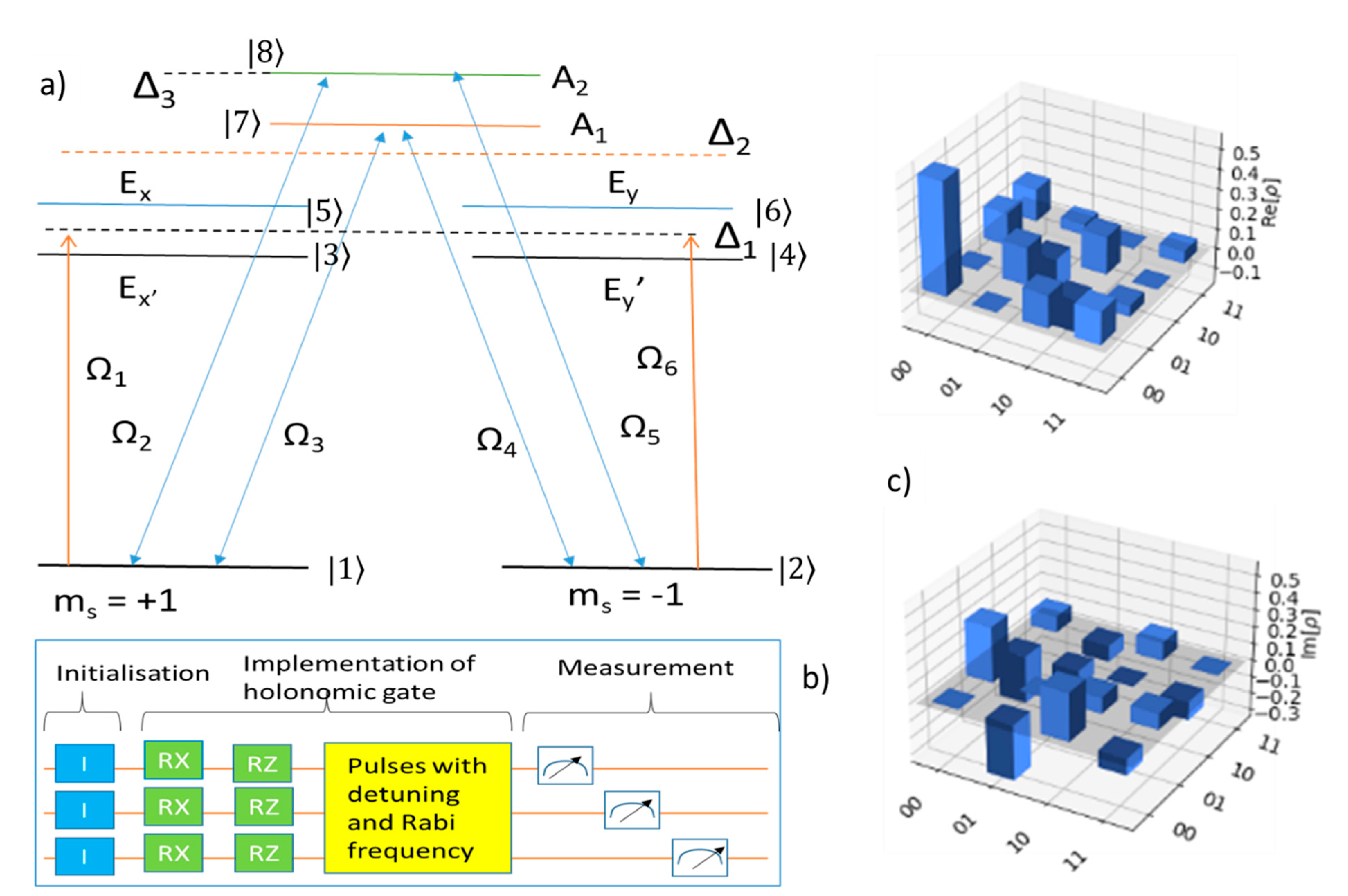
2.3. Three Qubits
3. Discussions
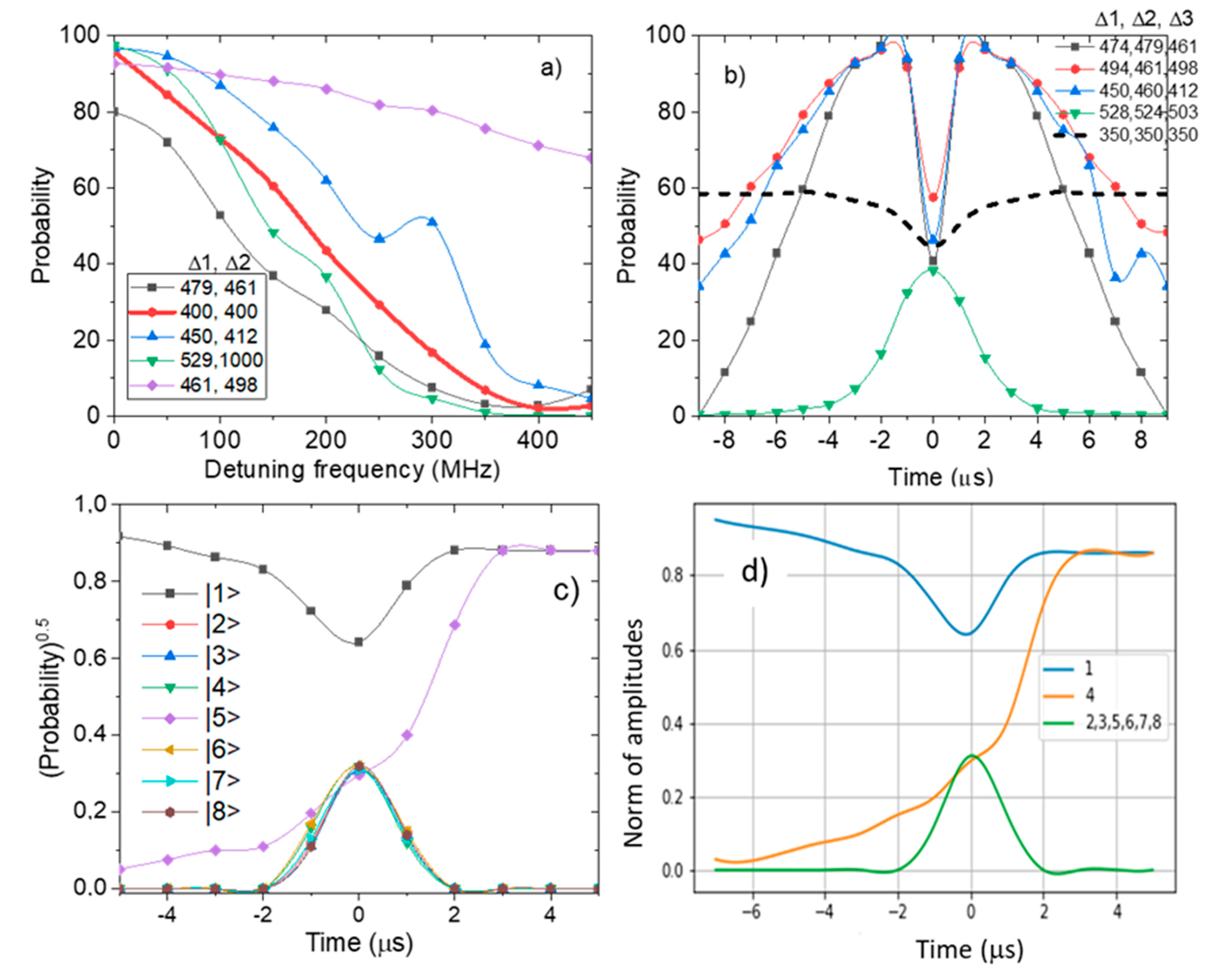
3.1. Dark States
3.2. Fidelity
4. Conclusions
Supplementary Materials
Author Contributions
Funding
Data Availability Statement
Acknowledgments
Conflicts of Interest
References
- Zanardi, P.; Rasetti, M. Holonomic quantum computation. Phys. Lett. A 1999, 264, 94–99. [Google Scholar] [CrossRef] [Green Version]
- Kowarsky, M.A.; Hollenberg, L.C.L.; Martin, A.M. Non-Abelian geometric phase in the diamond nitrogen-vacancy center. Phys. Rev. A 2014, 90, 042116. [Google Scholar] [CrossRef] [Green Version]
- Zhang, J.; Devitt, S.J.; You, J.Q.; Nori, F. Holonomic surface codes for fault-tollerant quantum computation. Phys. Rev. A 2018, 97, 022335. [Google Scholar] [CrossRef] [Green Version]
- Wang, X.G.; Sun, Z.; Wang, Z.D. Operator fidelity susceptibility: An indicator of quantum criticalitym. Phys. Rev. A 2009, 79, 012105. [Google Scholar] [CrossRef] [Green Version]
- Arroyo-Camejo, S.; Lazariev, A.; Hell, S.W.; Balasubramanian, G. Room temperature high-fidelity holonomic single-qubit gate on a solid-state spin. Nat. Commun. 2014, 5, 4870. [Google Scholar] [CrossRef] [Green Version]
- Han, Z.; Dong, Y.; Liu, B.; Yang, X.; Song, S.; Qiu, L.; Li, D.; Chu, J.; Zheng, W.; Xu, J.; et al. Experimental realization of universal time-optimal non-abelian geometric gates. arXiv 2020, arXiv:2004.10364. [Google Scholar]
- Xue, Z.Y.; Zhou, J.; Wang, Z.D. Universal holonomic quantum gates in decoherence-free subspace on superconducting circuits. Phys. Rev. A 2015, 92, 022320. [Google Scholar] [CrossRef] [Green Version]
- Zhao, P.Z.; Xu, G.F.; Tong, D.M. Nonadiabatic holonomic multiqubit controlled gates. Phys. Rev. A 2019, 99, 052309. [Google Scholar] [CrossRef] [Green Version]
- Nagata, K.; Kuramitani, K.; Sekiguchi, Y.; Kosaka, H. Direct evidence for hula twist and single-bond rotation photoproducts. Nat. Commun. 2018, 9, 2510. [Google Scholar]
- Zhou, B.B.; Jerger, P.C.; Shkolnikov, V.O.; Heremans, F.J.; Burkard, G.; Awschalom, D.D. Holonomic quantum control by coherent optical excitation in diamond. Phys. Rev. Lett. 2017, 119, 140503. [Google Scholar] [CrossRef] [Green Version]
- Lu, J.; Zhou, L. Non-Abelian geometrical control of a qubit in an NV center in diamond. EPL 2013, 102, 30006. [Google Scholar] [CrossRef] [Green Version]
- Jelezko, F.; Wrachtrup, J. Processing quantum information in diamond. J. Phys. Condens. Matter 2006, 18, S807–S824. [Google Scholar]
- Dolde, F.; Jakobi, I.; Naydenov, B.; Zhao, N.; Pezzagna, S.; Trautmann, C.; Meijer, J.; Neumann, P.; Jelezko, F.; Wrachtrup, W. Room-temperature entanglement between single defects spins in diamond. Nat. Phys. 2013, 9, 139. [Google Scholar] [CrossRef]
- Wei, H.R.; Long, G.L. Universal photonic quantum gates assisted by ancilla diamond nitrogen-vacancy centers coupled to resonators. Phys. Rev. A 2015, 91, 032324. [Google Scholar] [CrossRef]
- Wu, Y.; Wang, Y.; Qin, X.; Rong, X.; Du, J. A programmable two-qubit solid-state quantum processor under ambient conditions. NPJ Quantum Inf. 2019, 5, 9. [Google Scholar] [CrossRef] [Green Version]
- Rios, J.M. Quantum Manipulation of Nitrogen-Vacancy Centers in Diamond: From Basic Properties to Applications; Harvard University: Cambridge, MA, USA, 2010. [Google Scholar]
- Hopper, D.A.; Shulevitz, H.J.; Bassett, L.C. Spin readout techniques of the nitrogen-vacancy center in diamond. Micromachines 2018, 9, 437. [Google Scholar] [CrossRef] [Green Version]
- Mousolou, V.A. Electric nonadiabatic geometric entangling gates on spin qubits. Phys. Rev. A 2017, 96, 012307. [Google Scholar] [CrossRef] [Green Version]
- Zu, C.; Wang, W.B.; He, L.; Zhang, W.G.; Dai, C.Y.; Wang, F.; Duan, L.M. Experimental realization of universal geometric quantum gates with solid-state spins. Nature 2014, 514, 72. [Google Scholar] [CrossRef] [Green Version]
- Haruyama, M.; Onoda, S.; Higuchi, T.; Kada, W.; Chiba, A.; Hirano, Y.; Teraji, T.; Igarashi, R.; Kawai, S.; Kawarada, H.; et al. Triple nitrogen-vacancy centre fabrication by C5N4Hn ion implantation. Nat. Commun. 2019, 10, 2664. [Google Scholar] [CrossRef] [Green Version]
- Bhattacharyya, S.; Bhattacharyya, S. Demonstrating geometric phase acquisition in multi-path tunnel systems using a near-term quantum computer. J. Appl. Phys. 2021, 130, 034901. [Google Scholar] [CrossRef]
- Xing, T.H.; Wu, X.; Xu, G.F. Nonadiabatic holonomic three-qubit controlled gates realized by one-shot implementation. Phys. Rev. A 2020, 101, 012306. [Google Scholar] [CrossRef]
- Zhao, P.Z.; Li, K.Z.; Xu, G.F.; Tong, D.M. General approach for constructing Hamiltonians for nonadiabatic holonomic quantum computation. Phys. Rev. A 2020, 101, 062306. [Google Scholar] [CrossRef]
- Mazhandu, F.; Mathieson, K.; Coleman, C.; Bhattacharyya, S. Experimental simulation of hybrid quantum systems and entanglement on a quantum computer. Appl. Phys. Lett. 2019, 115, 233501. [Google Scholar] [CrossRef]
- Mahony, D.; Bhattacharyya, S. Evaluation of highly entangled states in asymmetrically coupled three NV centers by quantum simulator. Appl. Phys. Lett. 2021, 118, 204004. [Google Scholar] [CrossRef]
- Xu, K.; Ning, W.; Huang, X.J.; Han, P.R.; Li, H.; Yang, Z.B.; Zheng, D.D.; Fan, H.; Zheng, S.B. Demonstration of a non-Abelian geometric controlled-Not gate in a superconducting circuit. Optica 2021, 8, 972–976. [Google Scholar] [CrossRef]
- Liu, X.; Liu, X.J.; Sinova, J. Spin dynamics in the strong spin-orbit coupling regime—A collective Rabi oscillation. Phys. Rev. B 2011, 84, 035318. [Google Scholar] [CrossRef] [Green Version]
- Doherty, M.W.; Manson, N.B.; Delaney, P.P.; Hollenberg, L.C.L. The negatively charged nitrogen-vacancy centre in diamond: The electronic solution. N. J. Phys. 2011, 13, 025019. [Google Scholar] [CrossRef] [Green Version]
- Roushan, P.; Neill, C.; Chen, Y.; Kolodrubetz, M.; Quintana, C.; Leung, N.; Fang, M.; Barends, R.; Campbell, B.; Chen, Z.; et al. Observation of topological transitions in interacting quantum circuits. Nat. Phys. 2016, 13, 146. [Google Scholar] [CrossRef] [Green Version]
- Wang, D.W.; Song, C.; Feng, W.; Cai, H.; Xu, D.; Deng, H.; Zheng, D.; Zhu, X.; Wang, H.; Zhu, S.; et al. Synthesis of antisymmetric spin exchange interaction and chiral spin clusters in superconducting circuits. Nat. Phys. 2019, 15, 382. [Google Scholar] [CrossRef] [Green Version]
- Bhattacharyya, S.; Mtsuko, D.; Allen, C.; Coleman, C. Effects of rashba-spin-orbit coupling on superconducting boron-doped nanocrystalline diamond films: Evidence of interfacial triplet superconductivity. New J. Phys. 2020, 22, 093039. [Google Scholar] [CrossRef]
- Chen, T.; Shen, P.; Xue, Z.Y. Robust and fast holonomic quantum gates with encoding on superconducting circuits. Phys. Rev. Appl. 2020, 14, 034038. [Google Scholar] [CrossRef]
- Zhang, S.B.; Rui, W.B.; Calzona, A.; Choi, S.J.; Schnyder, A.P.; Trauzettel, B. Topological and holonomic quantum computation based on second-order topological superconductors. Phys. Rev. Res. 2020, 2, 043025. [Google Scholar] [CrossRef]
- Xu, G.F.; Zhao, P.Z.; Sjöqvist, E.; Tong, D.M. Realizing nonadiabatic holonomic quantum computation beyond the three-level setting. Phys. Rev. A 2021, 103, 052605. [Google Scholar] [CrossRef]
- Dong, Y.; Zhang, S.C.; Zheng, Y.; Lin, H.B.; Shan, L.K.; Chen, X.D.; Zhu, W.; Wang, G.Z.; Guo, G.C.; Sun, F.W. Experimental implementation of universal holonomic quantum computation on solid-state spins with optimal control. Phys. Rev. Appl. 2021, 16, 024060. [Google Scholar] [CrossRef]
- Li, S.; Chen, T.; Xue, Z.Y. Fast holonomic quantum computation on superconducting circuits with optimal control. Adv. Quantum Technol. 2020, 3, 2000001. [Google Scholar] [CrossRef] [Green Version]
- Yan, G.A.; Lu, H. The study of security during quantum dense coding in high-dimensions. Int. J. Theo. Phys. 2020, 59, 2223. [Google Scholar] [CrossRef]
- Zhu, X.; Matsuzaki, Y.; Amsűss, R.; Kakuyanagi, K.; Shimo-Oka, T.; Mizuochi, N.; Nemoto, K.; Semba, K.; Munro, W.J.; Saito, S. Observation of dark states in a superconductor diamond quantum hybrid system. Nat. Commun. 2014, 5, 3524. [Google Scholar] [CrossRef] [Green Version]
- Lai, D.G.; Wang, X.; Qin, W.; Hou, B.P.; Nori, F.; Liao, J.Q. Tunable optomechanically induced transparency by controlling the dark-mode effect. Phys. Rev. A 2020, 102, 023707. [Google Scholar] [CrossRef]
- Gu, X.; Kockum, A.F.; Miranowicz, A.; Liu, Y.X.; Nori, F. Microwave photonics with superconducting quantum circuits. Phys. Rep. 2017, 718–719, 1–102. [Google Scholar] [CrossRef]
- Dür, W.; Vidal, G.; Cirac, J.I. Three qubits can be entangled in two inequivalent ways. Phys. Rev. A. 2000, 62, 062314. [Google Scholar] [CrossRef] [Green Version]
- Churochkin, D.; McIntosh, R.; Bhattacharyya, S. Tuning resonant transmission through geometrical configurations of impurity clusters. J. Appl. Phys. 2013, 113, 044305. [Google Scholar] [CrossRef]


Publisher’s Note: MDPI stays neutral with regard to jurisdictional claims in published maps and institutional affiliations. |
© 2022 by the authors. Licensee MDPI, Basel, Switzerland. This article is an open access article distributed under the terms and conditions of the Creative Commons Attribution (CC BY) license (https://creativecommons.org/licenses/by/4.0/).
Share and Cite
Bhattacharyya, S.; Bhattacharyya, S. Demonstration of the Holonomically Controlled Non-Abelian Geometric Phase in a Three-Qubit System of a Nitrogen Vacancy Center. Entropy 2022, 24, 1593. https://doi.org/10.3390/e24111593
Bhattacharyya S, Bhattacharyya S. Demonstration of the Holonomically Controlled Non-Abelian Geometric Phase in a Three-Qubit System of a Nitrogen Vacancy Center. Entropy. 2022; 24(11):1593. https://doi.org/10.3390/e24111593
Chicago/Turabian StyleBhattacharyya, Shaman, and Somnath Bhattacharyya. 2022. "Demonstration of the Holonomically Controlled Non-Abelian Geometric Phase in a Three-Qubit System of a Nitrogen Vacancy Center" Entropy 24, no. 11: 1593. https://doi.org/10.3390/e24111593