

Auxiliary Graph for Attribute Graph Clustering

Abstract
:1. Introduction
- We build an auxiliary graph to reveal the relationships that were missed by the given graph. With the supervising of both auxiliary graph and given graph, the learned representations are improved to be more reliable.
- The optimization by clustering loss based on fusing embeddings from multiple layers facilitates both the discriminativeness and the clustering-awareness of representations.
- Extensive experiments on four popular benchmark datasets are conducted and the results validate the superiority of our method over the state-of-the-art methods.
2. Related Works
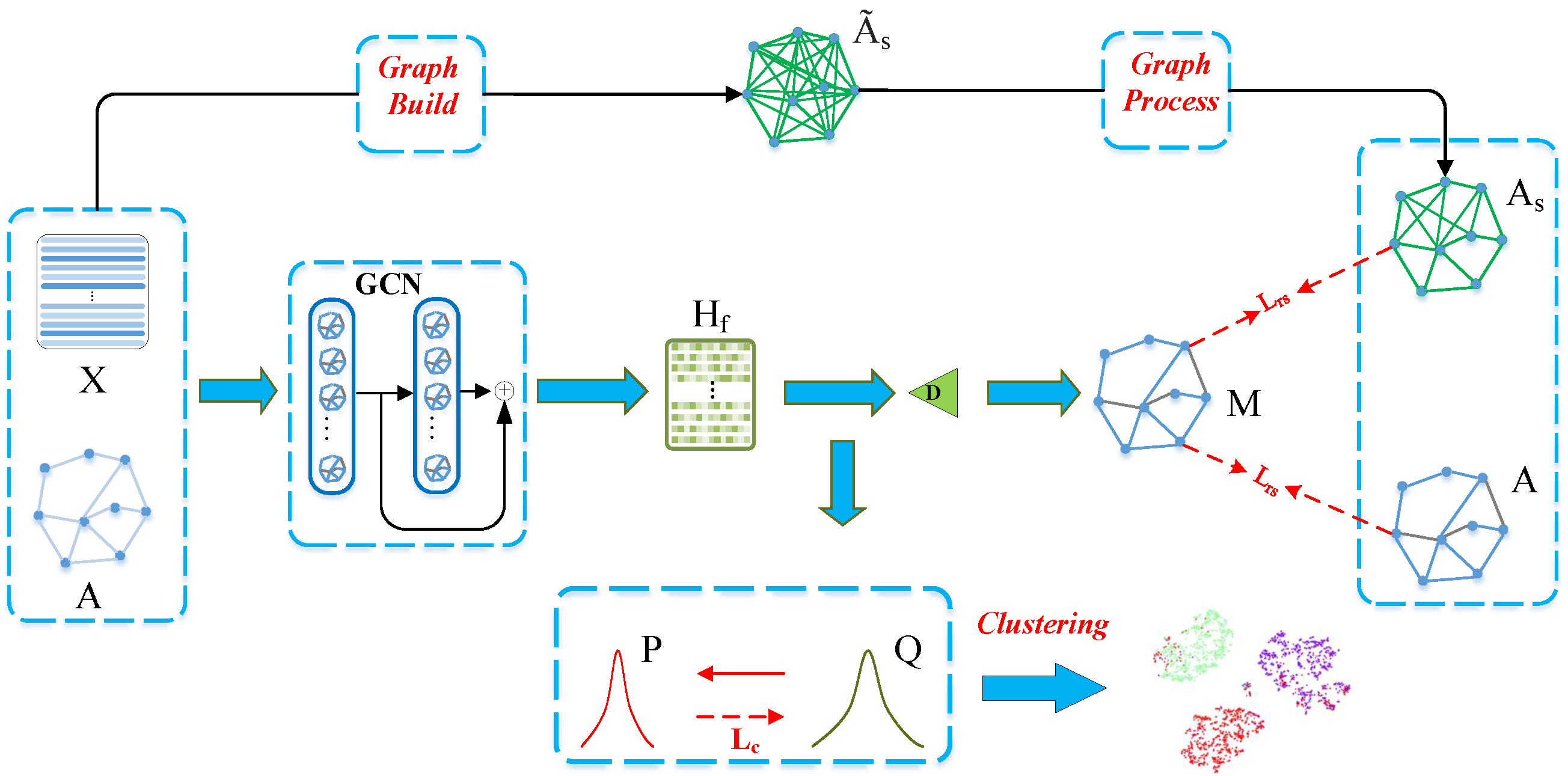
3. Proposed Method
3.1. Problem Definition
3.2. Graph Encoder
3.3. Graph Decoder
3.4. Optimization by Reconstructing Graphs
3.4.1. Optimization by Reconstructing Original Graph
3.4.2. Optimization by Reconstructing Complementary Graph
- Graph Build To make a complement to the given graph, we build a graph based on some similarity metric such as cosine similarity, which can discover the latent relationships between nodes in a global view. The complementary graph is constructed by the following equations:After calculating the similarity between each pair of nodes, we obtain a graph capturing the global relationships.
- Graph Process After graph building, we obtain an initial graph S that unavoidably contains noise. To obtain a relatively clean graph, we need to filter noise. We introduce a simple but effective filtering mechanism.At first, we rank each row of S in descending order by a function. After ranking, . And then, by using a filter mechanism, we only keep relations of top-K highest confidence, and we reduce the rest to 0 to decrease the impact of false relations.
- Minimization of reconstruction loss After the process of filtering, we obtain a more reliable graph . And we implement representation learning by minimizing the loss between M and , which is formulated as:The and are supervisors that are complementary to each other.
3.4.3. The Joint Reconstruction Loss
3.5. Clustering Module
3.6. Joint Optimization
| Algorithm 1 Deep Graph Clustering via Graph Augmentation |
| Require: Attribute matrix X, adjacent matrix A, iteration number , hyperparameter Ensure: Clustering result Y;
|
3.7. Complexity Analysis
4. Experiment
4.1. Datasets
- Citeseer This is a citation dataset. Papers in it are divided into six categories: Agents, Artificial Intelligence, Database, Information Retrieve, Machine Language, HCI. Each edge represents a citation relationship between documents. Each node denotes a paper whose feature is represented by a {0, 1} vector. Each dimension is a keyword from a specific vocabulary.
- Dblp It is a cooperative network. Authors in it are divided into four classes: database, data mining, machine learning, and information retrieval. An edge represents a cooperative relationship between authors. The node features are the elements of a bag-of-words represented by keywords.
- Acm It is a paper network. An edge between nodes represents that these two papers are written by the same author. Papers are divided into three classes: Database, Wireless Communication, and Data Mining. The features are bag-of-words of keywords from corresponding areas.
- Pubmed It is a citation dataset about Diabetes. The publications in it are divided into 3 classes: Diabetes Experimental, Diabetes type1, and Diabetes type2. Each node is represented by a tf-idf vector of keywords.
4.2. Baselines
- K-means A widely used clustering algorithm based on an EM [36] updating strategy.
- AE [10] A classical Deep model for unsupervised learning.
- DEC [11] A deep embedding model based on Auto-Encoder for clustering.
- IDEC [9] A deep model based on DEC with an additional Auto-Encoder module for preserving the local structure of data.
- GAE&VGAE [15] A GCN-based model for unsupervised learning, based on the frameworks of AE&VAE.
- ARGE&ARVGE [16] A GAE (VGAE) based model, with the adversarial training strategy to regularize the distribution of embedding for robust representations.
- DAEGC [19] An attention mechanism based graph clustering model. Instead of being guided by a given graph structure, it learns to aggregate by posing attention scores on each neighbor.
- SDCN [20] A hybrid deep clustering model that integrates embeddings from both Auto-Encoder and GCN module, which is designed for easing the problem of over-smoothness.
- AGCN [34] Based on SDCN, it proposed a method to learn an attention mechanism to fuse the embeddings from different modules reasonably.
- DFCN [21] Based on SDCN, it introduces a cross-modality fusion mechanism to improve the robustness.
4.3. Parameter Settings
4.4. Metrics
4.5. Analysis of Result
- We can observe from these tables that the proposed method outperforms all the compared baseline methods on four benchmark datasets on most metrics. For example, in Dblp, our model outperforms the second-best one by nearly 4 pp (pp: percentage point), 7 pp, 8 pp, 5 pp on ACC, NMI, ARI, and F1 respectively. In Pubmed, compared to the second strongest, our model outperforms it by nearly 2 pp, 3 pp, 3 pp, 2 pp on ACC, NMI, ARI, F1 respectively. There are three reasons for the effectiveness of our model: First, we fuse embeddings from multiple layers to generate discriminative representations; Second, we construct a filtered graph from the original feature space to preserve the global relations of nodes; Last, we develop a joint training strategy to learn representations that can facilitate clustering and preserve both local relations and intrinsic global relations of nodes.
- AE, DEC, and IDEC only use node features for generating embeddings, which leads to a sub-optimal clustering performance compared with GCN-based models. K-means clustering is directly performed in the original feature space, it can be used to measure the quality of features. From k-means, we can observe that the quality of data in Acm is the best.
- In GAE, VGAE, ARGE, and ARVGE, they generate embeddings from a single layer. Compared with them, besides reconstructing intrinsic relationships, our model can fuse multi-scale features to strengthen the discriminativeness for embeddings.
- DAEGC exploited the attention mechanism for aggregating. Although considering the relations between nodes in a wider range, it implements representation learning by the supervision from the given graph structure, which cannot exploit the hidden relations that are missed by the given graph. Compared with it, our model has two advantages: First, we explore relations from a global view. Second, the explored relations come from original space, which can be considered to be more intrinsic.
- SDCN, AGCN, and DFCN are powerful deep clustering models that exploit multi-modality to generate discriminative embeddings. Regardless of alleviating the problem of over-smoothness, these models fail to explore the latent relations of nodes that cannot be observed from the given graph. However, by measuring the similarity between nodes, our model successfully revealed the missing relations from the original feature space and outperforms the mentioned models.
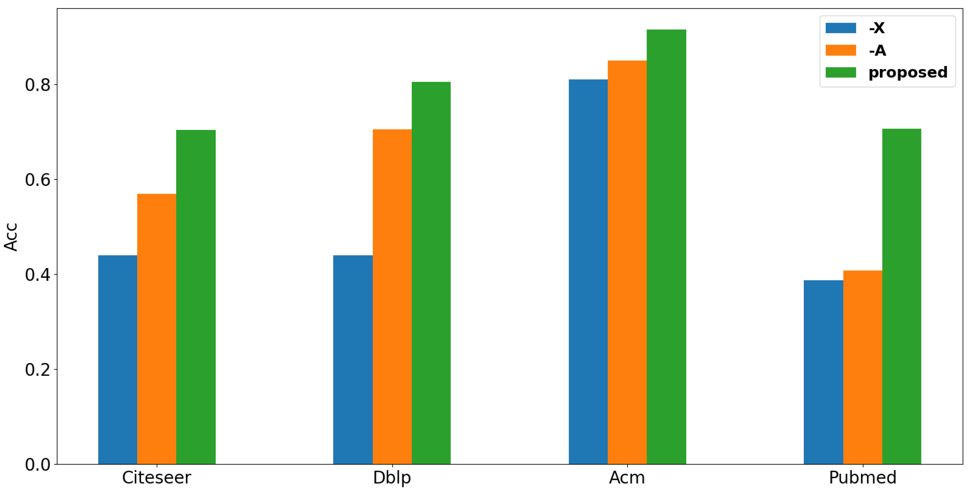
4.6. Ablation Study
4.6.1. The Effectiveness of Each Component
4.6.2. The Effectiveness of Each Layer
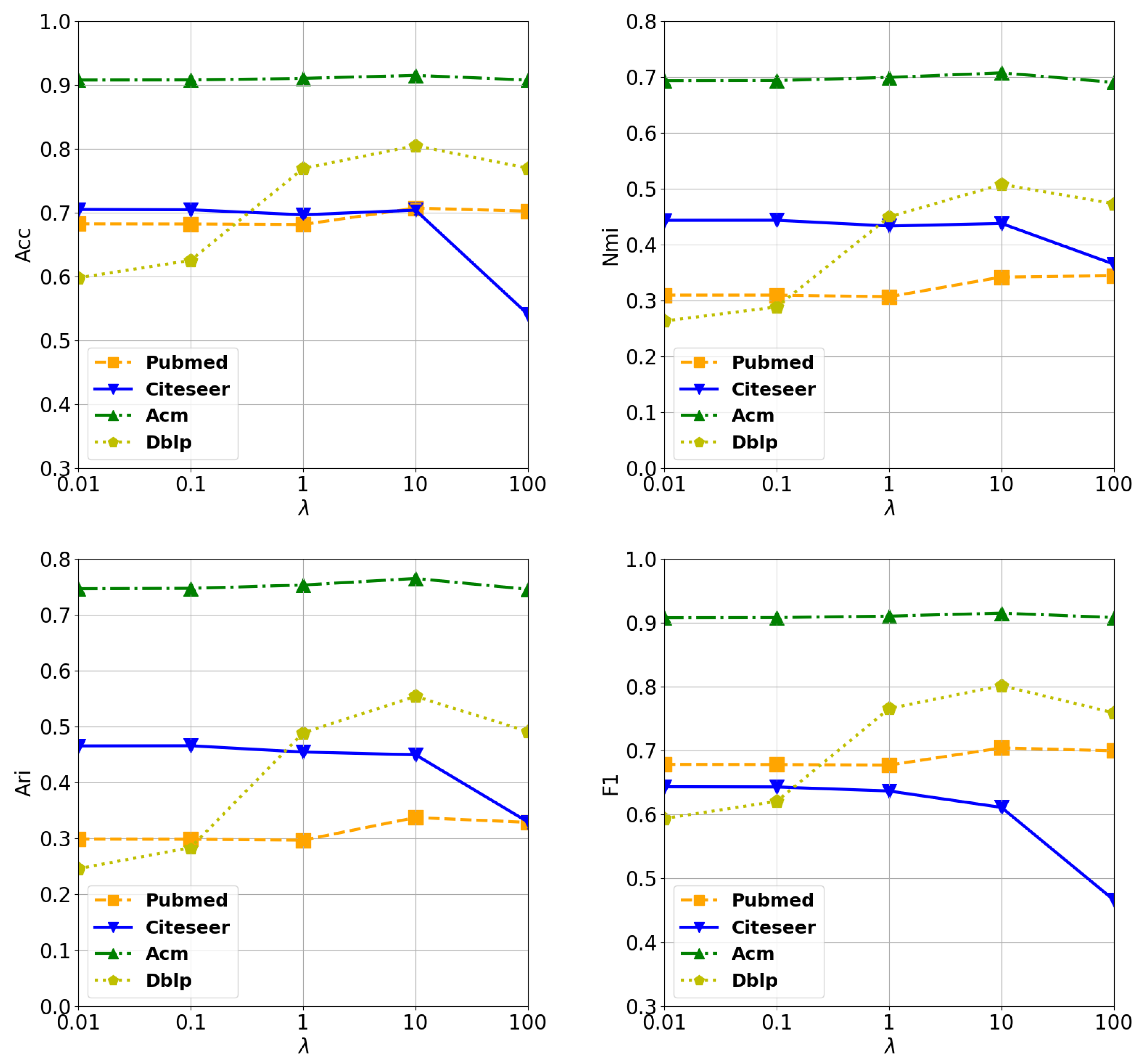
4.7. Analysis of Hyperparameters
4.7.1. Analysis of
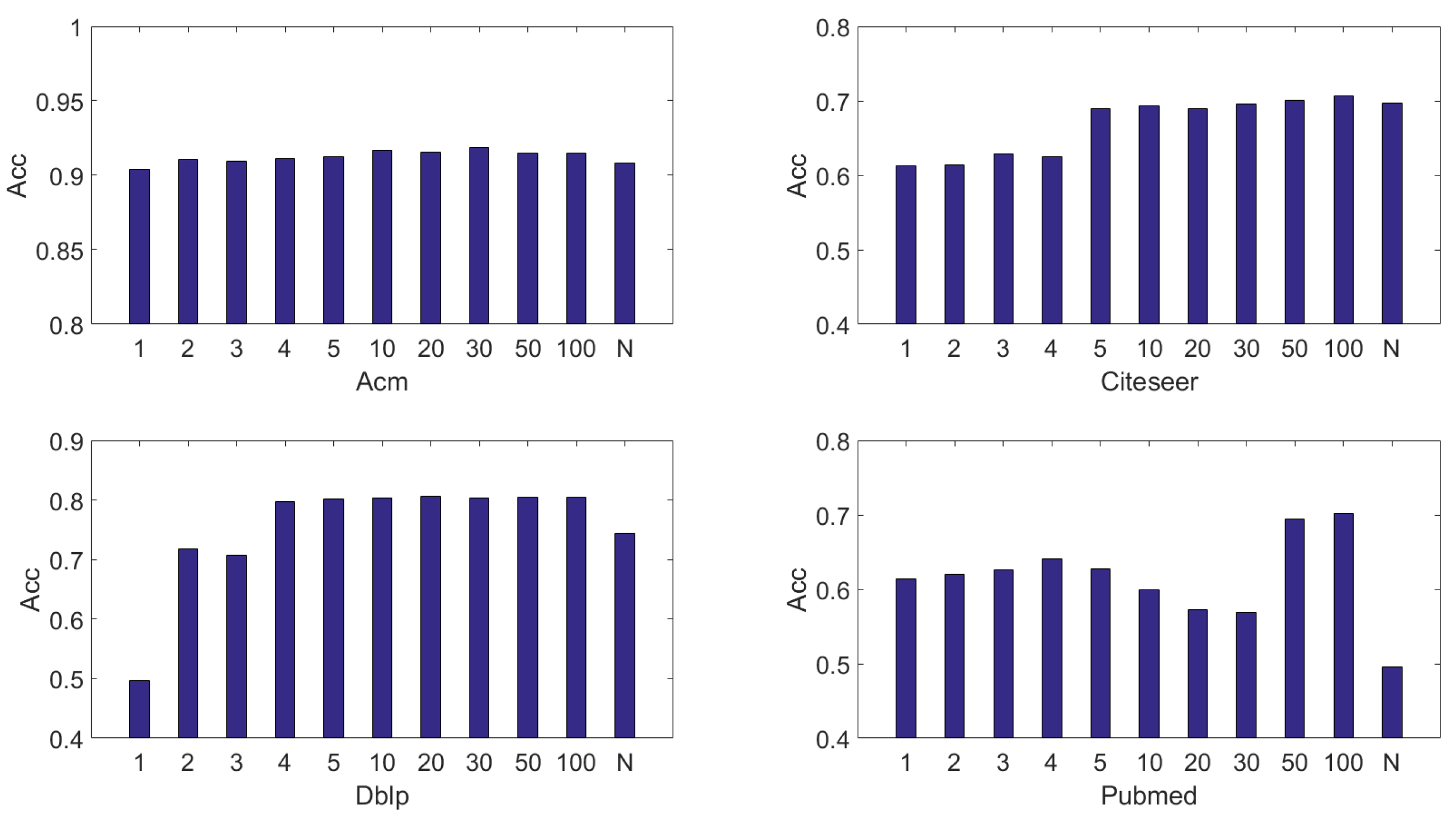
4.7.2. Analysis of K
4.8. Study on the Influence of Graph Structure and Attribute
5. Conclusions
Author Contributions
Funding
Institutional Review Board Statement
Data Availability Statement
Conflicts of Interest
References
- Hastings, M.B. Community detection as an inference problem. Phys. Rev. E 2006, 74, 035102. [Google Scholar] [CrossRef] [PubMed] [Green Version]
- Kipf, T.N.; Welling, M. Semi-Supervised Classification with Graph Convolutional Networks. In Proceedings of the 5th International Conference on Learning Representations (ICLR 2017), Toulon, France, 24–26 April 2017. [Google Scholar]
- Altaf-Ul-Amin, M.; Shinbo, Y.; Mihara, K.; Kurokawa, K.; Kanaya, S. Development and implementation of an algorithm for detection of protein complexes in large interaction networks. BMC Bioinform. 2006, 7, 207. [Google Scholar] [CrossRef] [PubMed]
- Perozzi, B.; Al-Rfou, R.; Skiena, S. DeepWalk: Online learning of social representations. In Proceedings of the 20th ACM SIGKDD International Conference on Knowledge Discovery and Data Mining, New York, NY, USA, 24–27 August 2014; ACM: New York, NY, USA, 2014; pp. 701–710. [Google Scholar]
- Grover, A.; Leskovec, J. node2vec: Scalable Feature Learning for Networks. In Proceedings of the Proceedings of the 22nd ACM SIGKDD International Conference on Knowledge Discovery and Data Mining, San Francisco, CA, USA, 13–17 August 2016; ACM: New York, NY, USA, 2016; pp. 855–864. [Google Scholar]
- Zenil, H.; Kiani, N.A.; Tegnér, J. Algorithmic complexity of motifs clusters superfamilies of networks. In Proceedings of the 2013 IEEE International Conference on Bioinformatics and Biomedicine, Shanghai, China, 18–21 December 2013; Li, G., Kim, S., Hughes, M., McLachlan, G.J., Sun, H., Hu, X., Ressom, H.W., Liu, B., Liebman, M.N., Eds.; IEEE Computer Society: Manhattan, NY, USA, 2013; pp. 74–76. [Google Scholar]
- Zenil, H.; Kiani, N.A.; Marabita, F.; Deng, Y.; Elias, S.; Schmidt, A.; Ball, G.; Tegner, J. An algorithmic information calculus for causal discovery and reprogramming systems. iScience 2019, 19, 1160–1172. [Google Scholar] [CrossRef] [PubMed] [Green Version]
- Zenil, H.; Kiani, N.A.; Zea, A.A.; Tegnér, J. Causal deconvolution by algorithmic generative models. Nat. Mach. Intell. 2019, 1, 58–66. [Google Scholar] [CrossRef] [Green Version]
- Guo, X.; Gao, L.; Liu, X.; Yin, J. Improved Deep Embedded Clustering with Local Structure Preservation. In Proceedings of the Twenty-Sixth International Joint Conference on Artificial Intelligence, Melbourne, Australia, 19–25 August 2017; pp. 1753–1759. [Google Scholar]
- Hinton, G.E.; Salakhutdinov, R.R. Reducing the dimensionality of data with neural networks. Science 2006, 313, 504–507. [Google Scholar] [CrossRef] [PubMed] [Green Version]
- Xie, J.; Girshick, R.B.; Farhadi, A. Unsupervised Deep Embedding for Clustering Analysis. In Proceedings of the 33nd International Conference on Machine Learning, New York City, NY, USA, 20–22 June 2016; Volume 48, pp. 478–487. [Google Scholar]
- Min, E.; Guo, X.; Liu, Q.; Zhang, G.; Cui, J.; Long, J. A Survey of Clustering with Deep Learning: From the Perspective of Network Architecture. IEEE Access 2018, 6, 39501–39514. [Google Scholar] [CrossRef]
- Yang, B.; Fu, X.; Sidiropoulos, N.D.; Hong, M. Towards K-means-friendly Spaces: Simultaneous Deep Learning and Clustering. In Proceedings of the 34th International Conference on Machine Learning (ICML 2017), Sydney, NSW, Australia, 6–11 August 2017; pp. 3861–3870. [Google Scholar]
- Huang, P.; Huang, Y.; Wang, W.; Wang, L. Deep Embedding Network for Clustering. In Proceedings of the 22nd International Conference on Pattern Recognition (ICPR 2014), Stockholm, Sweden, 24–28 August 2014; IEEE Computer Society: Manhattan, NY, USA, 2014; pp. 1532–1537. [Google Scholar]
- Kipf, T.N.; Welling, M. Variational Graph Auto-Encoders. arXiv 2016, arXiv:1611.07308. [Google Scholar]
- Pan, S.; Hu, R.; Long, G.; Jiang, J.; Yao, L.; Zhang, C. Adversarially Regularized Graph Autoencoder for Graph Embedding. In Proceedings of the Twenty-Seventh International Joint Conference on Artificial Intelligence (IJCAI 2018), Stockholm, Sweden, 13–19 July 2018; pp. 2609–2615. [Google Scholar]
- Wang, C.; Pan, S.; Long, G.; Zhu, X.; Jiang, J. MGAE: Marginalized Graph Autoencoder for Graph Clustering. In Proceedings of the 2017 ACM on Conference on Information and Knowledge Management, Singapore, 6–10 November 2017; ACM: New York, NY, USA, 2017; pp. 889–898. [Google Scholar]
- Velickovic, P.; Cucurull, G.; Casanova, A.; Romero, A.; Liò, P.; Bengio, Y. Graph Attention Networks. arXiv 2017, arXiv:1710.10903. [Google Scholar]
- Wang, C.; Pan, S.; Hu, R.; Long, G.; Jiang, J.; Zhang, C. Attributed Graph Clustering: A Deep Attentional Embedding Approach. In Proceedings of the Twenty-Eighth International Joint Conference on Artificial Intelligence, Macao, China, 10–16 August 2019; pp. 3670–3676. [Google Scholar]
- Bo, D.; Wang, X.; Shi, C.; Zhu, M.; Lu, E.; Cui, P. Structural Deep Clustering Network. In Proceedings of the WWW ’20: The Web Conference 2020, Taipei, Taiwan, 20–24 April 2020; ACM: New York, NY, USA, 2020; pp. 1400–1410. [Google Scholar]
- Tu, W.; Zhou, S.; Liu, X.; Guo, X.; Cai, Z.; Zhu, E.; Cheng, J. Deep Fusion Clustering Network. In Proceedings of the Thirty-Fifth AAAI Conference on Artificial Intelligence, AAAI 2021, Thirty-Third Conference on Innovative Applications of Artificial Intelligence, IAAI 2021, The Eleventh Symposium on Educational Advances in Artificial Intelligence (EAAI 2021), Virtual Event, 2–9 February 2021; AAAI Press: Palo Alto, CA, USA, 2021; pp. 9978–9987. [Google Scholar]
- Ji, P.; Zhang, T.; Li, H.; Salzmann, M.; Reid, I.D. Deep Subspace Clustering Networks. In Proceedings of the Advances in Neural Information Processing Systems 30: Annual Conference on Neural Information Processing Systems 2017, Long Beach, CA, USA, 4–9 December 2017; pp. 24–33. [Google Scholar]
- Li, F.; Qiao, H.; Zhang, B. Discriminatively boosted image clustering with fully convolutional auto-encoders. Pattern Recognit. 2018, 83, 161–173. [Google Scholar] [CrossRef] [Green Version]
- Dizaji, K.G.; Herandi, A.; Deng, C.; Cai, W.; Huang, H. Deep Clustering via Joint Convolutional Autoencoder Embedding and Relative Entropy Minimization. In Proceedings of the IEEE International Conference on Computer Vision (ICCV 2017), Venice, Italy, 22–29 October 2017; IEEE Computer Society: Manhattan, NY, USA, 2017; pp. 5747–5756. [Google Scholar] [CrossRef] [Green Version]
- Jiang, Z.; Zheng, Y.; Tan, H.; Tang, B.; Zhou, H. Variational Deep Embedding: An Unsupervised and Generative Approach to Clustering. In Proceedings of the Twenty-Sixth International Joint Conference on Artificial Intelligence, IJCAI 2017, Melbourne, Australia, 19–25 August 2017; Sierra, C., Ed.; 2017; pp. 1965–1972. [Google Scholar] [CrossRef] [Green Version]
- Yang, J.; Parikh, D.; Batra, D. Joint Unsupervised Learning of Deep Representations and Image Clusters. In Proceedings of the 2016 IEEE Conference on Computer Vision and Pattern Recognition (CVPR 2016), Las Vegas, NV, USA, 27–30 June 2016; IEEE Computer Society: Manhattan, NY, USA, 2016; pp. 5147–5156. [Google Scholar] [CrossRef]
- Hsu, C.; Lin, C. CNN-Based Joint Clustering and Representation Learning with Feature Drift Compensation for Large-Scale Image Data. IEEE Trans. Multim. 2018, 20, 421–429. [Google Scholar] [CrossRef] [Green Version]
- Wang, Z.; Chang, S.; Zhou, J.; Wang, M.; Huang, T.S. Learning A Task-Specific Deep Architecture For Clustering. In Proceedings of the 2016 SIAM International Conference on Data Mining, Miami, FL, USA, 5–7 May 2016; Venkatasubramanian, S.C., Meira, W., Eds.; 2016; pp. 369–377. [Google Scholar] [CrossRef] [Green Version]
- Peng, X.; Xiao, S.; Feng, J.; Yau, W.; Yi, Z. Deep Subspace Clustering with Sparsity Prior. In Proceedings of the Twenty-Fifth International Joint Conference on Artificial Intelligence (IJCAI 2016), New York, NY, USA, 9–15 July 2016; Kambhampati, S., Ed.; IJCAI/AAAI Press: Palo Alto, CA, USA, 2016; pp. 1925–1931. [Google Scholar]
- Chen, D.; Lv, J.; Zhang, Y. Unsupervised Multi-Manifold Clustering by Learning Deep Representation. In Proceedings of the The Workshops of the The Thirty-First AAAI Conference on Artificial Intelligence, San Francisco, CA, USA, 4–9 February 2017; AAAI Technical Report. AAAI Press: Palo Alto, CA, USA, 2017; Volume WS-17. [Google Scholar]
- Doersch, C. Tutorial on Variational Autoencoders. arXiv 2016, arXiv:1606.05908. [Google Scholar]
- Li, X.; Zhang, H.; Zhang, R. Embedding Graph Auto-Encoder with Joint Clustering via Adjacency Sharing. arXiv 2020, arXiv:2002.08643. [Google Scholar]
- Zhang, X.; Liu, H.; Li, Q.; Wu, X. Attributed Graph Clustering via Adaptive Graph Convolution. In Proceedings of the Twenty-Eighth International Joint Conference on Artificial Intelligence, Macao, China, 10–16 August 2019; pp. 4327–4333. [Google Scholar]
- Peng, Z.; Liu, H.; Jia, Y.; Hou, J. Attention-driven Graph Clustering Network. In Proceedings of the MM ’21: ACM Multimedia Conference, Virtual Event, China, 20–24 October 2021; ACM: New York, NY, USA, 2021; pp. 935–943. [Google Scholar]
- Pan, S.; Hu, R.; Fung, S.f.; Long, G.; Jiang, J.; Zhang, C. Learning graph embedding with adversarial training methods. IEEE Trans. Cybern. 2019, 50, 2475–2487. [Google Scholar] [CrossRef]
- Dempster, A.P.; Laird, N.M.; Rubin, D.B. Maximum Likelihood from Incomplete Data Via the EM Algorithm. J. R. Stat. Soc. Ser. B (Methodol.) 1977, 39, 1–22. [Google Scholar]


| Notations | Meaning |
|---|---|
| Feature matrix | |
| Adjacent matrix | |
| Identity matrix | |
| Filtered similarity matrix | |
| Adjacent matrix with self-loop | |
| Normalized adjacent matrix | |
| Constructed similarity matrix | |
| Degree matrix | |
| Output of graph encoder | |
| Reconstructed matrix | |
| Constructed similarity matrix | |
| Soft assignment distribution | |
| Target distribution |
| Dataset | Nodes | Dimension | Clusters | Edges | Degree |
|---|---|---|---|---|---|
| Citeseer | 3327 | 3703 | 6 | 4732 | 99 |
| Dblp | 4058 | 334 | 4 | 7056 | 45 |
| Acm | 3025 | 1870 | 3 | 26,256 | 90 |
| Pubmed | 19,717 | 500 | 3 | 44,325 | 142 |
| Method | ACC | NMI | ARI | F1 |
|---|---|---|---|---|
| k-means | 55.06 | 29.21 | 24.56 | 53.03 |
| AE | 53.93 | 27.56 | 26.03 | 50.53 |
| DEC | 60.96 | 33.36 | 33.20 | 57.13 |
| IDEC | 63.16 | 36.54 | 36.75 | 60.37 |
| GAE | 60.55 | 36.34 | 35.50 | 56.24 |
| VGAE | 51.41 | 28.96 | 24.88 | 49.48 |
| ARGE | 54.40 | 26.10 | 24.50 | 52.90 |
| ARVGE | 57.30 | 35.00 | 34.10 | 54.60 |
| DAEGC | 64.54 | 36.41 | 37.78 | 62.20 |
| SDCN | 65.96 | 38.71 | 40.157 | 63.62 |
| AGCN | 68.79 | 41.54 | 43.79 | 62.37 |
| DFCN | 69.50 | 43.90 | 45.50 | 64.30 |
| AGAGC | 70.46 | 44.36 | 46.56 | 64.28 |
| Method | ACC | NMI | ARI | F1 |
|---|---|---|---|---|
| k-means | 59.83 | 31.05 | 28.1 | 58.88 |
| AE | 63.07 | 26.32 | 23.86 | 64.01 |
| DEC | 60.154 | 22.44 | 19.55 | 61.49 |
| IDEC | 60.70 | 23.67 | 20.58 | 62.41 |
| GAE | 62.09 | 23.84 | 20.62 | 61.37 |
| VGAE | 68.48 | 30.61 | 30.155 | 67.68 |
| ARGE | 65.26 | 24.8 | 24.35 | 65.69 |
| ARVGE | 64.25 | 23.88 | 22.82 | 64.51 |
| DAEGC | 68.73 | 28.26 | 29.84 | 68.23 |
| SDCN | 64.20 | 22.87 | 22.30 | 65.01 |
| AGCN | 63.61 | 23.31 | 22.36 | 64.19 |
| DFCN | 68.89 | 31.43 | 30.64 | 68.10 |
| AGAGC | 70.77 | 34.33 | 33.81 | 70.46 |
| Method | ACC | NMI | ARI | F1 |
|---|---|---|---|---|
| k-means | 38.35 | 10.99 | 6.68 | 32.10 |
| AE | 38.62 | 14.03 | 7.41 | 31.72 |
| DEC | 61.46 | 27.53 | 25.25 | 61.82 |
| IDEC | 55.92 | 24.56 | 18.37 | 56.82 |
| GAE | 53.42 | 29.29 | 16.83 | 54.9 |
| VGAE | 53.06 | 28.87 | 16.65 | 54.34 |
| ARGE | 64.44 | 30.21 | 26.21 | 64.32 |
| ARVGE | 61.94 | 25.63 | 23.91 | 60.57 |
| DAEGC | 62.05 | 32.49 | 21.03 | 61.75 |
| SDCN | 68.05 | 39.50 | 39.15 | 67.71 |
| AGCN | 73.26 | 39.68 | 42.49 | 72.80 |
| DFCN | 76.00 | 43.70 | 47.00 | 75.70 |
| AGAGC | 80.50 | 50.77 | 55.41 | 80.16 |
| Method | ACC | NMI | ARI | F1 |
|---|---|---|---|---|
| k-means | 68.17 | 33.40 | 31.29 | 68.42 |
| AE | 78.55 | 44.53 | 46.98 | 78.69 |
| DEC | 72.52 | 43.50 | 43.48 | 70.60 |
| IDEC | 78.33 | 50.83 | 51.52 | 76.44 |
| GAE | 89.06 | 64.69 | 70.47 | 89.05 |
| VGAE | 76.78 | 43.33 | 41.14 | 76.96 |
| ARGE | 83.06 | 49.31 | 55.77 | 84.81 |
| ARVGE | 83.65 | 52.11 | 57.08 | 81.40 |
| DAEGC | 86.94 | 56.18 | 59.35 | 87.07 |
| SDCN | 90.45 | 68.31 | 73.91 | 90.42 |
| AGCN | 90.59 | 68.38 | 74.20 | 90.58 |
| DFCN | 90.90 | 69.40 | 74.90 | 90.80 |
| AGAGC | 91.50 | 70.74 | 76.49 | 91.51 |
| Dataset | Remove | ACC | NMI | ARI | F1 |
|---|---|---|---|---|---|
| Citeseer | w/o S | 65.29 | 40.26 | 40.15 | 58.81 |
| w/o C | 57.24 | 36.82 | 31.76 | 50.26 | |
| w/o A | 70.35 | 43.70 | 45.12 | 62.09 | |
| Proposed | 70.46 | 44.36 | 46.56 | 64.28 | |
| Acm | w/o S | 90.54 | 68.50 | 74.04 | 90.58 |
| w/o C | 89.87 | 67.12 | 72.51 | 59.87 | |
| w/o A | 88.96 | 65.65 | 69.95 | 89.07 | |
| Proposed | 91.60 | 70.74 | 76.49 | 91.51 | |
| Dblp | w/o S | 59.03 | 25.55 | 23.64 | 58.58 |
| w/o C | 80.11 | 50.31 | 55.11 | 79.68 | |
| w/o A | 77.64 | 49.05 | 49.37 | 77.70 | |
| Proposed | 80.50 | 50.77 | 55.41 | 80.16 | |
| Pubmed | w/o S | 62.15 | 24.78 | 21.40 | 62.14 |
| w/o C | 39.95 | - | - | 19.04 | |
| w/o A | 55.60 | 18.20 | 14.53 | 54.31 | |
| Proposed | 70.77 | 34.33 | 33.81 | 70.46 |
| Dataset | Layer | ACC | NMI | ARI | F1 |
|---|---|---|---|---|---|
| Citeseer | 67.76 | 41.80 | 42.29 | 63.73 | |
| 67.95 | 41.56 | 40.93 | 59.52 | ||
| 70.46 | 44.36 | 46.56 | 64.28 | ||
| Dblp | 78.11 | 47.81 | 51.30 | 77.36 | |
| 80.08 | 50.15 | 55.11 | 79.62 | ||
| 80.50 | 50.77 | 55.41 | 80.16 | ||
| Acm | 89.60 | 66.98 | 71.65 | 89.67 | |
| 90.62 | 69.19 | 74.41 | 90.63 | ||
| 91.50 | 70.74 | 76.49 | 91.51 | ||
| Pubmed | 63.73 | 26.03 | 24.37 | 64.98 | |
| 62.91 | 21.34 | 20.63 | 63.31 | ||
| 70.77 | 34.33 | 33.81 | 70.46 |
Publisher’s Note: MDPI stays neutral with regard to jurisdictional claims in published maps and institutional affiliations. |
© 2022 by the authors. Licensee MDPI, Basel, Switzerland. This article is an open access article distributed under the terms and conditions of the Creative Commons Attribution (CC BY) license (https://creativecommons.org/licenses/by/4.0/).
Share and Cite
Li, W.; Wang, S.; Guo, X.; Zhou, Z.; Zhu, E. Auxiliary Graph for Attribute Graph Clustering. Entropy 2022, 24, 1409. https://doi.org/10.3390/e24101409
Li W, Wang S, Guo X, Zhou Z, Zhu E. Auxiliary Graph for Attribute Graph Clustering. Entropy. 2022; 24(10):1409. https://doi.org/10.3390/e24101409
Chicago/Turabian StyleLi, Wang, Siwei Wang, Xifeng Guo, Zhenyu Zhou, and En Zhu. 2022. "Auxiliary Graph for Attribute Graph Clustering" Entropy 24, no. 10: 1409. https://doi.org/10.3390/e24101409