
Intelligent Fault Diagnosis of Rolling-Element Bearings Using a Self-Adaptive Hierarchical Multiscale Fuzzy Entropy


Abstract
:1. Introduction
- (1)
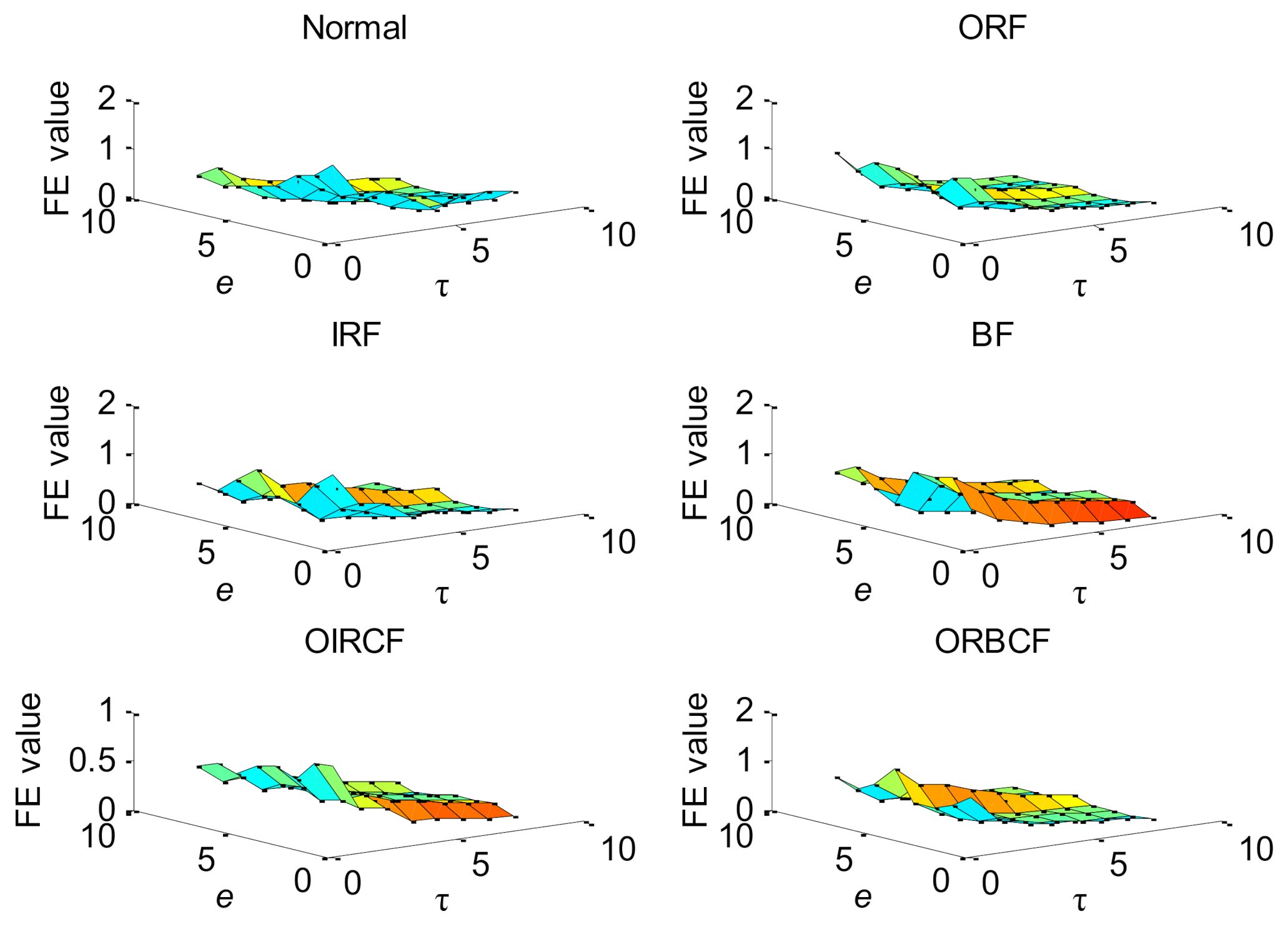
- A novel signal complexity metric method named hierarchical multiscale fuzzy entropy (HMFE) is proposed via integrating hierarchic analysis into multiscale fuzzy entropy, which can effectively obtain more comprehensive and richer bearing fault feature information.
- (2)
- The important parameters of HMFE are selected automatically by using the bird swarm algorithm (BSA) method, which can effectively avoid the disadvantages of manual selecting of the important parameters of the existing entropy.
- (3)
- An intelligent bearing fault diagnosis method based on HMFE is presented, which can improve the identification accuracy of different health conditions of rolling-element bearings.
- (4)
- Two experimental cases and comparative analysis are conducted to verify the effectiveness and superiority of the proposed method.
2. Self-Adaptive Hierarchical Multiscale Fuzzy Entropy
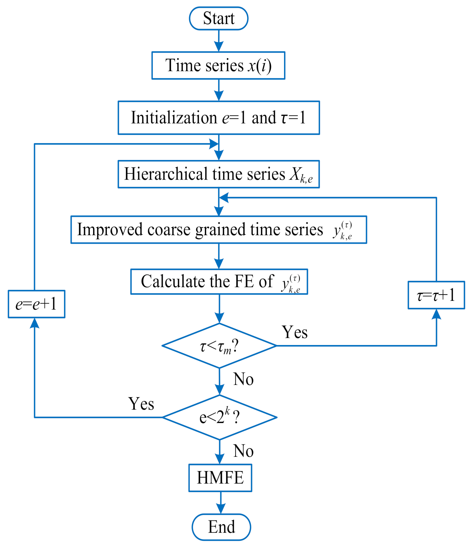
2.1. HMFE
- (1)
- Firstly, the average and difference operator are respectively defined as follows:where n denotes the positive integer, represents the length of the two operators, and and represent the low-frequency and high-frequency components of the original time series in the first layer decomposition, respectively.
- (2)
- Then, to implement the hierarchical analysis of a time series, when j = 0 or 1, the matrix form of the k-th layer operator is expressed as:
- (3)
- To obtain the hierarchical components of each layer in the process of hierarchical decomposition, here we define a one-dimensional vector as and an integral value as , where represents the average or difference operator at the p-th layer. Accordingly, the hierarchical component of the e-th node in the k-th layer can be expressed as:where x represents the given time series.
- (4)
- Next, the improved coarse-grained time series of each hierarchical component at the scale factor can be calculated bywhere N represents the length of the given time series x.
- (5)
- According to the definition of fuzzy entropy, calculate the fuzzy entropy of each improved coarse-grained series , so the final hierarchical multiscale fuzzy entropy can be obtained by the following:where represents the fuzzy entropy operation, m is the embedded dimension, k is the decomposition level, e represents the hierarchical node, denotes the scale factor, is the similarity tolerance controlling the width of membership function, and SD is the standard deviation of the original time series. In Figure 1, represents the predefined largest scale factor.
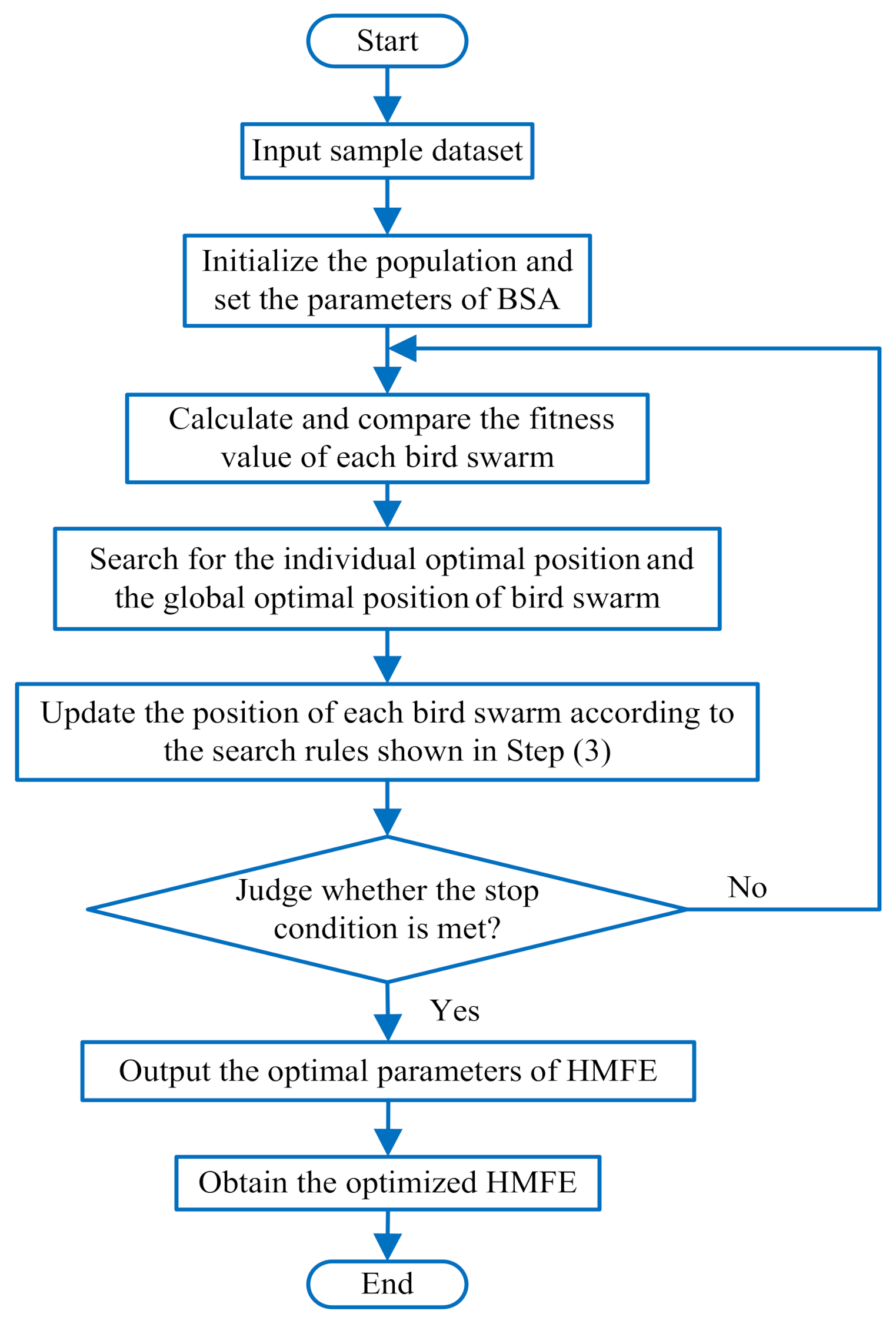
2.2. Adaptive Parameter Selection of HMFE
- (1)
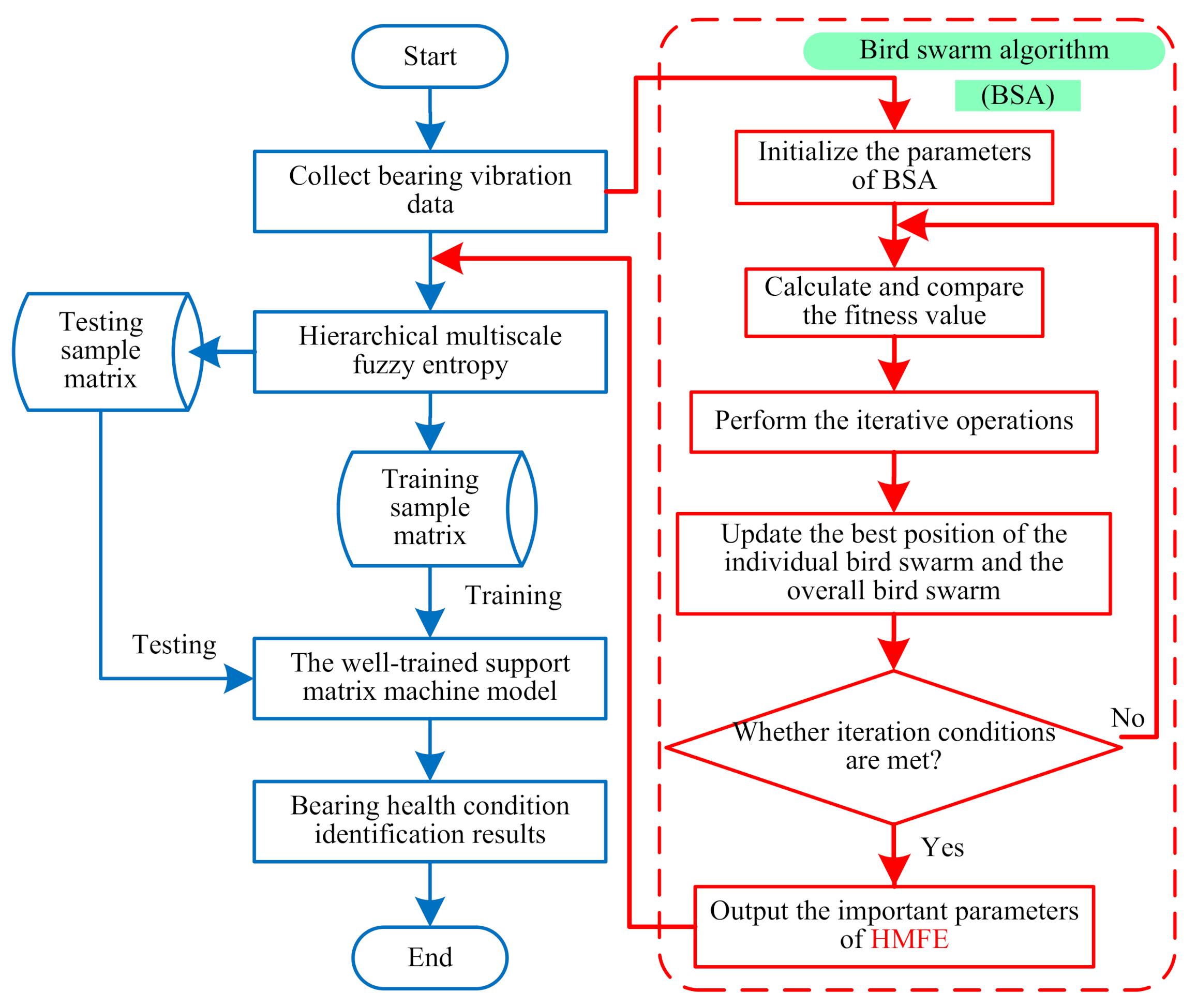
- Initialize the population and set the BSA parameters. When the number of iterations t = 0, set the bird swarm size to N = 30 and the maximum iteration number to M = 50, initialize the flight frequency FQ, foraging frequency P, and several constants (i.e., C, S, FL, a1 and a2).
- (2)
- Calculate and compare the fitness value. According to the fitness function shown in Equation (7), the fitness value of bird swarm is calculated and compared to determine the optimal position of the individual and whole bird swarm.where xi is the number of misclassified samples, xc is the number of samples correctly classified, and fitness(i) is the current fitness value of the i-th bird. When fitness(i) achieves the maximum value, pi,j is the corresponding optimal position of the individual bird swarm, and gj is the corresponding optimal position of the whole bird swarm.
- (3)
- The iterative operation is performed repeatedly, and the position update formula is determined by judging whether the operation t% × FQ has a remainder. Specific rules are summarized as follows:
- (4)
- Update the position of each bird swarm according to the rules in step (3). If the individual of the current bird swarm is better than the individual of the previous bird swarm, the current individual bird swarm is regarded as the optimal position. Otherwise, the previous individual bird swarm is retained as the optimal position to continue the update of bird swarm.
- (5)
- Judge whether the stop condition is met. If the maximum number of iterations or the minimum error rate is reached, the whole optimization process will be stopped, and the optimal position of bird swarm (i.e., the optimal combination parameters of HMFE) will be outputted. Otherwise, the iteration process will continue to be conducted until the stop condition is satisfied.
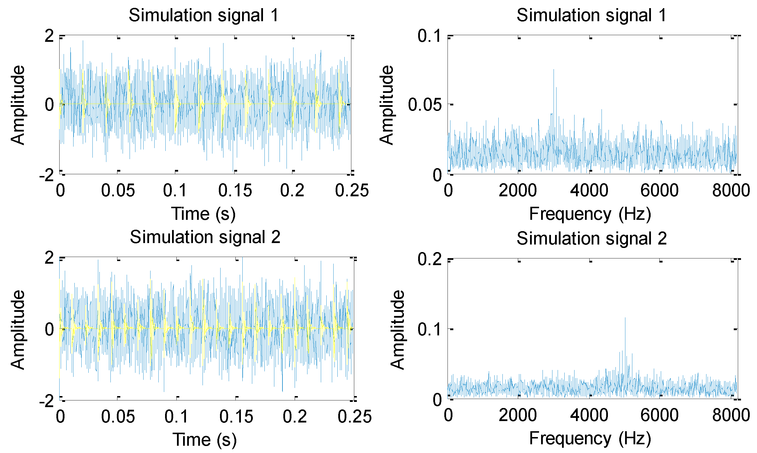
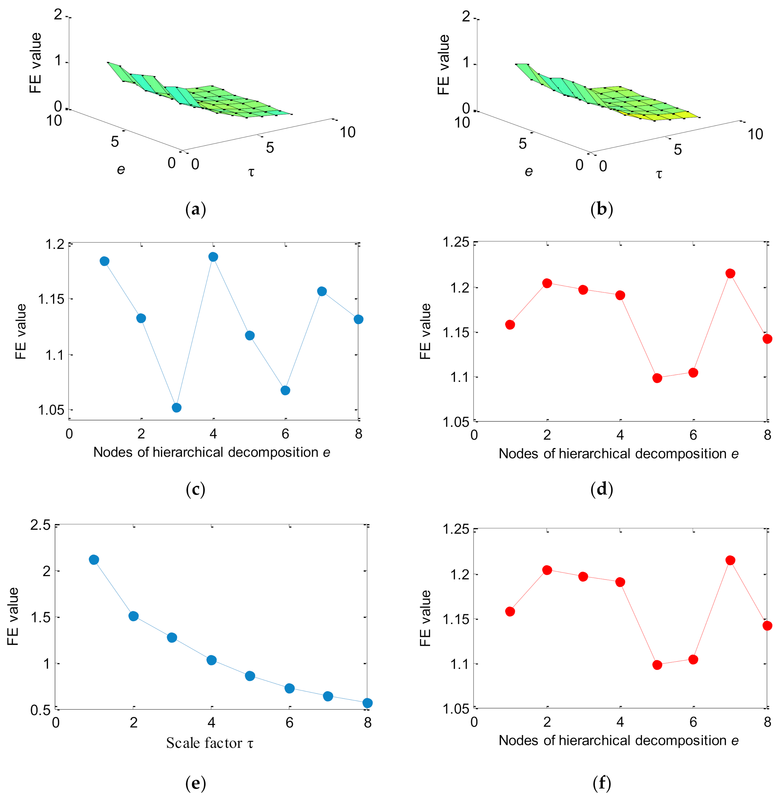
2.3. Comparison Analysis Using Simulation Signal
3. Support Matrix Machine
4. Proposed Method
5. Experimental Verification
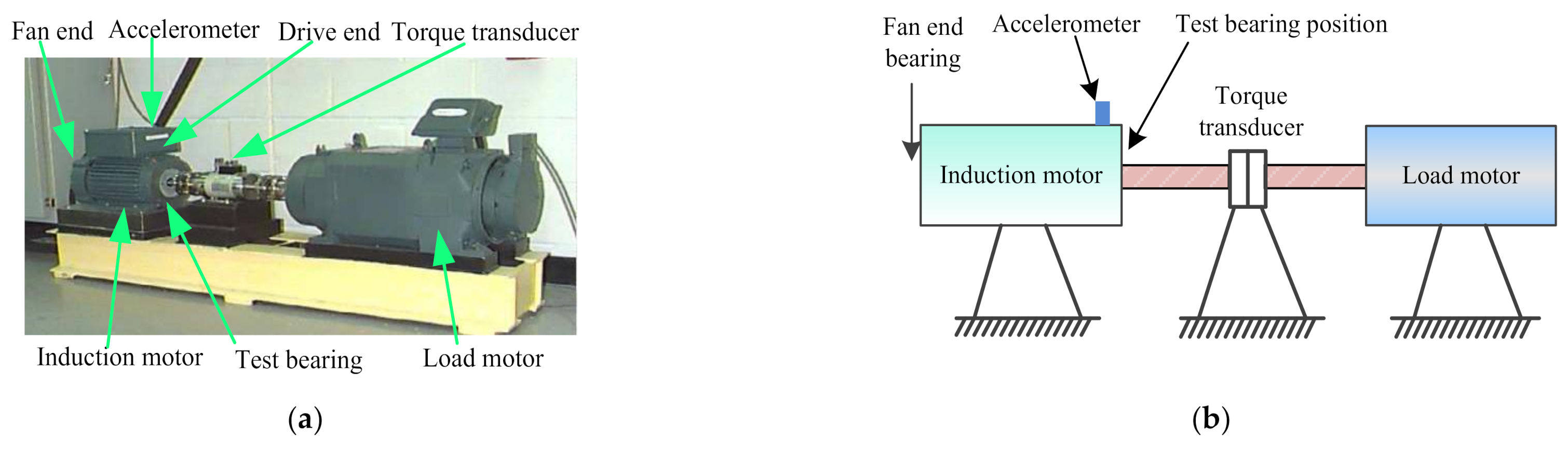
5.1. Case 1: Bearing Benchmark Data from CWRU
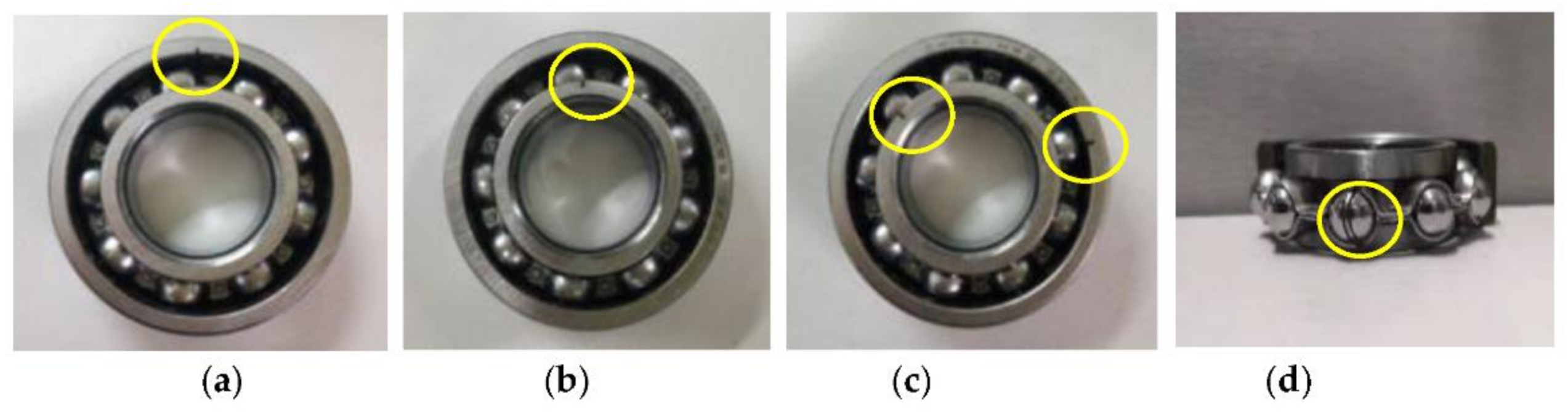
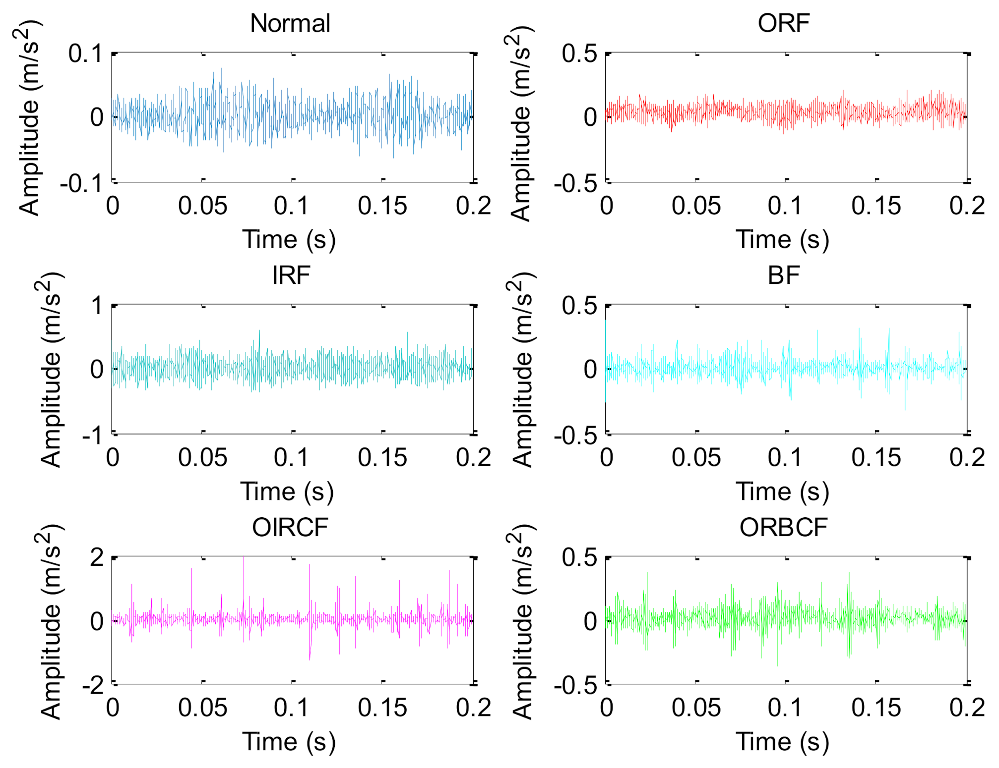
5.2. Case 2: Bearing Vibration Data from Laboratory
5.3. Further Discussion
- (1)
- In the proposed method, the key parameters of HMFE are determined by the bird swarm algorithm (BSA) method, which is helpful for bearing fault feature extraction. We all know that some other advanced optimizer (e.g., Grey wolf optimization (GWO), Whale optimization algorithm (WOA), Grasshopper optimization algorithm (GOA)) can also be introduced to automatically determine the key parameters of HMFE. Therefore, in our future work, the parameter selection problem of HMFE will continue to be studied by adopting other advanced optimizers instead of the BSA method.
- (2)
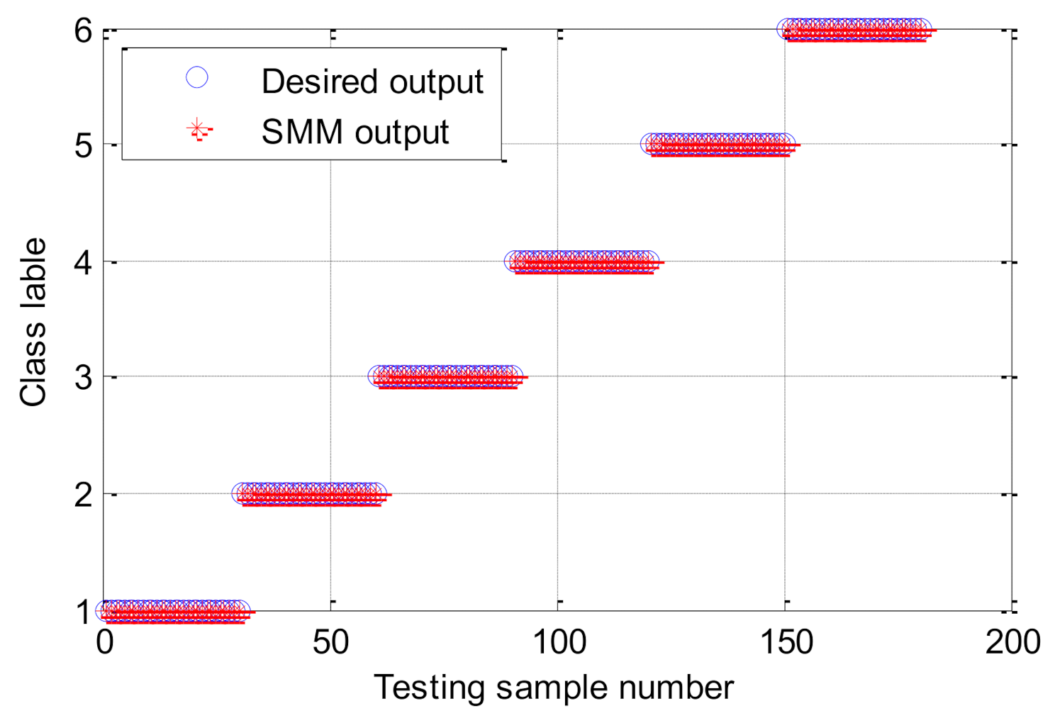
- In the final step of the proposed method, although the support matrix machine (SMM) is employed to achieve the automatic identification of fault patterns of rolling-element bearing and obtain a good diagnosis result, there are many other advanced classification models in the previously reported literature, including the improved versions (e.g., the non-parallel least squares support matrix machine [42], nonlinear kernel support matrix machine) of SMM and deep learning models (e.g., convolutional neural network [43], deep regularized variational autoencoder [44], deep belief network [45], and other deep learning methods [46]). Hence, in our future work, SMM of the proposed method will be replaced by these advanced classification models to automatically obtain the identification results of bearing fault patterns.
- (3)
- The proposed method is proven to be effective for identifying the bearing health condition at constant speed, but it is unknown for bearing fault identification under variable speed. Hence, the proposed method will be extended to solve the problem of bearing fault identification under variable speed, which is regarded as our future focus. Besides this, in our future work, other faults (e.g., gear, rotor, and blade) of rotating machinery will also be diagnosed by applying the proposed method.
- (4)
- In this paper, the proposed HMFE is only applied for single-channel sensor data analysis of rolling-element bearings. For bearing vibration data analysis of multi-channel sensors, with the help of the idea of multichannel data processing used in the existing multivariate multiscale entropy, a new multichannel data processing method named multivariate hierarchical multiscale fuzzy entropy (MHMFE) will be designed to solve the problem of multivariate fault diagnosis in our future work.
- (5)
- Due to the addition of the parameter optimization algorithm, the biggest limitation of the proposed method lies in the large calculation time. Therefore, to solve this issue and improve the computational efficiency of the proposed method, in our future work, some sensitive indicators (e.g., Chebychev distance and Mahalanobis distance) can be used to instead of the complex optimizer to automatically select the key parameters of HMFE. Besides, in the running of the algorithm, graphic processing units (GPU) can be adopted instead of the central processing unit (CPU) to accelerate the calculation process of the proposed method.
6. Conclusions
- (1)
- A new signal complexity metric method named hierarchical multiscale fuzzy entropy is developed by integrating the hierarchical decomposition into multiscale fuzzy entropy, which is aimed at improving fault feature extraction performance.
- (2)
- An effective parameter optimizer called bird swarm algorithm is introduced to automatically choose several important parameters of hierarchical multiscale fuzzy entropy, which can avoid the dependence of parameter selection of the existing entropy on specialist experience.
- (3)
- The effectiveness of the proposed method in the identification of bearing fault types and fault severity is verified by experimental and contrastive analysis. The experimental results show that compared with some existing representative multiscale entropies or hierarchical entropies, the proposed method can achieve broader and richer fault feature information and its identification accuracy has been greatly improved, which indicates that the proposed method has a certain competitiveness in bearing health condition identification. This study provides a new perspective for intelligent fault diagnosis for rolling-element bearings.
Author Contributions
Funding
Institutional Review Board Statement
Informed Consent Statement
Data Availability Statement
Acknowledgments
Conflicts of Interest
References
- Yan, X.; Liu, Y.; Jia, M. Multiscale cascading deep belief network for fault identification of rotating machinery under various working conditions. Knowl. Based Syst. 2020, 193, 105484. [Google Scholar] [CrossRef]
- Wang, X.; Si, S.; Wei, Y.; Li, Y. The optimized multi-scale permutation entropy and its application in compound fault diagnosis of rotating machinery. Entropy 2019, 21, 170. [Google Scholar] [CrossRef] [Green Version]
- Ye, M.; Yan, X.; Jia, M. Rolling bearing fault diagnosis based on VMD-MPE and PSO-SVM. Entropy 2021, 23, 762. [Google Scholar] [CrossRef] [PubMed]
- Zhang, F.; Sun, W.; Wang, H.; Xu, T. Fault diagnosis of a wind turbine gearbox based on improved variational mode algorithm and information entropy. Entropy 2021, 23, 794. [Google Scholar] [CrossRef] [PubMed]
- Chen, C.; Tian, H.; Wu, D.; Pan, Q.; Wang, H.; Liu, X. A fault diagnosis method for satellite flywheel bearings based on 3D correlation dimension clustering technology. IEEE Access 2018, 6, 78483–78492. [Google Scholar] [CrossRef]
- Hong, H.; Liang, M. Fault severity assessment for rolling element bearings using the Lempel–Ziv complexity and continuous wavelet transform. J. Sound Vib. 2009, 320, 452–468. [Google Scholar] [CrossRef]
- Hao, R.; Peng, Z.; Feng, Z.; Chu, F. Application of support vector machine based on pattern spectrum entropy in fault diagnostics of rolling element bearings. Meas. Sci. Technol. 2011, 22, 45708. [Google Scholar] [CrossRef]
- Yan, R.; Gao, R.X. Approximate entropy as a diagnostic tool for machine health monitoring. Mech. Syst. Signal Process. 2007, 21, 824–839. [Google Scholar] [CrossRef]
- Han, M.; Pan, J. A fault diagnosis method combined with LMD, sample entropy and energy ratio for roller bearings. Measurement 2015, 76, 7–19. [Google Scholar] [CrossRef]
- Bandt, C.; Pompe, B. Permutation entropy: A natural complexity measure for time series. Phys. Rev. Lett. 2002, 88, 174102. [Google Scholar] [CrossRef] [PubMed]
- Yan, X.; Liu, Y.; Jia, M. A fault diagnosis approach for rolling bearing integrated SGMD, IMSDE and multiclass relevance vector machine. Sensors 2020, 20, 4352. [Google Scholar] [CrossRef]
- Azami, H.; Escudero, J. Amplitude-and fluctuation-based dispersion entropy. Entropy 2018, 20, 210. [Google Scholar] [CrossRef] [PubMed] [Green Version]
- Deng, W.; Zhang, S.; Zhao, H.; Yang, X. A novel fault diagnosis method based on integrating empirical wavelet transform and fuzzy entropy for motor bearing. IEEE Access 2018, 6, 35042–35056. [Google Scholar] [CrossRef]
- Ma, J.; Li, Z.; Li, C.; Zhan, L.; Zhang, G.Z. Rolling bearing fault diagnosis based on refined composite multi-scale approximate entropy and optimized probabilistic neural network. Entropy 2021, 23, 259. [Google Scholar] [CrossRef] [PubMed]
- Wu, S.D.; Wu, C.W.; Lin, S.G.; Wang, C.C.; Lee, K.Y. Time series analysis using composite multiscale entropy. Entropy 2013, 15, 1069–1084. [Google Scholar] [CrossRef] [Green Version]
- Tang, G.; Wang, X.; He, Y. A novel method of fault diagnosis for rolling bearing based on dual tree complex wavelet packet transform and improved multiscale permutation entropy. Math. Probl. Eng. 2016, 2016, 5432648. [Google Scholar] [CrossRef] [Green Version]
- Zheng, J.; Cheng, J.; Yang, Y. Multiscale permutation entropy based rolling bearing fault diagnosis. Shock Vib. 2014, 2014, 1–8. [Google Scholar] [CrossRef]
- Han, M.; Wu, Y.; Wang, Y.; Liu, W. Roller bearing fault diagnosis based on LMD and multi-scale symbolic dynamic information entropy. J. Mech. Sci. Technol. 2021, 35, 1993–2005. [Google Scholar] [CrossRef]
- Yan, X.; Jia, M. Intelligent fault diagnosis of rotating machinery using improved multiscale dispersion entropy and mRMR feature selection. Knowl. Based Syst. 2019, 163, 450–471. [Google Scholar] [CrossRef]
- Li, Y.; Miao, B.; Zhang, W.; Chen, P.; Liu, J.; Jiang, X. Refined composite multiscale fuzzy entropy: Localized defect detection of rolling element bearing. J. Mech. Sci. Technol. 2019, 33, 109–120. [Google Scholar] [CrossRef]
- Han, B.; Wang, S.; Zhu, Q.; Yang, X.; Li, Y. Intelligent fault diagnosis of rotating machinery using hierarchical Lempel-Ziv complexity. Appl. Sci. 2020, 10, 4221. [Google Scholar] [CrossRef]
- Yan, X.; Liu, Y.; Ding, P.; Jia, M. Fault diagnosis of rolling-element bearing using multiscale pattern gradient spectrum entropy coupled with Laplacian score. Complexity 2020, 2020, 1–29. [Google Scholar] [CrossRef] [Green Version]
- Gao, Y.; Villecco, F.; Li, M.; Song, W. Multi-scale permutation entropy based on improved LMD and HMM for rolling bearing diagnosis. Entropy 2017, 19, 176. [Google Scholar] [CrossRef] [Green Version]
- Wu, S.D.; Wu, P.H.; Wu, C.W.; Ding, J.J.; Wang, C.C. Bearing fault diagnosis based on multiscale permutation entropy and support vector machine. Entropy 2012, 14, 1343–1356. [Google Scholar] [CrossRef] [Green Version]
- Gan, X.; Lu, H.; Yang, G. Fault diagnosis method for rolling bearings based on composite multiscale fluctuation dispersion entropy. Entropy 2019, 21, 290. [Google Scholar] [CrossRef] [Green Version]
- Zheng, J.; Pan, H.; Yang, S.; Cheng, J. Generalized composite multiscale permutation entropy and Laplacian score based rolling bearing fault diagnosis. Mech. Syst. Signal Process. 2018, 99, 229–243. [Google Scholar] [CrossRef]
- Wang, Z.; Yao, L.; Cai, Y. Rolling bearing fault diagnosis using generalized refined composite multiscale sample entropy and optimized support vector machine. Measurement 2020, 156, 107574. [Google Scholar] [CrossRef]
- Tang, G.; Pang, B.; He, Y.; Tian, T. Gearbox fault diagnosis based on hierarchical instantaneous energy density dispersion entropy and dynamic time warping. Entropy 2019, 21, 593. [Google Scholar] [CrossRef] [Green Version]
- Li, Y.; Xu, M.; Zhao, H.; Huang, W. Hierarchical fuzzy entropy and improved support vector machine based binary tree approach for rolling bearing fault diagnosis. Mech. Mach. Theory 2016, 98, 114–132. [Google Scholar] [CrossRef]
- Li, Y.; Xu, M.; Wang, R.; Huang, W. A fault diagnosis scheme for rolling bearing based on local mean decomposition and improved multiscale fuzzy entropy. J. Sound Vib. 2016, 360, 277–299. [Google Scholar] [CrossRef]
- Meng, X.; Gao, X.; Lu, L.; Liu, Y.; Zhang, H. A new bio-inspired optimisation algorithm: Bird swarm algorithm. J. Exp. Theor. Artif. In. 2016, 28, 1–15. [Google Scholar] [CrossRef]
- Yan, X.; Jia, M.; Xiang, L. Compound fault diagnosis of rotating machinery based on OVMD and a 1.5-dimension envelope spectrum. Meas. Sci. Technol. 2016, 27, 075002. [Google Scholar] [CrossRef]
- Haidong, S.; Hongkai, J.; Xingqiu, L.; Shuaipeng, W. Intelligent fault diagnosis of rolling bearing using deep wavelet auto-encoder with extreme learning machine. Knowl. Based Syst. 2018, 140, 1–14. [Google Scholar] [CrossRef]
- Yan, X.; Liu, Y.; Xu, Y.; Jia, M. Multichannel fault diagnosis of wind turbine driving system using multivariate singular spectrum decomposition and improved Kolmogorov complexity. Renew. Energ. 2021, 170, 724–748. [Google Scholar] [CrossRef]
- Luo, L.; Xie, Y.; Zhang, Z.; Li, W.J. Support matrix machines. In Proceedings of the 32nd International Conference on Machine Learning, Lille, France, 6–11 July 2015. [Google Scholar]
- Lancaster, P.; Tismenetsky, M. The Theory of Matrices with Application; Academic Press: Cambridge, MA, USA, 1985. [Google Scholar]
- Tan, H.; Cheng, B.; Feng, J.; Feng, G.; Wang, W.; Zhang, Y.J. Low-n-rank tensor recovery based on multi-linear augmented Lagrange multiplier method. Neurocomputing 2013, 119, 144–152. [Google Scholar] [CrossRef]
- Ho, K.; Newman, S. State of the art electrical discharge machining (EDM). Int. J. Mach. Tool. Manuf. 2003, 43, 1287–1300. [Google Scholar] [CrossRef]
- Yan, X.; Jia, M. A novel optimized SVM classification algorithm with multi-domain feature and its application to fault diagnosis of rolling bearing. Neurocomputing 2018, 313, 47–64. [Google Scholar] [CrossRef]
- Luo, S.; Yang, W.; Luo, Y. Fault Diagnosis of a rolling bearing based on adaptive sparest narrow-band decomposition and refined composite multiscale dispersion entropy. Entropy 2020, 22, 375. [Google Scholar]
- Zhu, K.; Song, X.; Xue, D. A roller bearing fault diagnosis method based on hierarchical entropy and support vector machine with particle swarm optimization algorithm. Measurement 2014, 47, 669–675. [Google Scholar] [CrossRef]
- Li, X.; Yang, Y.; Pan, H.; Cheng, J. Non-parallel least squares support matrix machine for rolling bearing fault diagnosis. Mech. Mach. Theory 2020, 145, 103676. [Google Scholar] [CrossRef]
- Xie, C.; Liu, Y.; Zeng, W.; Lu, X. An improved method for single image super-resolution based on deep learning. Signal Image Video Process. 2019, 13, 557–565. [Google Scholar] [CrossRef]
- Yan, X.; She, D.; Xu, Y.; Jia, M. Deep regularized variational autoencoder for intelligent fault diagnosis of rotor-bearing system within entire life-cycle process. Knowl. Based Syst. 2021, 226, 107142. [Google Scholar] [CrossRef]
- Liu, F.; Liu, B.; Sun, C.; Liu, M.; Wang, X. Deep belief network-based approaches for link prediction in signed social networks. Entropy 2015, 17, 2140–2169. [Google Scholar] [CrossRef] [Green Version]
- Yu, Y.; Liu, Y.; Chen, J.; Jiang, D.; Zhuang, Z.; Wu, X. Detection method for bolted connection looseness at small angles of timber structures based on deep learning. Sensors 2021, 21, 3106. [Google Scholar] [CrossRef]


| Methods | Euclidean Distance | Calculation Time (s) |
|---|---|---|
| HMFE | 0.3421 | 5.167 |
| HFE | 0.2048 | 2.163 |
| MFE | 0.0613 | 9.768 |
| Bearing Type | Roller Diameter (mm) | Pitch Diameter (mm) | Number of the Roller | Contact Angle (°) |
|---|---|---|---|---|
| SKF6205-2RS | 7.94 | 39.04 | 9 | 0 |
| Bearing Health Conditions | Abbreviation | Fault Size (inches) | Number of Training Samples | Number of Testing Samples | Class Label |
|---|---|---|---|---|---|
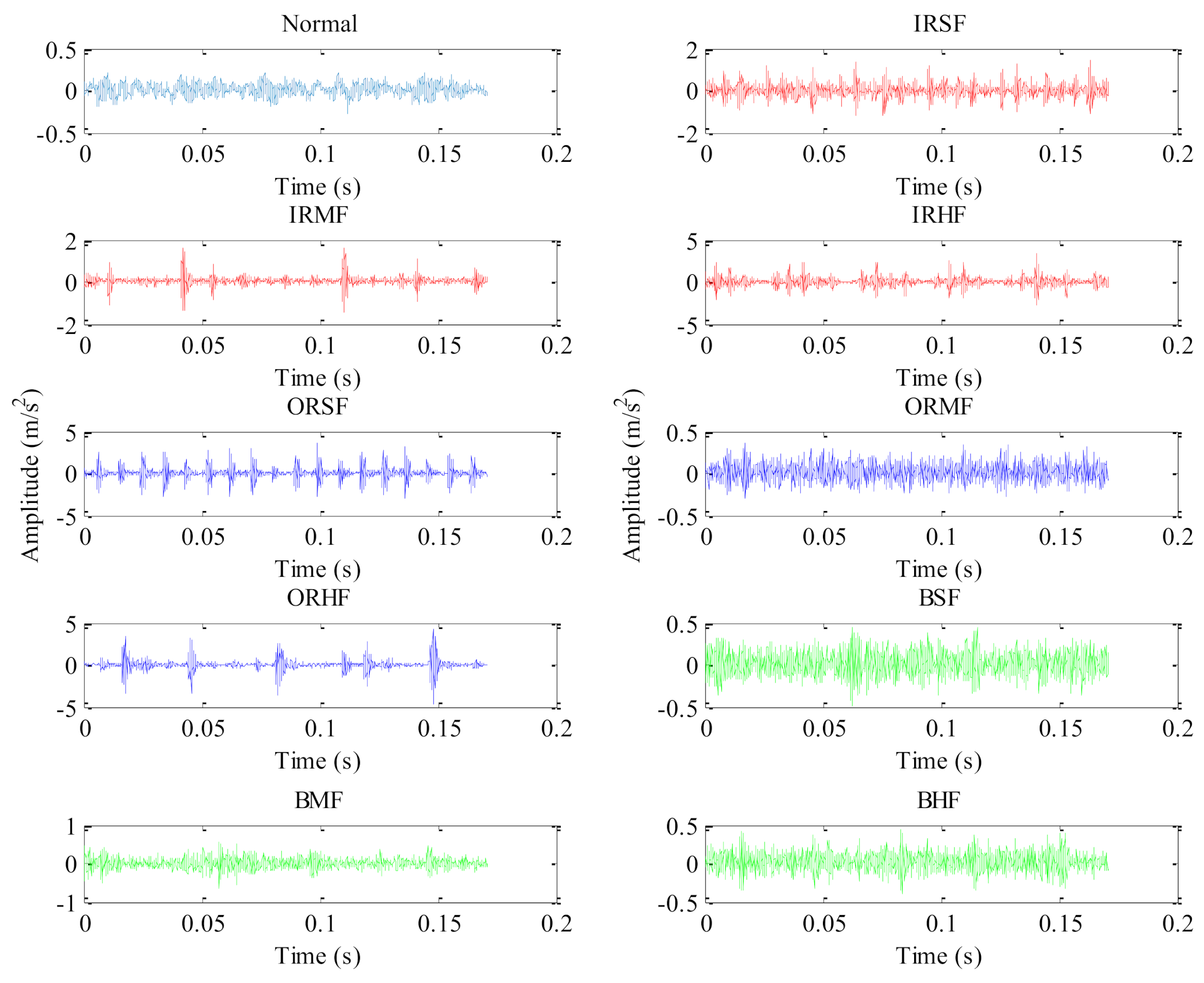
| Normal | NORM | 0 | 25 | 25 | 1 |
| Inner race slight fault | IRSF | 0.007 | 25 | 25 | 2 |
| Inner race medium fault | IRMF | 0.014 | 25 | 25 | 3 |
| Inner race heavy fault | IRHF | 0.021 | 25 | 25 | 4 |
| Outer race slight fault | ORSF | 0.007 | 25 | 25 | 5 |
| Outer race medium fault | ORMF | 0.014 | 25 | 25 | 6 |
| Outer race heavy fault | ORHF | 0.021 | 25 | 25 | 7 |
| Ball slight fault | BSF | 0.007 | 25 | 25 | 8 |
| Ball medium fault | BMF | 0.014 | 25 | 25 | 9 |
| Ball heavy fault | BHF | 0.021 | 25 | 25 | 10 |
| Parameter Setting of HMFE | Identification Accuracy (%) | ||
|---|---|---|---|
| The Embedded Dimension m | The Decomposition Level k | The Scale Factor τ | |
| 1 | 2 | 4 | 87.60 |
| 2 | 2 | 6 | 93.20 |
| 2 | 3 | 7 | 96.80 |
| 3 | 3 | 7 | 98.80 |
| 3 | 3 | 8 | 100 |
| 4 | 3 | 8 | 99.20 |
| 4 | 4 | 12 | 98.40 |
| 5 | 4 | 16 | 98.80 |
| Classifier | Identification Accuracy Obtained by Combining HMFE and Different Classifier Methods in 5 Trials | Average Accuracy (%) | ||||
|---|---|---|---|---|---|---|
| 1 | 2 | 3 | 4 | 5 | ||
| SMM | 100 | 99.60 | 100 | 100 | 100 | 99.92 |
| SVM | 97.60 | 98.00 | 97.60 | 97.60 | 97.20 | 97.60 |
| ELM | 98.40 | 98.80 | 98.40 | 98.00 | 98.40 | 98.40 |
| BPNN | 96.40 | 96.80 | 96.40 | 97.20 | 96.80 | 96.72 |
| Methods | The Optimal Parameter Setting |
|---|---|
| HMFE | The embedded dimension m = 3, the decomposition level k = 3, and the scale factor τ = 8, the similarity tolerance , where SD is the standard deviation of the original signal. |
| HFE | The embedded dimension m = 3, the decomposition level k = 3, the similarity tolerance , where SD is the standard deviation of the original signal. |
| MFE | The embedded dimension m = 3, the scale factor τ = 10, the similarity tolerance , where SD is the standard deviation of the original signal. |
| RCMDE | The embedded dimension m = 3, time delay d = 1, the number of classes c = 5, the scale factor τ = 10. |
| GCMPE | The embedded dimension m = 3, time delay d = 1, the scale factor τ = 12. |
| GRCMSE | The embedded dimension m = 3, the scale factor τ = 10, the similarity tolerance , where SD is the standard deviation of the original signal. |
| HSE | The embedded dimension m = 3, the decomposition level k = 3, the similarity tolerance , where SD is the standard deviation of the original signal. |
| Methods | Maximum Accuracy (%) | Minimum Accuracy (%) | Average Accuracy (%) | Standard Deviation |
|---|---|---|---|---|
| HMFE | 100 | 99.60 | 99.92 | 0.1687 |
| HFE | 97.60 | 96.80 | 97.08 | 0.2700 |
| MFE | 96.00 | 95.20 | 95.44 | 0.3373 |
| RCMDE | 98.00 | 97.20 | 97.72 | 0.2700 |
| GCMPE | 96.80 | 96.00 | 96.20 | 0.2828 |
| GRCMSE | 94.80 | 94.00 | 94.28 | 0.3293 |
| HSE | 92.40 | 91.60 | 91.92 | 0.2530 |
| Bearing Type | Ball Diameter (mm) | Pitch Diameter (mm) | Number of Balls | Contact Angle (°) |
|---|---|---|---|---|
| HRB6205 | 7.94 | 39.04 | 9 | 0 |
| Bearing Health Conditions | Abbreviation | Number of Training Samples | Number of Testing Samples | Class Labels |
|---|---|---|---|---|
| Normal | NORM | 30 | 30 | 1 |
| Outer race fault | ORF | 30 | 30 | 2 |
| Inner race fault | IRF | 30 | 30 | 3 |
| Ball fault | BF | 30 | 30 | 4 |
| Outer and inner race compound fault | OIRCF | 30 | 30 | 5 |
| Outer race and ball compound fault | ORBCF | 30 | 30 | 6 |
| Parameter Setting of HMFE | Identification Accuracy (%) | ||
|---|---|---|---|
| The Embedded Dimension m | The Decomposition Level k | The Scale Factor τ | |
| 1 | 2 | 4 | 89.44 |
| 2 | 2 | 6 | 93.33 |
| 2 | 3 | 7 | 97.22 |
| 3 | 3 | 7 | 98.33 |
| 3 | 3 | 8 | 99.44 |
| 4 | 3 | 8 | 100 |
| 4 | 4 | 12 | 98.33 |
| 5 | 4 | 16 | 98.89 |
| Classifier | Identification Accuracy Obtained by Combining HMFE and Different Classifier Methods in 5 Trials | Average Accuracy (%) | ||||
|---|---|---|---|---|---|---|
| 1 | 2 | 3 | 4 | 5 | ||
| SMM | 100 | 100 | 99.44 | 100 | 99.44 | 99.77 |
| SVM | 97.22 | 96.67 | 97.22 | 96.67 | 96.11 | 96.78 |
| ELM | 98.33 | 97.78 | 98.33 | 97.22 | 98.33 | 97.99 |
| BPNN | 95.55 | 96.11 | 95.55 | 96.11 | 95.00 | 95.66 |
| Methods | The Optimal Parameter Setting |
|---|---|
| HMFE | The embedded dimension m = 4, the decomposition level k = 3, and the scale factor τ = 8, the similarity tolerance , where SD is the standard deviation of the original signal. |
| HFE | The embedded dimension m = 4, the decomposition level k = 3, the similarity tolerance , where SD is the standard deviation of the original signal. |
| MFE | The embedded dimension m = 3, the scale factor τ = 12, the similarity tolerance , where SD is the standard deviation of the original signal. |
| RCMDE | The embedded dimension m = 3, time delay d = 1, the number of classes c = 6, the scale factor τ = 12. |
| GCMPE | The embedded dimension m = 3, time delay d = 1, the scale factor τ = 15. |
| GRCMSE | The embedded dimension m = 4, the scale factor τ = 10, the similarity tolerance , where SD is the standard deviation of the original signal. |
| HSE | The embedded dimension m = 3, the decomposition level k = 3, the similarity tolerance , where SD is the standard deviation of the original signal. |
| Methods | Maximum Accuracy (%) | Minimum Accuracy (%) | Average Accuracy (%) | Standard Deviation |
|---|---|---|---|---|
| HMFE | 100 | 99.44 | 99.83 | 0.2705 |
| HFE | 96.67 | 95.55 | 96.27 | 0.3780 |
| MFE | 94.44 | 93.33 | 94.16 | 0.3913 |
| RCMDE | 96.67 | 95.55 | 96.16 | 0.4132 |
| GCMPE | 95.55 | 94.44 | 94.83 | 0.3758 |
| GRCMSE | 92.77 | 91.67 | 92.22 | 0.3667 |
| HSE | 90.55 | 89.40 | 90.04 | 0.4226 |
Publisher’s Note: MDPI stays neutral with regard to jurisdictional claims in published maps and institutional affiliations. |
© 2021 by the authors. Licensee MDPI, Basel, Switzerland. This article is an open access article distributed under the terms and conditions of the Creative Commons Attribution (CC BY) license (https://creativecommons.org/licenses/by/4.0/).
Share and Cite
Yan, X.; Xu, Y.; Jia, M. Intelligent Fault Diagnosis of Rolling-Element Bearings Using a Self-Adaptive Hierarchical Multiscale Fuzzy Entropy. Entropy 2021, 23, 1128. https://doi.org/10.3390/e23091128
Yan X, Xu Y, Jia M. Intelligent Fault Diagnosis of Rolling-Element Bearings Using a Self-Adaptive Hierarchical Multiscale Fuzzy Entropy. Entropy. 2021; 23(9):1128. https://doi.org/10.3390/e23091128
Chicago/Turabian StyleYan, Xiaoan, Yadong Xu, and Minping Jia. 2021. "Intelligent Fault Diagnosis of Rolling-Element Bearings Using a Self-Adaptive Hierarchical Multiscale Fuzzy Entropy" Entropy 23, no. 9: 1128. https://doi.org/10.3390/e23091128