
Analysis of Pseudo-Lyapunov Exponents of Solar Convection Using State-of-the-Art Observations

 , , , ,
  ,
, 
Abstract
:1. Introduction
2. Observations and Data Analysis
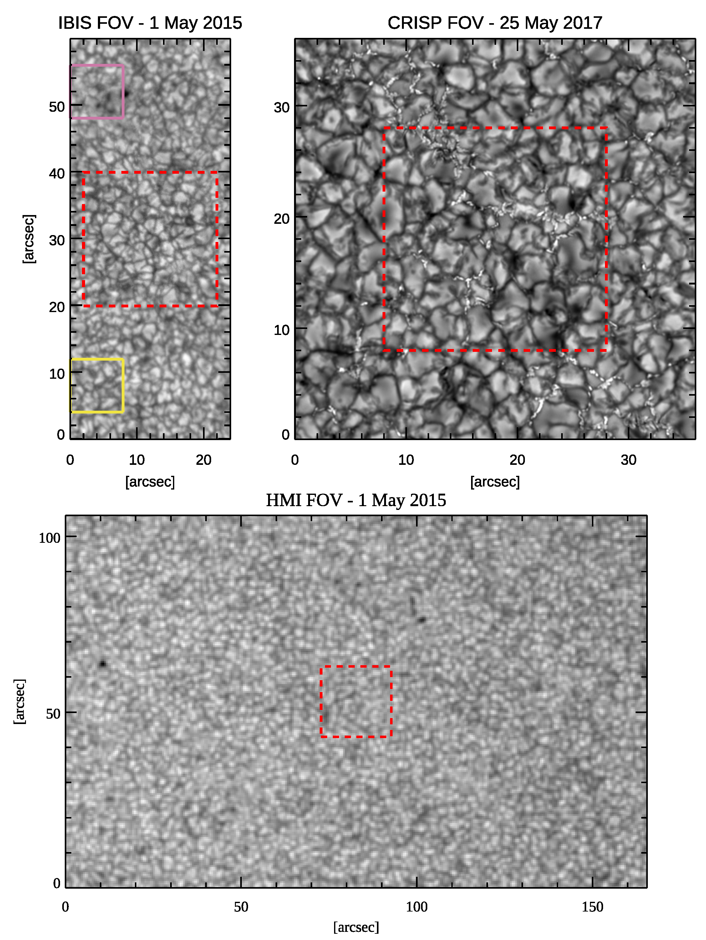
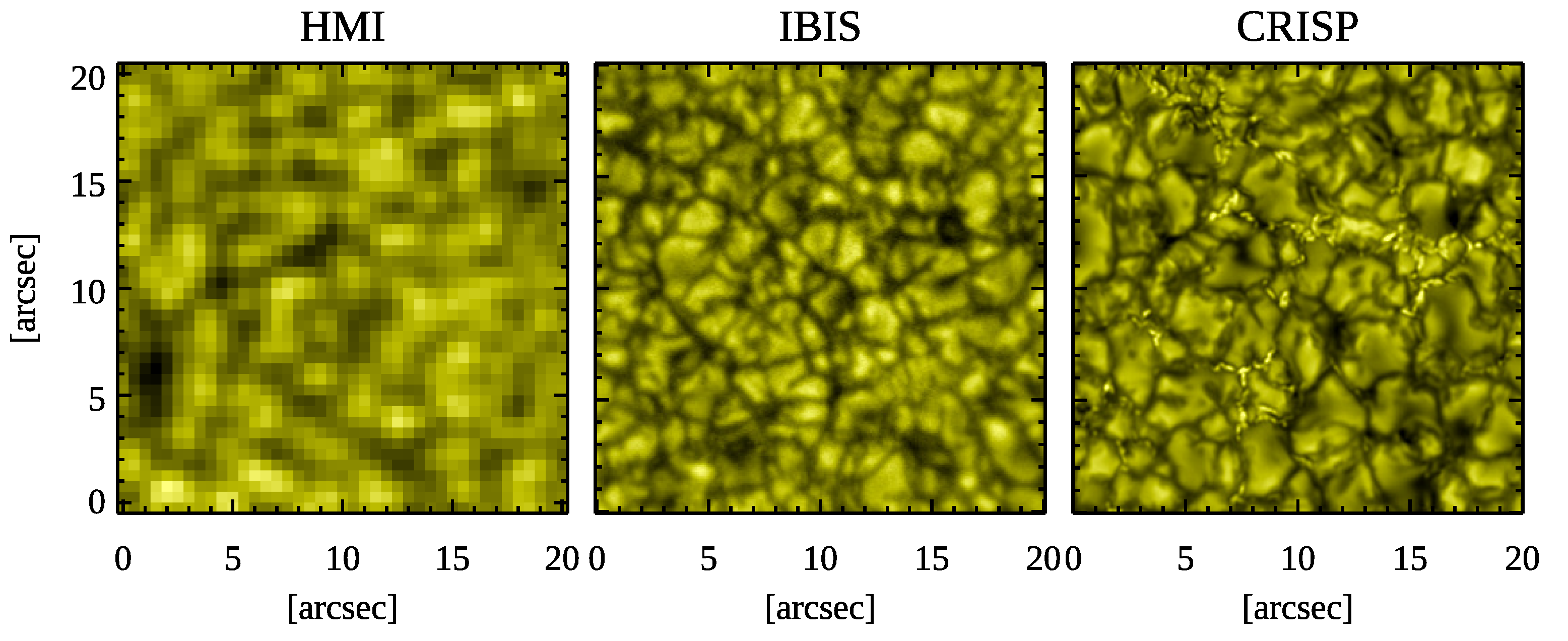
2.1. Observations
2.2. Data Analysis
- Continuum intensity fluctuations, hereafter referred to as , which are associated with the temperature differences between hotter granules and cooler intergranular lanes in the observed region;
- Line-of-sight (LoS) velocity fluctuations, hereafter referred to as , which are related to velocity differences between the upward and downward plasma motions in the studied region, and are encoded in the Doppler shift of the observed spectral lines;
- Full width at half maximum () fluctuations, hereafter referred to as , which convey information about changes of the non-thermal motions in the observed region, contributing to the broadening of the spectral line profiles, as for turbulent motions (e.g., [14]);
- Bisector variations of the line profiles associated with the vertical velocity gradients in the observed region; these variations are evaluated using the definition of the line asymmetry parameter A reported in Hanslmeier et al. [74], and are hereafter referred to as .
3. Results
3.1. Further Analyses
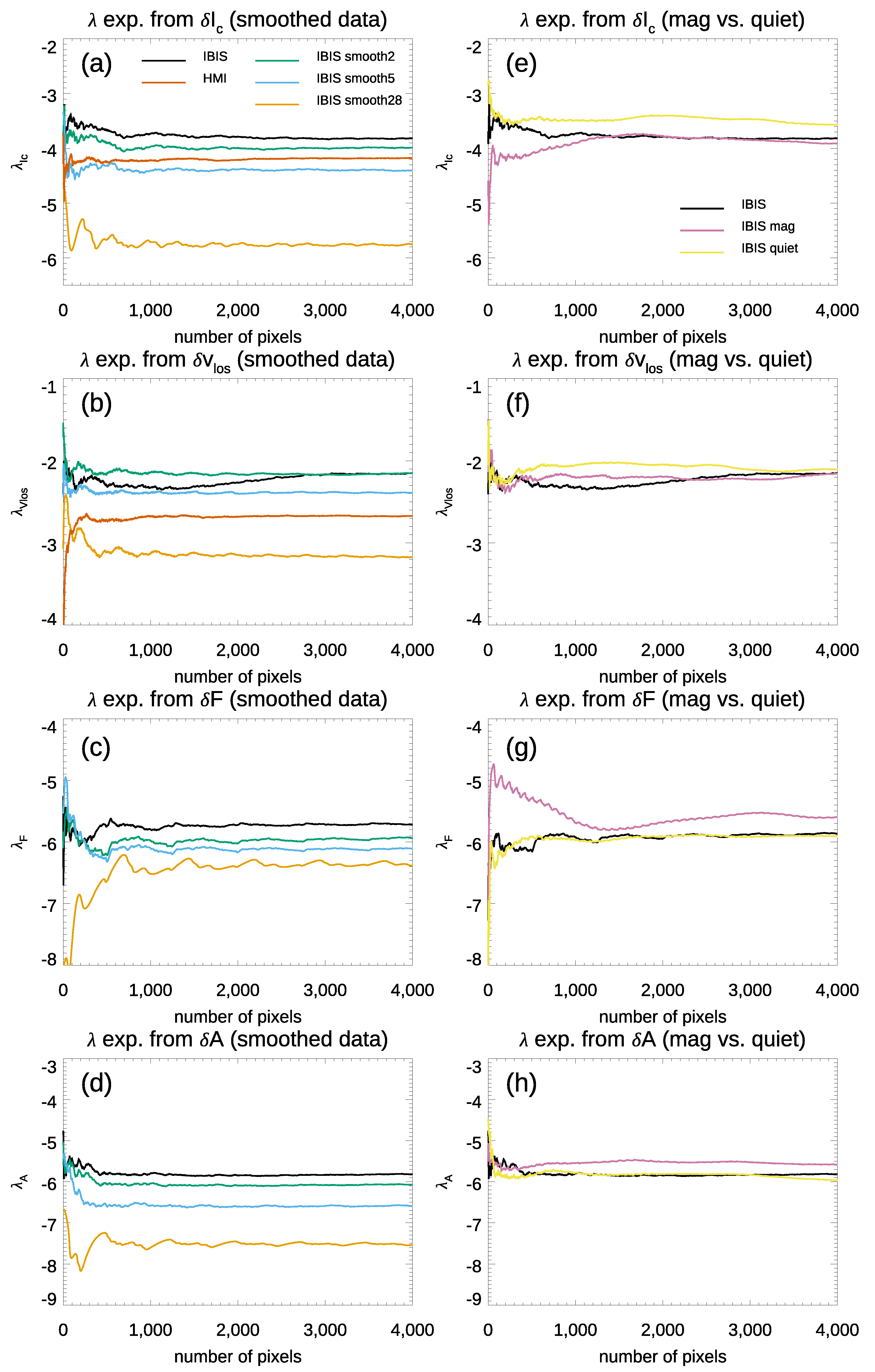
- Subgranular, corresponding to a spatial resolution of 0.36″ ( pixels kernel);
- Granular, corresponding to a spatial resolution of 0.90″ ( pixels kernel);
- Mesogranular, corresponding to a spatial resolution of 5.04″ ( pixels kernel).
4. Comments and Conclusions
Author Contributions
Funding
Data Availability Statement
Acknowledgments
Conflicts of Interest
Abbreviations
| Ra | Rayleigh number |
| IBIS | Interferometric Bidimensional Spectrometer |
| DST | Dunn Solar Telescope |
| CRISP | Crisp Imaging SpectroPolarimeter |
| SST | Swedish 1 m Solar Telescope |
| HMI | Helioseismic and Magnetic Imager |
| SDO | Solar Dynamic Observatory |
| SHARPs | Space-Weather HMI Active Region Patches |
| FoV | Field-of-view |
| MOMFBD | Multi-Object Multi-Frame Blind Deconvolution |
| AO | Adaptive optics |
| MHD | Magnetohydrodynamic |
References
- Niemela, J.J.; Skrbek, L.; Sreenivasan, K.R.; Donnelly, R.J. Turbulent convection at very high Rayleigh numbers. Nature 2000, 404, 837–840. [Google Scholar] [CrossRef]
- Nordlund, Å.; Stein, R.F.; Asplund, M. Solar Surface Convection. Living Rev. Sol. Phys. 2009, 6, 2. [Google Scholar] [CrossRef] [Green Version]
- Herschel, W. Observations Tending to Investigate the Nature of the Sun, in Order to Find the Causes or Symptoms of Its Variable Emission of Light and Heat; With Remarks on the Use That May Possibly Be Drawn from Solar Observations. Philos. Trans. R. Soc. Lond. Ser. I 1801, 91, 265–318. [Google Scholar]
- Rimmele, T.R. Status of the Daniel K. Inouye Solar Telescope. In Proceedings of the American Astronomical Society Meeting Abstracts #234, St. Louis, MO, USA, 9–13 June 2019; Volume 234, p. 226.01. [Google Scholar]
- Johnston, H. Convection cells the size of Texas dazzle with clarity on the Sun. Phys. World 2020, 33, 10. [Google Scholar] [CrossRef]
- Löfdahl, M.G. Multi-frame blind deconvolution with linear equality constraints. In Image Reconstruction from Incomplete Data II; Bones, P.J., Fiddy, M.A., Millane, R.P., Eds.; Society of Photo-Optical Instrumentation Engineers (SPIE) Conference Series; SPIE: Bellingham, WA, USA, 2002; Volume 4792, pp. 146–155. [Google Scholar] [CrossRef] [Green Version]
- Hirzberger, J.; Vázquez, M.; Bonet, J.A.; Hanslmeier, A.; Sobotka, M. Time Series of Solar Granulation Images. I. Differences between Small and Large Granules in Quiet Regions. Astrophys. J. 1997, 480, 406–419. [Google Scholar] [CrossRef]
- Hirzberger, J.; Bonet, J.A.; Vázquez, M.; Hanslmeier, A. Time Series of Solar Granulation Images. II. Evolution of Individual Granules. Astrophys. J. 1999, 515, 441–454. [Google Scholar] [CrossRef]
- Lemmerer, B.; Hanslmeier, A.; Muthsam, H.; Piantschitsch, I. Dynamics of small-scale convective motions. Astron. Astrophys. 2017, 598, A126. [Google Scholar] [CrossRef] [Green Version]
- Muller, R.; Auffret, H.; Roudier, T.; Vigneau, J.; Simon, G.W.; Frank, Z.; Shine, R.A.; Title, A.M. Evolution and advection of solar mesogranulation. Nature 1992, 356, 322–325. [Google Scholar] [CrossRef]
- Oba, T.; Iida, Y.; Shimizu, T. Height-dependent Velocity Structure of Photospheric Convection in Granules and Intergranular Lanes with Hinode/SOT. Astrophys. J. 2017, 836, 40. [Google Scholar] [CrossRef] [Green Version]
- Oba, T.; Riethmüller, T.L.; Solanki, S.K.; Iida, Y.; Quintero Noda, C.; Shimizu, T. The Small-scale Structure of Photospheric Convection Retrieved by a Deconvolution Technique Applied to Hinode/SP Data. Astrophys. J. 2017, 849, 7. [Google Scholar] [CrossRef] [Green Version]
- Khomenko, E.; Martínez Pillet, V.; Solanki, S.K.; del Toro Iniesta, J.C.; Gandorfer, A.; Bonet, J.A.; Domingo, V.; Schmidt, W.; Barthol, P.; Knölker, M. Where the Granular Flows Bend. Astrophys. J. Lett. 2010, 723, L159–L163. [Google Scholar] [CrossRef] [Green Version]
- Ishikawa, R.T.; Katsukawa, Y.; Oba, T.; Nakata, M.; Nagaoka, K.; Kobayashi, T. Study of the Dynamics of Convective Turbulence in the Solar Granulation by Spectral Line Broadening and Asymmetry. Astrophys. J. 2020, 890, 138. [Google Scholar] [CrossRef]
- November, L.J.; Toomre, J.; Gebbie, K.B.; Simon, G.W. The detection of mesogranulation on the sun. Astrophys. J. Lett. 1981, 245, L123–L126. [Google Scholar] [CrossRef]
- Brandt, P.N.; Ferguson, S.; Shine, R.A.; Tarbell, T.D.; Scharmer, G.B. Variation of granulation properties on a mesogranular scale. Astron. Astrophys. 1991, 241, 219–226. [Google Scholar]
- Domínguez Cerdeña, I. Evidence of mesogranulation from magnetograms of the Sun. Astron. Astrophys. 2003, 412, L65–L68. [Google Scholar] [CrossRef]
- Leitzinger, M.; Brandt, P.N.; Hanslmeier, A.; Pötzi, W.; Hirzberger, J. Dynamics of solar mesogranulation. Astron. Astrophys. 2005, 444, 245–255. [Google Scholar] [CrossRef]
- Rast, M.P. The Scales of Granulation, Mesogranulation, and Supergranulation. Astrophys. J. 2003, 597, 1200–1210. [Google Scholar] [CrossRef]
- Berrilli, F.; Del Moro, D.; Consolini, G.; Pietropaolo, E.; Duvall, T.L.J.; Kosovichev, A.G. Structure Properties of Supergranulation and Granulation. Sol. Phys. 2004, 221, 33–45. [Google Scholar] [CrossRef]
- Del Moro, D.; Berrilli, F.; Duvall, T.L.J.; Kosovichev, A.G. Dynamics and Structure of Supergranulation. Sol. Phys. 2004, 221, 23–32. [Google Scholar] [CrossRef]
- Rincon, F.; Rieutord, M. The Sun’s supergranulation. Living Rev. Sol. Phys. 2018, 15, 6. [Google Scholar] [CrossRef] [Green Version]
- Beck, J.G.; Duvall, T.L.; Scherrer, P.H. Long-lived giant cells detected at the surface of the Sun. Nature 1998, 394, 653–655. [Google Scholar] [CrossRef]
- Hathaway, D.H.; Upton, L.; Colegrove, O. Giant Convection Cells Found on the Sun. Science 2013, 342, 1217–1219. [Google Scholar] [CrossRef] [Green Version]
- McIntosh, S.W.; Wang, X.; Leamon, R.J.; Scherrer, P.H. Identifying Potential Markers of the Sun’s Giant Convective Scale. Astrophys. J. Lett. 2014, 784, L32. [Google Scholar] [CrossRef] [Green Version]
- Rieutord, M.; Roudier, T.; Malherbe, J.M.; Rincon, F. On mesogranulation, network formation and supergranulation. Astron. Astrophys. 2000, 357, 1063–1072. [Google Scholar]
- Charbonneau, P. Dynamo models of the solar cycle. Living Rev. Sol. Phys. 2020, 17, 4. [Google Scholar] [CrossRef]
- Stein, R.F. Solar Surface Magneto-Convection. Living Rev. Sol. Phys. 2012, 9, 4. [Google Scholar] [CrossRef] [Green Version]
- Bellot Rubio, L.; Orozco Suárez, D. Quiet Sun magnetic fields: An observational view. Living Rev. Sol. Phys. 2019, 16, 1. [Google Scholar] [CrossRef] [Green Version]
- Centeno, R.; Socas-Navarro, H.; Lites, B.; Kubo, M.; Frank, Z.; Shine, R.; Tarbell, T.; Title, A.; Ichimoto, K.; Tsuneta, S.; et al. Emergence of Small-Scale Magnetic Loops in the Quiet-Sun Internetwork. Astrophys. J. Lett. 2007, 666, L137–L140. [Google Scholar] [CrossRef] [Green Version]
- Orozco Suárez, D.; Bellot Rubio, L.R.; del Toro Iniesta, J.C.; Tsuneta, S. Magnetic field emergence in quiet Sun granules. Astron. Astrophys. 2008, 481, L33–L36. [Google Scholar] [CrossRef] [Green Version]
- Viticchié, B. On the Polarimetric Signature of Emerging Magnetic Loops in the Quiet Sun. Astrophys. J. Lett. 2012, 747, L36. [Google Scholar] [CrossRef]
- Giannattasio, F.; Del Moro, D.; Berrilli, F.; Bellot Rubio, L.; Gošić, M.; Orozco Suárez, D. Diffusion of Solar Magnetic Elements up to Supergranular Spatial and Temporal Scales. Astrophys. J. Lett. 2013, 770, L36. [Google Scholar] [CrossRef]
- Giannattasio, F.; Stangalini, M.; Berrilli, F.; Del Moro, D.; Bellot Rubio, L. Diffusion of Magnetic Elements in a Supergranular Cell. Astrophys. J. 2014, 788, 137. [Google Scholar] [CrossRef] [Green Version]
- Jafarzadeh, S.; Solanki, S.K.; Cameron, R.H.; Barthol, P.; Blanco Rodríguez, J.; del Toro Iniesta, J.C.; Gandorfer, A.; Gizon, L.; Hirzberger, J.; Knölker, M.; et al. Kinematics of Magnetic Bright Features in the Solar Photosphere. Astrophys. J. Suppl. Ser. 2017, 229, 8. [Google Scholar] [CrossRef] [Green Version]
- Lites, B.W.; Leka, K.D.; Skumanich, A.; Martinez Pillet, V.; Shimizu, T. Small-Scale Horizontal Magnetic Fields in the Solar Photosphere. Astrophys. J. 1996, 460, 1019. [Google Scholar] [CrossRef]
- Lites, B.W.; Kubo, M.; Socas-Navarro, H.; Berger, T.; Frank, Z.; Shine, R.; Tarbell, T.; Title, A.; Ichimoto, K.; Katsukawa, Y.; et al. The Horizontal Magnetic Flux of the Quiet-Sun Internetwork as Observed with the Hinode Spectro-Polarimeter. Astrophys. J. 2008, 672, 1237–1253. [Google Scholar] [CrossRef]
- Danilovic, S.; Beeck, B.; Pietarila, A.; Schüssler, M.; Solanki, S.K.; Martínez Pillet, V.; Bonet, J.A.; del Toro Iniesta, J.C.; Domingo, V.; Barthol, P.; et al. Transverse Component of the Magnetic Field in the Solar Photosphere Observed by SUNRISE. Astrophys. J. Lett. 2010, 723, L149–L153. [Google Scholar] [CrossRef] [Green Version]
- Kianfar, S.; Jafarzadeh, S.; Mirtorabi, M.T.; Riethmüller, T.L. Linear Polarization Features in the Quiet-Sun Photosphere: Structure and Dynamics. Sol. Phys. 2018, 293, 123. [Google Scholar] [CrossRef] [PubMed] [Green Version]
- Martínez González, M.J.; Bellot Rubio, L.R. Emergence of Small-scale Magnetic Loops Through the Quiet Solar Atmosphere. Astrophys. J. 2009, 700, 1391–1403. [Google Scholar] [CrossRef] [Green Version]
- Guglielmino, S.L.; Martínez Pillet, V.; Bonet, J.A.; del Toro Iniesta, J.C.; Bellot Rubio, L.R.; Solanki, S.K.; Schmidt, W.; Gandorfer, A.; Barthol, P.; Knölker, M. The Frontier between Small-scale Bipoles and Ephemeral Regions in the Solar Photosphere: Emergence and Decay of an Intermediate-scale Bipole Observed with SUNRISE/IMaX. Astrophys. J. 2012, 745, 160. [Google Scholar] [CrossRef]
- Fischer, C.E.; Borrero, J.M.; Bello González, N.; Kaithakkal, A.J. Observations of solar small-scale magnetic flux-sheet emergence. Astron. Astrophys. 2019, 622, L12. [Google Scholar] [CrossRef]
- Guglielmino, S.L.; Pillet, V.M.; Ruiz Cobo, B.; Bellot Rubio, L.R.; del Toro Iniesta, J.C.; Solanki, S.K.; Riethmüller, T.L.; Zuccarello, F. On the Magnetic Nature of an Exploding Granule as Revealed by Sunrise/IMaX. Astrophys. J. 2020, 896, 62. [Google Scholar] [CrossRef]
- Falco, M.; Puglisi, G.; Guglielmino, S.L.; Romano, P.; Ermolli, I.; Zuccarello, F. Comparison of different populations of granular features in the solar photosphere. Astron. Astrophys. 2017, 605, A87. [Google Scholar] [CrossRef]
- Nesis, A.; Hammer, R.; Roth, M.; Schleicher, H. Dynamics of the solar granulation. VII. A nonlinear approach. Astron. Astrophys. 2001, 373, 307–317. [Google Scholar] [CrossRef]
- Viavattene, G.; Consolini, G.; Giovannelli, L.; Berrilli, F.; Del Moro, D.; Giannattasio, F.; Penza, V.; Calchetti, D. Testing the Steady-State Fluctuation Relation in the Solar Photospheric Convection. Entropy 2020, 22, 716. [Google Scholar] [CrossRef] [PubMed]
- Gudiksen, B.V.; Carlsson, M.; Hansteen, V.H.; Hayek, W.; Leenaarts, J.; Martínez-Sykora, J. The stellar atmosphere simulation code Bifrost. Code description and validation. Astron. Astrophys. 2011, 531, A154. [Google Scholar] [CrossRef] [Green Version]
- Beeck, B.; Collet, R.; Steffen, M.; Asplund, M.; Cameron, R.H.; Freytag, B.; Hayek, W.; Ludwig, H.G.; Schüssler, M. Simulations of the solar near-surface layers with the CO5BOLD, MURaM, and Stagger codes. Astron. Astrophys. 2012, 539, A121. [Google Scholar] [CrossRef] [Green Version]
- Freytag, B.; Steffen, M.; Ludwig, H.G.; Wedemeyer-Böhm, S.; Schaffenberger, W.; Steiner, O. Simulations of stellar convection with CO5BOLD. J. Comput. Phys. 2012, 231, 919–959. [Google Scholar] [CrossRef] [Green Version]
- Goldreich, P.; Kumar, P. Wave Generation by Turbulent Convection. Astrophys. J. 1990, 363, 694. [Google Scholar] [CrossRef]
- Carlsson, M.; De Pontieu, B.; Hansteen, V.H. New View of the Solar Chromosphere. Annu. Rev. Astron. Astrophys. 2019, 57, 189–226. [Google Scholar] [CrossRef]
- Malherbe, J.M.; Roudier, T.; Rieutord, M.; Berger, T.; Franck, Z. Acoustic Events in the Solar Atmosphere from Hinode/SOT NFI Observations. Sol. Phys. 2012, 278, 241–256. [Google Scholar] [CrossRef] [Green Version]
- Malherbe, J.M.; Roudier, T.; Frank, Z.; Rieutord, M. Families of Granules, Flows, and Acoustic Events in the Solar Atmosphere from Hinode Observations. Sol. Phys. 2015, 290, 321–333. [Google Scholar] [CrossRef]
- Kayshap, P.; Murawski, K.; Srivastava, A.K.; Musielak, Z.E.; Dwivedi, B.N. Vertical propagation of acoustic waves in the solar internetworkas observed by IRIS. Mon. Not. R. Astron. Soc. 2018, 479, 5512–5521. [Google Scholar] [CrossRef]
- Morton, R.J.; Verth, G.; Hillier, A.; Erdélyi, R. The Generation and Damping of Propagating MHD Kink Waves in the Solar Atmosphere. Astrophys. J. 2014, 784, 29. [Google Scholar] [CrossRef] [Green Version]
- Stangalini, M.; Consolini, G.; Berrilli, F.; De Michelis, P.; Tozzi, R. Observational evidence for buffeting-induced kink waves in solar magnetic elements. Astron. Astrophys. 2014, 569, A102. [Google Scholar] [CrossRef] [Green Version]
- Stangalini, M.; Giannattasio, F.; Erdélyi, R.; Jafarzadeh, S.; Consolini, G.; Criscuoli, S.; Ermolli, I.; Guglielmino, S.L.; Zuccarello, F. Polarized Kink Waves in Magnetic Elements: Evidence for Chromospheric Helical Waves. Astrophys. J. 2017, 840, 19. [Google Scholar] [CrossRef] [Green Version]
- Kurths, J.; Brandenburg, A. Lyapunov exponents for hydromagnetic convection. Phys. Rev. A 1991, 44, R3427–R3429. [Google Scholar] [CrossRef]
- Steffen, M.; Freytag, B. Lyapunov exponents for solar surface convection. Chaos Solitons Fractals 1995, 5, 1965–1973. [Google Scholar] [CrossRef]
- Hanslmeier, A.; Nesis, A. Non linear dynamics of the solar granulation: A first approach. Astron. Astrophys. 1994, 286, 263–268. [Google Scholar]
- Nagashima, K.; Löptien, B.; Gizon, L.; Birch, A.C.; Cameron, R.; Couvidat, S.; Danilovic, S.; Fleck, B.; Stein, R. Interpreting the Helioseismic and Magnetic Imager (HMI) Multi-Height Velocity Measurements. Sol. Phys. 2014, 289, 3457–3481. [Google Scholar] [CrossRef] [Green Version]
- Jafarzadeh, S.; Rouppe van der Voort, L.; de la Cruz Rodríguez, J. Magnetic Upflow Events in the Quiet-Sun Photosphere. I. Observations. Astrophys. J. 2015, 810, 54. [Google Scholar] [CrossRef] [Green Version]
- Cavallini, F. IBIS: A New Post-Focus Instrument for Solar Imaging Spectroscopy. Sol. Phys. 2006, 236, 415–439. [Google Scholar] [CrossRef] [Green Version]
- Ermolli, I.; Cristaldi, A.; Giorgi, F.; Giannattasio, F.; Stangalini, M.; Romano, P.; Tritschler, A.; Zuccarello, F. Plasma flows and magnetic field interplay during the formation of a pore. Astron. Astrophys. 2017, 600, A102. [Google Scholar] [CrossRef] [Green Version]
- Murabito, M.; Ermolli, I.; Giorgi, F.; Stangalini, M.; Guglielmino, S.L.; Jafarzadeh, S.; Socas-Navarro, H.; Romano, P.; Zuccarello, F. Height Dependence of the Penumbral Fine-scale Structure in the Inner Solar Atmosphere. Astrophys. J. 2019, 873, 126. [Google Scholar] [CrossRef] [Green Version]
- Van Noort, M.; Rouppe van der Voort, L.; Löfdahl, M.G. Solar Image Restoration By Use Of Multi-frame Blind De-convolution With Multiple Objects And Phase Diversity. Sol. Phys. 2005, 228, 191–215. [Google Scholar] [CrossRef]
- Murabito, M.; Shetye, J.; Stangalini, M.; Verwichte, E.; Arber, T.; Ermolli, I.; Giorgi, F.; Goffrey, T. Unveiling the magnetic nature of chromospheric vortices. Astron. Astrophys. 2020, 639, 59. [Google Scholar] [CrossRef]
- Scharmer, G.B. Comments on the optimization of high resolution Fabry-Pérot filtergraphs. Astron. Astrophys. 2006, 447, 1111–1120. [Google Scholar] [CrossRef]
- De la Cruz Rodríguez, J.; Löfdahl, M.G.; Sütterlin, P.; Hillberg, T.; Rouppe van der Voort, L. CRISPRED: A data pipeline for the CRISP imaging spectropolarimeter. Astron. Astrophys. 2015, 573, A40. [Google Scholar] [CrossRef]
- Bose, S.; Henriques, V.M.J.; Joshi, J.; Rouppe van der Voort, L. Characterization and formation of on-disk spicules in the Ca II K and Mg II k spectral lines. Astron. Astrophys. 2019, 631, L5. [Google Scholar] [CrossRef]
- Bose, S.; Joshi, J.; Henriques, V.M.J.; Rouppe van der Voort, L. Spicules and downflows in the solar chromosphere. arXiv 2021, arXiv:2101.07829. [Google Scholar]
- Scherrer, P.H.; Schou, J.; Bush, R.I.; Kosovichev, A.G.; Bogart, R.S.; Hoeksema, J.T.; Liu, Y.; Duvall, T.L.; Zhao, J.; Title, A.M.; et al. The Helioseismic and Magnetic Imager (HMI) Investigation for the Solar Dynamics Observatory (SDO). Sol. Phys. 2012, 275, 207–227. [Google Scholar] [CrossRef] [Green Version]
- Pesnell, W.D.; Thompson, B.J.; Chamberlin, P.C. The Solar Dynamics Observatory (SDO). Sol. Phys. 2012, 275, 3–15. [Google Scholar] [CrossRef] [Green Version]
- Hanslmeier, A.; Mattig, W.; Nesis, A. High spatial resolution observations of some solar photospheric line profiles. Astron. Astrophys. 1990, 238, 354–362. [Google Scholar]
- Murabito, M.; Romano, P.; Guglielmino, S.L.; Zuccarello, F. On the Formation of a Stable Penumbra in a Region of Flux Emergence in the Sun. Astrophys. J. 2017, 834, 76. [Google Scholar] [CrossRef] [Green Version]
- Martínez González, M.J.; Manso Sainz, R.; Asensio Ramos, A.; Hijano, E. Dead Calm Areas in the Very Quiet Sun. Astrophys. J. 2012, 755, 175. [Google Scholar] [CrossRef] [Green Version]
- Baker, G.L.; Gollub, J.P. Chaotic Dynamics; Cambridge University Press: Cambridge, UK, 1992. [Google Scholar]
- Romano, P.; Berrilli, F.; Criscuoli, S.; Del Moro, D.; Ermolli, I.; Giorgi, F.; Viticchié, B.; Zuccarello, F. A Comparative Analysis of Photospheric Bright Points in an Active Region and in the Quiet Sun. Sol. Phys. 2012, 280, 407–416. [Google Scholar] [CrossRef]
- Tortosa-Andreu, A.; Moreno-Insertis, F. Magnetic flux emergence into the solar photosphere and chromosphere. Astron. Astrophys. 2009, 507, 949–967. [Google Scholar] [CrossRef]
- Guglielmino, S.L.; Bellot Rubio, L.R.; Zuccarello, F.; Aulanier, G.; Vargas Domínguez, S.; Kamio, S. Multiwavelength Observations of Small-scale Reconnection Events Triggered by Magnetic Flux Emergence in the Solar Atmosphere. Astrophys. J. 2010, 724, 1083–1098. [Google Scholar] [CrossRef]
- Guglielmino, S.L.; Zuccarello, F.; Young, P.R.; Murabito, M.; Romano, P. IRIS Observations of Magnetic Interactions in the Solar Atmosphere between Preexisting and Emerging Magnetic Fields. I. Overall Evolution. Astrophys. J. 2018, 856, 127. [Google Scholar] [CrossRef] [Green Version]
- Tsuneta, S.; Ichimoto, K.; Katsukawa, Y.; Nagata, S.; Otsubo, M.; Shimizu, T.; Suematsu, Y.; Nakagiri, M.; Noguchi, M.; Tarbell, T.; et al. The Solar Optical Telescope for the Hinode Mission: An Overview. Sol. Phys. 2008, 249, 167–196. [Google Scholar] [CrossRef]
- Collados, M.; Bettonvil, F.; Cavaller, L.; Ermolli, I.; Gelly, B.; Pérez, A.; Socas-Navarro, H.; Soltau, D.; Volkmer, R.; EST Team. European Solar Telescope: Progress status. Astron. Nachrichten 2010, 331, 615. [Google Scholar] [CrossRef]
- Solanki, S.K.; del Toro Iniesta, J.C.; Woch, J.; Gand orfer, A.; Hirzberger, J.; Alvarez-Herrero, A.; Appourchaux, T.; Martínez Pillet, V.; Pérez-Grand e, I.; Sanchis Kilders, E.; et al. The Polarimetric and Helioseismic Imager on Solar Orbiter. Astron. Astrophys. 2020, 642, A11. [Google Scholar] [CrossRef] [Green Version]
- Müller, D.; St. Cyr, O.C.; Zouganelis, I.; Gilbert, H.R.; Marsden, R.; Nieves-Chinchilla, T.; Antonucci, E.; Auchère, F.; Berghmans, D.; Horbury, T.S.; et al. The Solar Orbiter mission. Science overview. Astron. Astrophys. 2020, 642, A1. [Google Scholar] [CrossRef]


| Telescope | Instrument | Spectral Coverage | Time Coverage | Time Cadence | Spatial Resolution | Formation Height of Line Cores |
|---|---|---|---|---|---|---|
| DST | IBIS | Fe I 617.3 nm | 1 May 2015 14:18–15:03 UT | 48 s | 0.16″ | ∼150 km [61] |
| SST | CRISP | Fe I 630.15 nm | 25 May 2017 09:30–09:40 UT | - | 0.13″ | ∼180 km [62] |
| SDO | HMI | Fe I 617.3 nm | 1 May 2015 14:24 UT 25 May 2017 09:36 UT | - | 1″ | - |
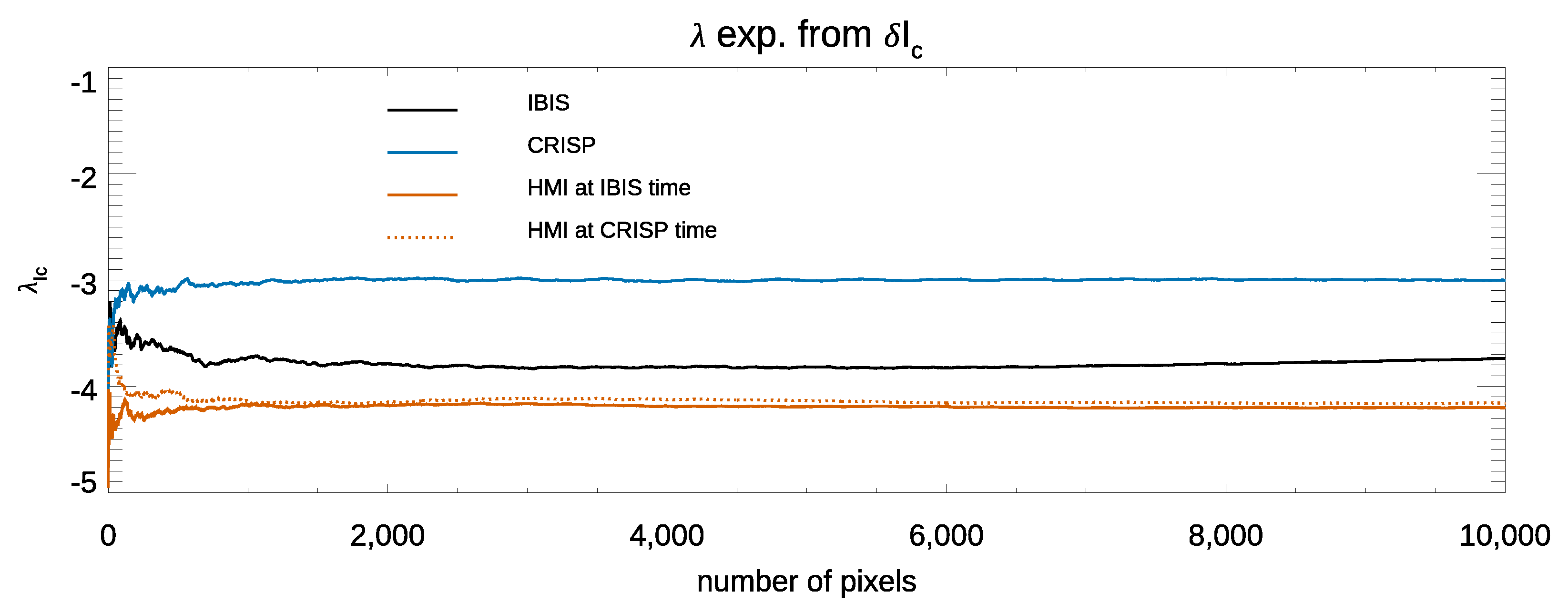
| CRISP | IBIS | HMI at IBIS Time | HMI at CRISP Time | |
|---|---|---|---|---|
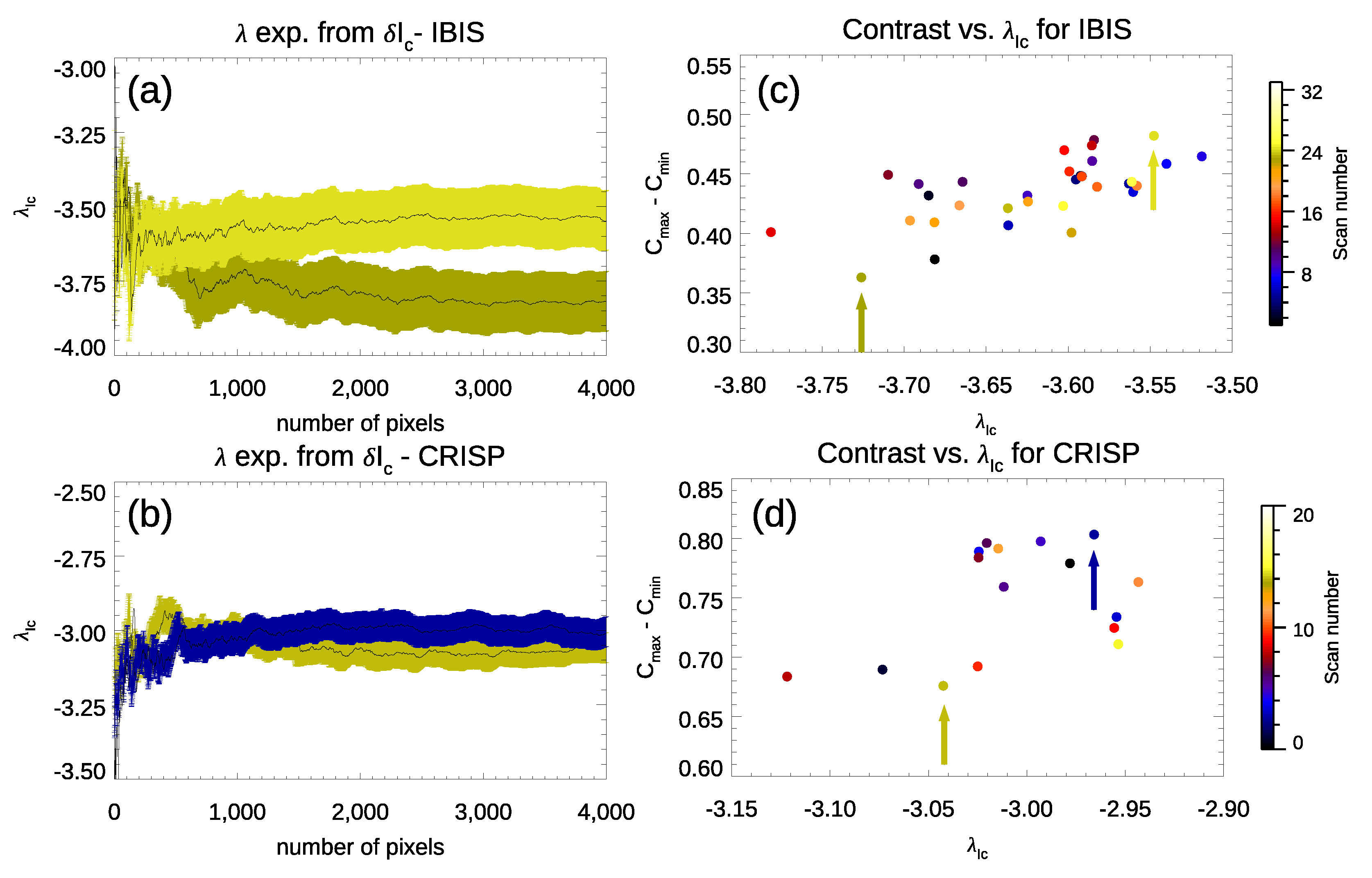
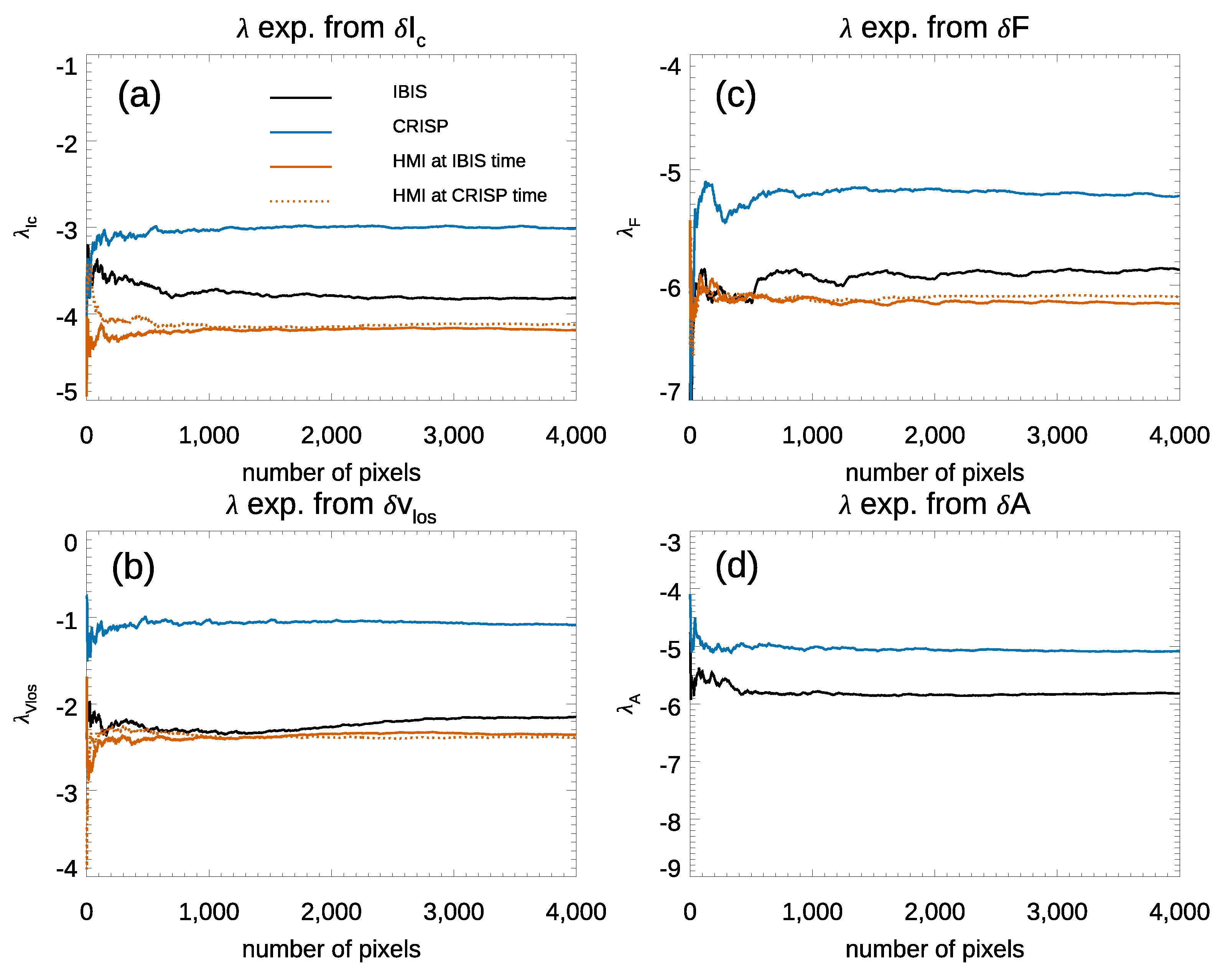
| −3.00 ± 0.05 | −3.6 ± 0.1 | −4.2 ± 1.5 | −4.2 ± 2.0 | |
| −1.02 ± 0.06 | −2.1 ± 0.2 | |||
| −5.18 ± 0.06 | −5.6 ± 0.1 | |||
| −5.12 ± 0.06 | −6.0 ± 0.4 | - | - |
| Kernel 2 × 2 (subgranular) | −3.8 ± 0.1 | −2.2 ± 0.2 | −5.7 ± 0.1 | −6.2 ± 0.4 |
| Kernel 5 × 5 (granular) | −4.3 ± 0.1 | −2.5 ± 0.2 | −5.8 ± 0.1 | −6.5 ± 0.4 |
| Kernel 28 × 28 (mesogranular) | −5.6 ± 0.3 | −3.2 ± 0.3 | −6.2 ± 0.2 | −7.1 ± 0.5 |
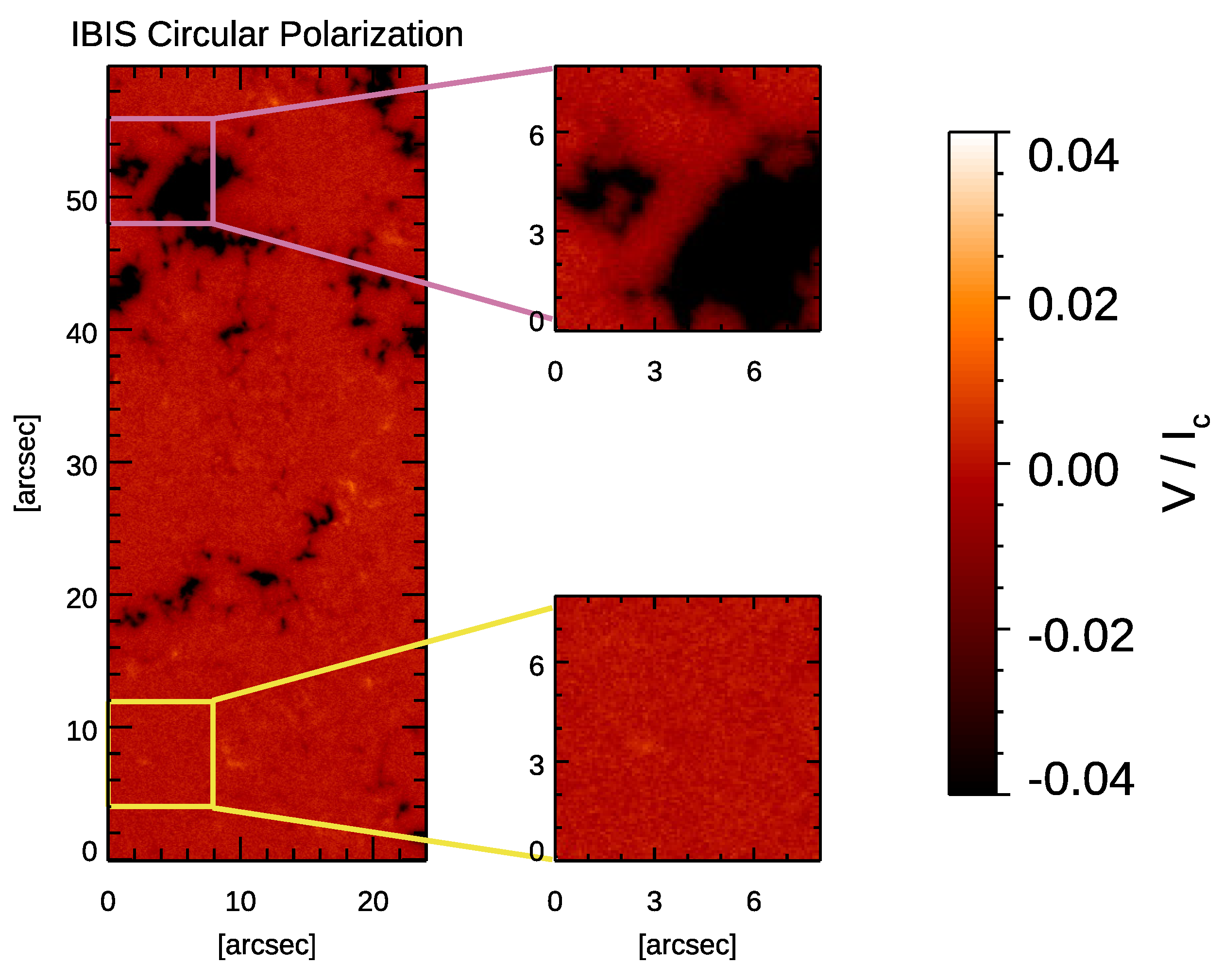
| Magnetic sub-FoV | −3.9 ± 0.2 | −2.1 ± 0.3 | −5.8 ± 0.2 | −5.9 ± 0.4 |
| Quiet sub-FoV | −3.6 ± 0.1 | −2.2 ± 0.3 | −5.8 ± 0.2 | −6.2 ± 0.2 |
Publisher’s Note: MDPI stays neutral with regard to jurisdictional claims in published maps and institutional affiliations. |
© 2021 by the authors. Licensee MDPI, Basel, Switzerland. This article is an open access article distributed under the terms and conditions of the Creative Commons Attribution (CC BY) license (https://creativecommons.org/licenses/by/4.0/).
Share and Cite
Viavattene, G.; Murabito, M.; Guglielmino, S.L.; Ermolli, I.; Consolini, G.; Giorgi, F.; Jafarzadeh, S. Analysis of Pseudo-Lyapunov Exponents of Solar Convection Using State-of-the-Art Observations. Entropy 2021, 23, 413. https://doi.org/10.3390/e23040413
Viavattene G, Murabito M, Guglielmino SL, Ermolli I, Consolini G, Giorgi F, Jafarzadeh S. Analysis of Pseudo-Lyapunov Exponents of Solar Convection Using State-of-the-Art Observations. Entropy. 2021; 23(4):413. https://doi.org/10.3390/e23040413
Chicago/Turabian StyleViavattene, Giorgio, Mariarita Murabito, Salvatore L. Guglielmino, Ilaria Ermolli, Giuseppe Consolini, Fabrizio Giorgi, and Shahin Jafarzadeh. 2021. "Analysis of Pseudo-Lyapunov Exponents of Solar Convection Using State-of-the-Art Observations" Entropy 23, no. 4: 413. https://doi.org/10.3390/e23040413