
A Hybrid Preaching Optimization Algorithm Based on Kapur Entropy for Multilevel Thresholding Color Image Segmentation

Abstract
:1. Introduction
2. POA Algorithm
2.1. Religious Inheritance
2.2. Religious Competition
2.3. Religious Development
3. A Novel HPOA Algorithm
3.1. Evolutionary State Estimation
3.2. Distributed Time-Delay Based on PSO Idea
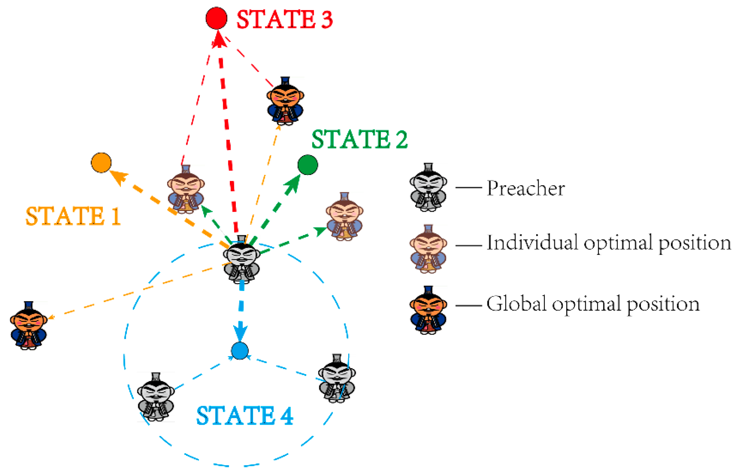
3.3. Adaptive Orientation Adjustment Strategy Based on Evolutionary State
3.3.1. State 1: Exploration
3.3.2. State 2: Exploitation
3.3.3. State 3: Convergence
3.3.4. State 4: Escape
3.4. The Framework of the HPOA
- (1)
- Initialize the parameters including the population size, the max number of iterations, the search dimension, the number of inheritors, and the number of elite individuals.
- (2)
- Initialize the population.
- (3)
- Record global and local optimal historical information.
- (4)
- Transmit the location information to inheritors using Equation (1).
- (5)
- Select new preachers by the mechanism of religion competition using Equation (2).
- (6)
- Estimating the evolutionary state of the new preachers using Equations (4)–(6).
- (7)
- Adding distributed time-delay to the preachers based on their evolutionary state.
- (8)
- Search for a new solution by the mechanism of religion development by Equation (3).
- (9)
- Repeat Steps 3 to 5 till the algorithm meets the max number of iterations.
- (10)
- Output the result.
4. HPOA-Based Segmentation Algorithm
4.1. Multilevel Thresholding Image Segmentation
4.2. Kapur Entropy
4.3. Implementation of the HPOA-Based Segmentation Algorithm
5. Simulation and Discussion of the HPOA Algorithm
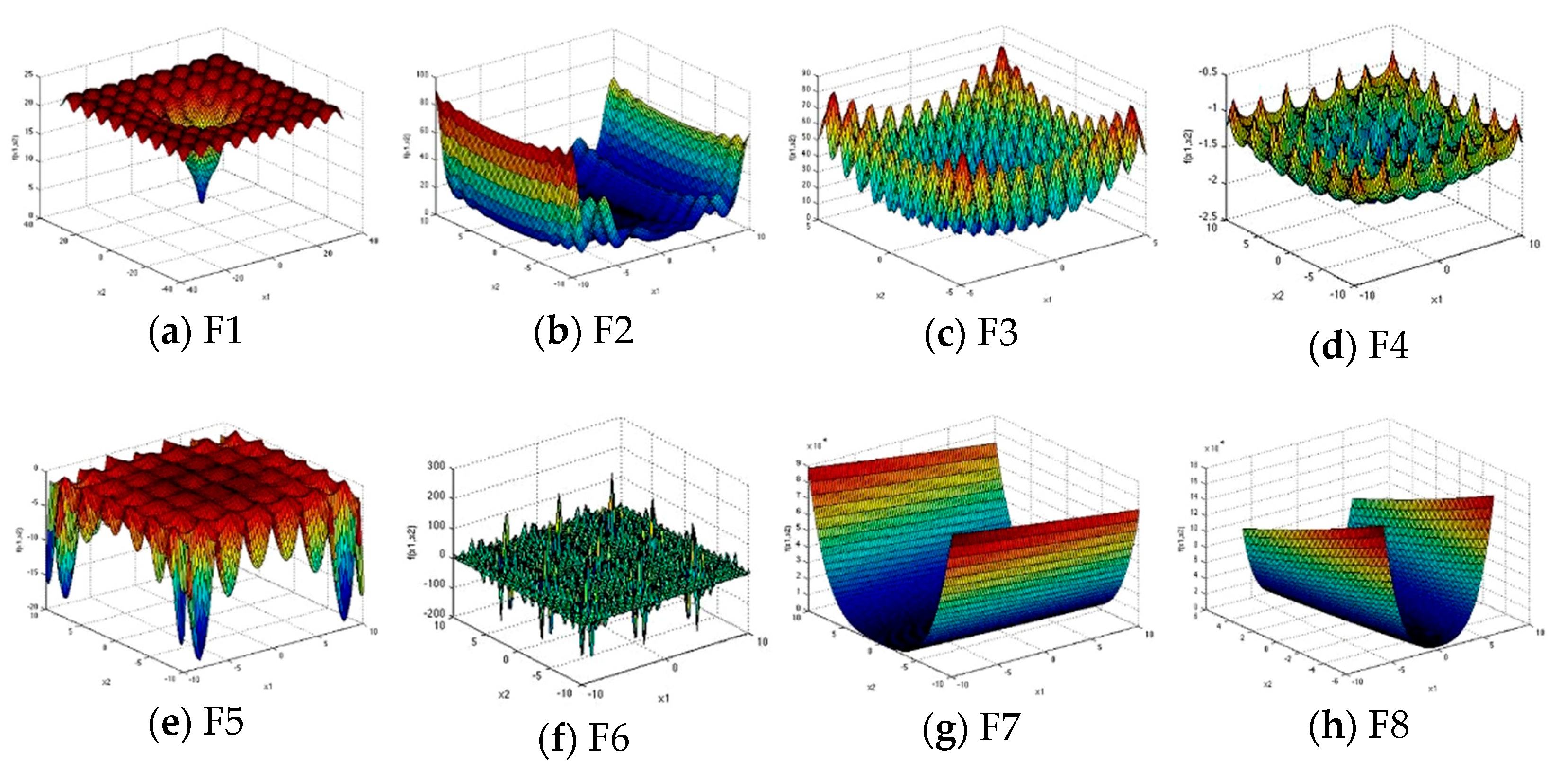
5.1. Selection of Benchmark Functions
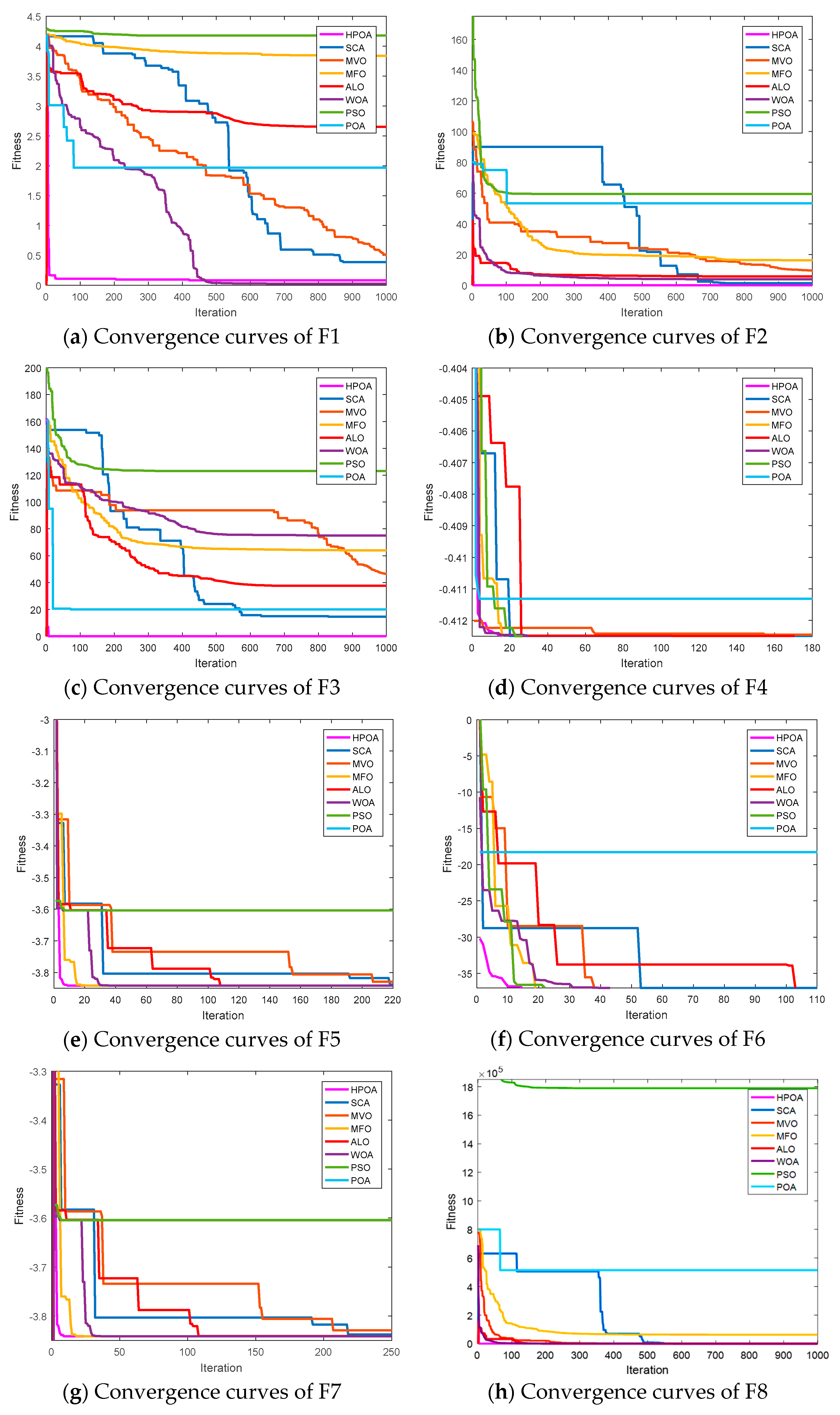
5.2. Experimental Setup
- (1)
- Traditional POA algorithm [32].
- (2)
- The state-of-the-art WOA algorithm, in which is flexible and requires fewer parameters to be adjusted [42].
- (3)
- The classical representative of swarm intelligence: PSO [30].
- (4)
- A newly proposed algorithm named SCA, containing several adaptive variables to ensure a balance between exploration and development [28].
- (5)
- A novel natural heuristic algorithm: MVO, designed for engineering structure design [41].
- (6)
- MFO, inspired by moth navigation which has advantages in solving unknown space problems [40].
- (7)
- An interesting algorithm, ALO, along with characteristics of few adjusting parameters and high accuracy [53].
5.3. Experimental Results of HPOA
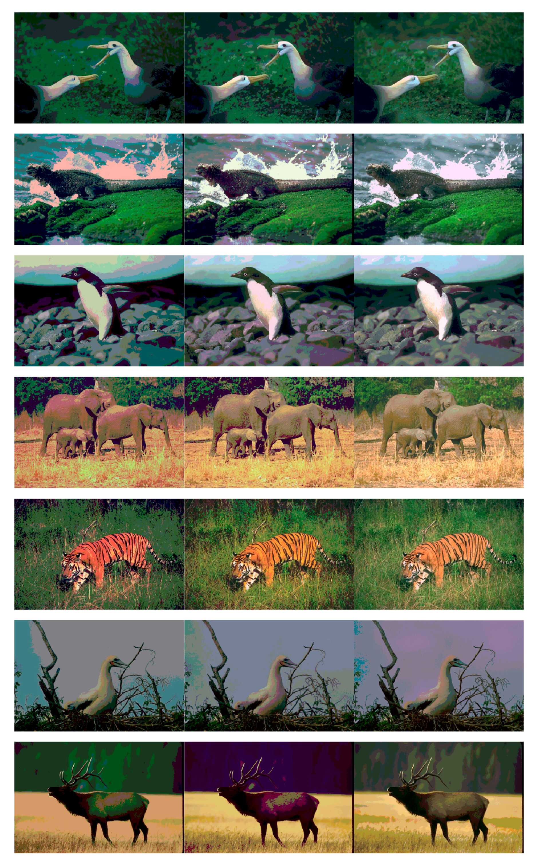
6. Results and Discussion of the HPOA-Based Segmentation Algorithm
6.1. Experimental Setup
6.2. Image Evaluation Metric
6.2.1. Feature Similarity Index (FSIM)
6.2.2. Peak Signal to Noise Ratio (PSNR)
6.2.3. Structural Similarity Index (SSIM)
6.3. Experimental Result
7. Conclusions
Author Contributions
Funding
Institutional Review Board Statement
Informed Consent Statement
Data Availability Statement
Conflicts of Interest
References
- He, K.; Gkioxari, G.; Dollar, P.; Girshick, R. Mask R-CNN. IEEE Trans. Pattern Anal. Mach. Intell. 2020, 42, 386–397. [Google Scholar] [CrossRef] [PubMed]
- Bhandari, A.K. A novel beta differential evolution algorithm-based fast multilevel thresholding for color image segmentation. Neural Comput. Appl. 2020, 32, 4583–4613. [Google Scholar] [CrossRef]
- Li, K.; Qi, X.; Luo, Y.; Yao, Z.; Sun, M. Accurate retinal vessel segmentation in color fundus images via fully attention-based networks. IEEE J. Biomed. Health 2021, 25, 2071–2081. [Google Scholar] [CrossRef]
- Farhat, W.; Sghaier, H.; Faiedh, H.; Souani, C. Design of efficient embedded system for road sign recognition. J. Ambient Intell. Humaniz. Comput. 2019, 10, 491–507. [Google Scholar] [CrossRef]
- Gao, G.; Xiao, K.; Jia, Y. A spraying path planning algorithm based on colour-depth fusion segmentation in peach orchards. Comput. Electron. Agric. 2020, 173, 105412. [Google Scholar] [CrossRef]
- Zhao, D.; Liu, L.; Yu, F.; Heidari, A.A.; Wang, M.; Oliva, D.; Muhammad, K.; Chen, H. Ant colony optimization with horizontal and vertical crossover search: Fundamental visions for multi-threshold image segmentation. Expert Syst. Appl. 2020, 167, 114122. [Google Scholar] [CrossRef]
- He, C.; Li, S.; Xiong, D.; Fang, P.; Liao, M. Remote sensing image semantic segmentation based on edge information guidance. Remote Sens. 2020, 12, 1501. [Google Scholar] [CrossRef]
- Shao, Z.; Zhou, W.; Deng, X.; Zhang, M.; Cheng, Q. Multilabel Remote Sensing Image Retrieval Based on Fully Convolutional Network. IEEE J. Sel. Top. Appl. Earth Observ. Remote Sens. 2020, 13, 318–328. [Google Scholar] [CrossRef]
- Keuper, M.; Tang, S.; Andres, B.; Brox, T.; Schiele, B. Motion Segmentation & Multiple Object Tracking by Correlation Co-Clustering. IEEE T. Pattern Anal. 2020, 42, 140–153. [Google Scholar]
- Levinshtein, A.; Stere, A.; Kutulakos, K.N.; Fleet, D.J.; Dickinson, S.J.; Siddiqi, K. Turbopixels: Fast superpixels using geometric flows. IEEE Trans. Pattern Anal. Mach. Intell. 2009, 31, 2290–2297. [Google Scholar]
- Stutz, D.; Hermans, A.; Leibe, B. Superpixels: An evaluation of the state-of-the-art. Comput. Vis. Image Underst. 2018, 166, 1–27. [Google Scholar] [CrossRef] [Green Version]
- Ciecholewski, M. Automated coronal hole segmentation from Solar EUV Images using the watershed transform. J. Vis. Commun. Image Represent. 2015, 33, 203–218. [Google Scholar] [CrossRef]
- Cousty, J.; Bertrand, G.; Najman, L.; Couprie, M. Watershed cuts: Thinnings, shortest path forests, and topological watersheds. IEEE Trans. Pattern Anal. Mach. Intell. 2010, 32, 925–939. [Google Scholar] [CrossRef] [PubMed] [Green Version]
- Zhao, L.; Gao, X.; Yuan, Y.; Tao, D. Geometric active curve for selective entropy optimization. Neurocomputing 2014, 139, 65–76. [Google Scholar]
- Ding, K.; Xiao, L.; Weng, G. Active contours driven by region-scalable fitting and optimized Laplacian of Gaussian energy for image segmentation. Signal Process. 2017, 134, 224–233. [Google Scholar] [CrossRef]
- Zhou, Z.; Siddiquee, M.M.R.; Tajbakhsh, N.; Liang, J. UNet plus plus: Redesigning skip connections to exploit multiscale features in image segmentation. IEEE T. Med. Imaging 2020, 42, 140–153. [Google Scholar]
- Breve, F. Interactive image segmentation using label propagation through complex networks. Expert Syst. Appl. 2019, 123, 18–33. [Google Scholar] [CrossRef] [Green Version]
- Lang, C.; Jia, H. Kapur’s Entropy for Color Image Segmentation Based on a Hybrid Whale Optimization Algorithm. Entropy 2019, 123, 318. [Google Scholar] [CrossRef] [Green Version]
- Bhandari, A.K.; Singh, A.; Kumar, I.V. Spatial Context Energy Curve-Based Multilevel 3-D Otsu Algorithm for Image Segmentation. IEEE Trans. Syst. Man Cybern.-Syst. 2021, 51, 2760–2773. [Google Scholar] [CrossRef]
- Back, A.D.; Angus, D.; Wiles, J. Transitive entropy-a rank ordered approach for natural sequences. IEEE J. Sel. Top. Signal Process. 2020, 14, 312–321. [Google Scholar] [CrossRef]
- Wu, C.; Cao, Z. Entropy-like divergence based kernel fuzzy clustering for robust image segmentation. Expert Syst. Appl. 2021, 169, 114327. [Google Scholar] [CrossRef]
- Rahaman, J.; Sing, M. An efficient multilevel thresholding based satellite image segmentation approach using a new adaptive cuckoo search algorithm. Expert Syst. Appl. 2021, 174, 114633. [Google Scholar] [CrossRef]
- Jalab, H.A.; Al-Shamasneh, A.R.; Shaiba, H.; Ibrahim, R.W.; Baleanu, D. Fractional renyi entropy image enhancement for deep segmentation of kidney mri. CMC-Comput. Mater. Con. 2021, 67, 2061–2075. [Google Scholar]
- Zhao, D.; Liu, L.; Yu, F.; Heidari, A.A.; Chen, H. Chaotic random spare ant colony optimization for multi-threshold image segmentation of 2D Kapur entropy. Knowl.-Based Syst. 2021, 216, 106510. [Google Scholar] [CrossRef]
- Rodriguez-Esparza, E.; Zanella-Calzada, L.A.; Oliva, D.; Heidari, A.A.; Foong, L.K. An efficient Harris hawks-inspired image segmentation method. Expert Syst. Appl. 2020, 155, 113428. [Google Scholar] [CrossRef]
- Abdel-Basset, M.; Mohamed, R.; Elhoseny, M.; Chakrabortty, R.K.; Ryan, M. A hybrid covid-19 detection model using an improved marine predators algorithm and a ranking-based diversity reduction strategy. IEEE Access 2020, 8, 79521–79540. [Google Scholar] [CrossRef]
- Upadhyay, P.; Chhabra, J.K. Kapur’s entropy based optimal multilevel image segmentation using crow search algorithm. Appl. Soft. Comput. 2019, 1, 105522. [Google Scholar] [CrossRef]
- Gupta, S.; Deep, K. Improved sine cosine algorithm with crossover scheme for global optimization. Knowl.-Based Syst. 2019, 165, 374–406. [Google Scholar] [CrossRef]
- Xue, J.; Shen, B. A novel swarm intelligence optimization approach: Sparrow search algorithm. Syst. Sci. Control Eng. 2020, 8, 22–34. [Google Scholar] [CrossRef]
- Martino, F.D.; Sessa, S. PSO image thresholding on images compressed via fuzzy transforms. Inform. Sciences 2020, 506, 308–324. [Google Scholar] [CrossRef]
- Jia, H.; Peng, X.; Song, W.; Lang, C.; Xing, Z.; Sun, K. Multiverse optimization algorithm based on levy flight improvement for multithreshold color image segmentation. IEEE Access 2019, 7, 32805–32844. [Google Scholar] [CrossRef]
- Wei, D.; Wang, Z.; Si, L.; Tan, C. Preaching-inspired swarm intelligence algorithm and its applications. Knowl.-Based Syst. 2021, 211, 106552. [Google Scholar] [CrossRef]
- Mirjalili, S.; Gandomi, A.H.; Mirjalili, S.Z.; Saremi, S.; Faris, H.; Mirjalili, S.M. Salp swarm algorithm: A bio-inspired optimizer for engineering design problems. Adv. Eng. Softw. 2017, 114, 163–191. [Google Scholar] [CrossRef]
- Mirjalili, S.M.; Mirjalili, S.; Lewis, A. Grey wolf optimizer. Adv. Eng. Softw. 2014, 69, 46–61. [Google Scholar] [CrossRef] [Green Version]
- Baniani, E.A.; Chalechale, A. Hybrid pso and genetic algorithm for multilevel maximum entropy criterion threshold selection. Int. J. Hydrog. Energy 2013, 6, 131–140. [Google Scholar] [CrossRef]
- Liu, Z.; Wei, H.; Zhong, Q.; Liu, K.; Xiao, X.; Wu, L. Parameter estimation for VSI-Fed PMSM based on a dynamic PSO with learning strategies. IEEE T. Power Electr. 2017, 32, 3154–3165. [Google Scholar] [CrossRef] [Green Version]
- Yang, X. Firefly algorithms for multimodal optimization. In Proceedings of the 5th International Conference on Stochastic Algorithms: Foundations and Applications, Sapporo, Japan, 26–28 October 2009; Volume 5792, pp. 169–178. [Google Scholar]
- Xu, J.; Wang, Z.; Tan, C.; Si, L.; Liu, X. Cutting pattern identification for coal mining shearer through a swarm intelligence-based variable translation wavelet neural network. Sensors 2018, 18, 382. [Google Scholar] [CrossRef] [Green Version]
- Heidari, A.A.; Mirjalili, S.; Faris, H.; Aljarah, I.; Mafarja, M.; Chen, H. Harris hawks optimization: Algorithm and applications. Futur. Gener. Comp. Syst. 2019, 97, 849–872. [Google Scholar] [CrossRef]
- Mirjalili, S. Moth-flame optimization algorithm: A novel nature-inspired heuristic paradigm. Knowl.-Based Syst. 2015, 89, 228–249. [Google Scholar] [CrossRef]
- Mirjalili, S.; Mirjalili, S.M.; Hatamlou, A. Multi-verse optimizer: A nature-inspired algorithm for global optimization. Neural Comput. Appl. 2016, 27, 495–513. [Google Scholar] [CrossRef]
- Mirjalili, S.; Lewis, A. The whale optimization algorithm. Adv. Eng. Softw. 2016, 95, 51–67. [Google Scholar] [CrossRef]
- Wolpert, D.H.; Macready, W.G. No free lunch theorems for optimization. IEEE Trans. Evol. Comput. 1997, 1, 67–82. [Google Scholar] [CrossRef] [Green Version]
- Song, B.; Wang, Z.; Zou, L. On global smooth path planning for mobile robots using a novel multimodal delayed PSO algorithm. Cogn. Comput. 2017, 9, 5–17. [Google Scholar] [CrossRef]
- Tang, Y.; Wang, Z.; Fang, J. Parameters identification of unknown delayed genetic regulatory networks by a switching particle swarm optimization algorithm. Expert Syst. Appl. 2011, 38, 2523–2535. [Google Scholar] [CrossRef] [Green Version]
- Zeng, N.; Wang, Z.; Zhang, H.; Alsaadi, F.E. A novel switching delayed pso algorithm for estimating unknown parameters of lateral flow immunoassay. Cogn. Comput. 2016, 8, 143–152. [Google Scholar]
- Song, Q.; Wang, Z. Neural networks with discrete and distributed time-varying delays: A general stability analysis. Chaos Soliton. Fract. 2008, 37, 1538–1547. [Google Scholar] [CrossRef]
- Liu, W.; Wang, Z.; Liu, X.; Zeng, N.; Bell, D. A novel particle swarm optimization approach for patient clustering from emergency departments. IEEE Trans. Evol. Comput. 2019, 23, 632–644. [Google Scholar] [CrossRef] [Green Version]
- Zhan, Z.; Zhang, J.; Li, Y.; Chung, H.S.H. Adaptive particle swarm optimization. IEEE Trans. Syst. Man Cybern. Part B-Cybern. 2009, 39, 1362–1381. [Google Scholar] [CrossRef] [Green Version]
- Bergh, F.; Engelbrecht, A.P. A study of particle swarm optimization particle trajectories. Inform. Sci. 2005, 176, 937–971. [Google Scholar]
- Liu, X.; Zhan, Z.; Gao, Y.; Zhang, J.; Kwong, S.; Zhang, J. Coevolutionary particle swarm optimization with bottleneck objective learning strategy for many-objective optimization. IEEE Trans. Evol. Comput. 2019, 23, 587–602. [Google Scholar] [CrossRef]
- Yao, X.; Liu, Y.; Lin, G. Evolutionary programming made faster. IEEE Trans. Evol. Comput. 1999, 3, 82–102. [Google Scholar]
- Mirjalili, S. The ant lion optimizer. Adv. Eng. Softw. 2015, 83, 80–98. [Google Scholar] [CrossRef]
- Zhang, L.; Zhang, L.; Mou, X.; Zhang, D. Fsim: A feature similarity index for image quality assessment. IEEE Trans. Image Process. 2011, 20, 2378–2386. [Google Scholar] [CrossRef] [PubMed] [Green Version]
- Huynh-Thu, Q.; Ghanbari, M. Scope of validity of PSNR in image/video quality assessment. Electron. Lett. 2008, 44, 800–835. [Google Scholar] [CrossRef]
- He, L.; Huang, S. Modified firefly algorithm based multilevel thresholding for color image segmentation. Neurocomputing 2017, 240, 152–174. [Google Scholar] [CrossRef]
- Aziz, M.A.E.; Ewees, A.A.; Hassanien, A.E. Whale Optimization Algorithm and Moth-Flame Optimization for multilevel thresholding image segmentation. Expert Syst. Appl. 2017, 83, 242–256. [Google Scholar] [CrossRef]
- Wang, Z.; Bovik, A.C.; Sheikh, H.R.; Simoncelli, E.P. Image quality assessment: From error visibility to structural similarity. IEEE Trans. Image Process. 2004, 13, 600–612. [Google Scholar] [CrossRef] [Green Version]
- Arbelaez, P.; Maire, M.; Fowlkes, C.; Malik, J. Contour Detection and Hierarchical Image Segmentation. IEEE Trans. Pattern Anal. Mach. Intell. 2010, 33, 898–916. [Google Scholar] [CrossRef] [Green Version]
- Bandyopadhyay, R.; Kundu, R.; Oliva, D.; Sarkar, R. Segmentation of brain MRI using an altruistic Harris Hawks’ Optimization algorithm. Knowl.-Based Syst. 2021, 232, 107468. [Google Scholar] [CrossRef]
- Zeng, N.; Zhang, H.; Song, B.; Liu, W.; Li, Y.; Dobaie, A.M. Facial expression recognition via learning deep sparse autoencoders. Neurocomputing 2018, 273, 643–649. [Google Scholar] [CrossRef]
- Gandomi, A.H.; Yang, X.; Alavi, A.H. Cuckoo search algorithm: A metaheuristic approach to solve structural optimization problems. Eng. Comput. 2013, 1, 17–35. [Google Scholar] [CrossRef]
- Faramarzi, A.; Heidarinejad, M.; Mirjalili, S.; Gandomi, A.H. Marine Predators Algorithm: A nature-inspired metaheuristic. Expert Syst. Appl. 2020, 152, 113377. [Google Scholar] [CrossRef]


| Functions | Name | Dimension | Search Space |
|---|---|---|---|
| F1 | Ackley Function | d | [−32.768, 32.768] |
| F2 | Levy Function | d | [−10, 10] |
| F3 | Rastrigin Function | d | [−5.12, 5.12] |
| F4 | Cross-in-Tray Function | 2 | [−10, 10] |
| F5 | Holder Table Function | 2 | [−10, 10] |
| F6 | Shubert Function | 2 | [−5.12, 5.12] |
| F7 | Dixon-Price Function | d | [−10, 10] |
| F8 | Rosenbrock Function | d | [−5, 10] |
| Functions | HPOA (N = 25) | HPOA (N = 50) | HPOA (N = 75) | HPOA (N = 100) | HPOA (N = 125) | HPOA (N = 150) | HPOA (N = 175) | HPOA (N = 200) |
|---|---|---|---|---|---|---|---|---|
| F1 | 0.52495 | 0.32073 | 0.30325 | 0.36599 | 0.33331 | 0.50970 | 0.39105 | 0.24924 |
| F2 | 0.02400 | 0.02138 | 0.02263 | 0.02193 | 0.02115 | 0.01104 | 0.01482 | 0.01894 |
| F3 | 0.00022 | 0.00870 | 0.00002 | 0.00000 | 0.00000 | 0.00000 | 0.00000 | 0.00000 |
| F4 | −2.06261 | −2.06261 | −2.06261 | −2.06261 | −2.06261 | −2.06261 | −2.06261 | −2.06261 |
| F5 | −19.20828 | −19.20850 | −19.20850 | −19.20850 | −19.20850 | −19.20850 | −19.20850 | −19.20850 |
| F6 | −186.73068 | −186.73083 | −186.73032 | −186.73089 | −186.73090 | −186.73090 | −186.73068 | −186.73088 |
| F7 | 0.40187 | 0.86632 | 0.32475 | 0.66930 | 0.47461 | 0.54274 | 0.39958 | 0.62513 |
| F8 | 4.32519 | 0.00000 | 0.00000 | 0.00000 | 3.45213 | 4.67038 | 3.22098 | 4.85049 |
| Functions | HPOA (N = 25) | HPOA (N = 50) | HPOA (N = 75) | HPOA (N = 100) | HPOA (N = 125) | HPOA (N = 150) | HPOA (N = 175) | HPOA (N = 200) |
|---|---|---|---|---|---|---|---|---|
| F1 | 0.382 | 0.223 | 0.239 | 0.168 | 0.234 | 0.519 | 0.235 | 0.277 |
| F2 | 0.02537 | 0.02506 | 0.02657 | 0.02342 | 0.02331 | 0.01878 | 0.02088 | 0.02141 |
| F3 | 0.00055 | 0.02733 | 2.51 × 10⁻⁵ | 3.68 × 10⁻⁶ | 1.62 × 10⁻⁷ | 2.84 × 10⁻⁶ | 1.27 × 10⁻⁷ | 5.94 × 10⁻⁷ |
| F4 | 7.95 × 10⁻¹¹ | 3.49 × 10⁻¹¹ | 9.26 × 10⁻¹⁰ | 9.82 × 10⁻¹⁰ | 7.64 × 10⁻¹¹ | 5.05 × 10⁻¹¹ | 1.31 × 10⁻⁹ | 2.43 × 10⁻¹⁰ |
| F5 | 0.00070 | 4.43 × 10⁻⁸ | 3.28 × 10⁻⁷ | 4.60 × 10⁻⁷ | 4.14 × 10⁻⁷ | 7.69 × 10⁻⁷ | 1.12 × 10⁻⁶ | 6.78 × 10⁻⁷ |
| F6 | 0.00036 | 0.00023 | 0.00182 | 1.89 × 10⁻⁵ | 1.99 × 10⁻⁵ | 1.32 × 10⁻⁵ | 0.00056 | 7.41 × 10⁻⁵ |
| F7 | 0.315 | 0.971 | 0.237 | 0.859 | 0.362 | 0.379 | 0.316 | 0.394 |
| F8 | 13.6 | 9.05 × 10⁻⁷ | 4.91 × 10⁻⁶ | 1.03 × 10⁻⁶ | 10.9 | 14.8 | 10.2 | 15.3 |
| Functions | HPOA (N = 25) | HPOA (N = 50) | HPOA (N = 75) | HPOA (N = 100) | HPOA (N = 125) | HPOA (N = 150) | HPOA (N = 175) | HPOA (N = 200) |
|---|---|---|---|---|---|---|---|---|
| F1 | 0.24924 | 1.41404 | 4.16335 | 18.83677 | 13.55022 | 1.51994 | 20.97066 | 8.86645 |
| F2 | 0.01894 | 19.21614 | 53.66761 | 76.44632 | 21.69743 | 20.91945 | 366.39623 | 288.52300 |
| F3 | 3.46 × 10⁻⁷ | 73.46613 | 224.93067 | 377.08160 | 154.82146 | 229.48096 | 624.51340 | 145.85033 |
| F4 | −2.06261 | −2.06260 | −2.06261 | −2.06261 | −2.06261 | −2.06261 | −2.06261 | −2.04456 |
| F5 | −19.20850 | −19.17267 | −19.20850 | −19.08972 | −19.20850 | −19.20850 | −17.96997 | −10.38813 |
| F6 | −186.73088 | −186.50028 | −175.99883 | −186.73091 | −186.73091 | −186.73091 | −186.73091 | −65.73965 |
| F7 | 0.625 | 1.28 × 10⁴ | 25.3 | 3.26 × 10⁵ | 16.7 | 8.45 | 6.63 × 10⁶ | 4.95 × 10⁶ |
| F8 | 4.85049 | 2512.80140 | 80.14614 | 392,657.86 | 130.60844 | 57.3 | 6.59 × 10⁶ | 3.33 × 10⁶ |
| Functions | HPOA (N = 25) | HPOA (N = 50) | HPOA (N = 75) | HPOA (N = 100) | HPOA (N = 125) | HPOA (N = 150) | HPOA (N = 175) | HPOA (N = 200) |
|---|---|---|---|---|---|---|---|---|
| F1 | 0.277 | 1.42 | 5.46 | 1.07 | 3.49 | 1.39 | 0.126 | 1.65 |
| F2 | 0.02 | 14.24 | 15.49 | 28.14 | 7.03 | 14.08 | 91.95 | 15.54 |
| F3 | 0.00 | 32.03 | 31.65 | 71.59 | 27.15 | 101.15 | 53.60 | 53.04 |
| F4 | 2.43 × 10⁻¹⁰ | 1.99 × 10⁻⁵ | 6.83 × 10⁻⁹ | 4.68 × 10⁻¹⁶ | 6.34 × 10⁻¹⁵ | 3.99 × 10⁻¹⁵ | 4.68 × 10⁻¹⁶ | 0.04 |
| F5 | 6.78 × 10⁻⁷ | 0.03 | 1.45 × 10⁻⁶ | 0.38 | 4.53 × 10⁻¹³ | 8.22 × 10⁻¹⁴ | 1.28 | 3.77 |
| F6 | 7.41 × 10⁻⁵ | 0.327 | 33.94 | 1.64 × 10⁻¹⁴ | 4.88 × 10⁻¹¹ | 1.24 × 10⁻¹³ | 0.00 | 29.97 |
| F7 | 0.394 | 1.39 × 10⁴ | 23.7 | 4.58 × 10⁵ | 10.3 | 8.50 | 3.15 × 10⁶ | 6.72 × 10⁵ |
| F8 | 15.3 | 2.43 × 10³ | 50.23 | 272,823.47 | 74.38 | 14.51 | 1.76 × 10⁶ | 484,632.28 |
| Functions | HPOA vs. SCA | HPOA vs. MVO | HPOA vs. MFO | HPOA vs. ALO | HPOA vs. WOA | HPOA vs. PSO | HPOA vs. POA | |||||||
|---|---|---|---|---|---|---|---|---|---|---|---|---|---|---|
| p-Valve | h | p-Valve | h | p-Valve | h | p-Valve | h | p-Valve | h | p-Valve | h | p-Valve | h | |
| F1 | 0.037635 | 1 | 0.000183 | 1 | 0.000183 | 1 | 0.000183 | 1 | 0.011330 | 1 | 0.000183 | 1 | 0.000183 | 1 |
| F2 | 0.000183 | 1 | 0.000183 | 1 | 0.000183 | 1 | 0.000183 | 1 | 0.000183 | 1 | 0.000183 | 1 | 0.000183 | 1 |
| F3 | 0.000183 | 1 | 0.000183 | 1 | 0.000183 | 1 | 0.000183 | 1 | 0.000183 | 1 | 0.000183 | 1 | 0.000183 | 1 |
| F4 | 0.000183 | 1 | 0.000246 | 1 | 0.000064 | 1 | 0.000504 | 1 | 0.000242 | 1 | 0.000064 | 1 | 0.000183 | 1 |
| F5 | 0.000183 | 1 | 0.121225 | 0 | 0.002036 | 1 | 0.000183 | 1 | 0.000173 | 1 | 0.471171 | 0 | 0.000183 | 1 |
| F6 | 0.000183 | 1 | 0.004586 | 1 | 0.000129 | 1 | 0.000769 | 1 | 0.000173 | 1 | 0.000141 | 1 | 0.000183 | 1 |
| F7 | 0.000183 | 1 | 0.000183 | 1 | 0.000183 | 1 | 0.000183 | 1 | 0.000183 | 1 | 0.000183 | 1 | 0.000183 | 1 |
| Original Image | Histogram | Original Image | Histogram |
|---|---|---|---|
| Animal | |||
 |  |  |  |
| (a) P1-1 | (b) P1-2 | ||
 |  |  |  |
| (c) P1-3 | (d) P1-4 | ||
 |  |  |  |
| (e) P1-5 | (f) P1-6 | ||
 |  |  |  |
| (g) P1-7 | (h) P1-8 | ||
| Human | |||
 |  |  |  |
| (i) P2-1 | (j) P2-2 | ||
 |  |  |  |
| (k) P2-3 | (l) P2-4 | ||
 |  |  |  |
| (m) P2-5 | (n) P2-6 | ||
 |  |  |  |
| (o) P2-7 | (p) P2-8 | ||
| Architecture | |||
 |  |  |  |
| (q) P3-1 | (r) P3-2 | ||
 |  |  |  |
| (s) P3-3 | (t) P3-4 | ||
 |  |  |  |
| (u) P3-5 | (v) P3-6 | ||
 |  |  |  |
| (w) P3-7 | (x) P3-8 | ||
| Image | Dim | HPOA | SCA | MVO | MFO | ALO | WOA | PSO | POA |
|---|---|---|---|---|---|---|---|---|---|
| P1-1 | 5 | 0.40 | 0.37 | 0.38 | 0.38 | 0.38 | 0.37 | 0.38 | 0.35 |
| 10 | 0.47 | 0.46 | 0.43 | 0.42 | 0.43 | 0.43 | 0.42 | 0.44 | |
| 15 | 0.43 | 0.43 | 0.41 | 0.42 | 0.42 | 0.41 | 0.42 | 0.39 | |
| P1-2 | 5 | 0.50 | 0.47 | 0.49 | 0.50 | 0.49 | 0.48 | 0.48 | 0.37 |
| 10 | 0.55 | 0.52 | 0.53 | 0.53 | 0.52 | 0.52 | 0.53 | 0.50 | |
| 15 | 0.48 | 0.42 | 0.46 | 0.48 | 0.40 | 0.42 | 0.47 | 0.43 | |
| P1-3 | 5 | 0.56 | 0.42 | 0.54 | 0.52 | 0.51 | 0.51 | 0.50 | 0.56 |
| 10 | 0.58 | 0.47 | 0.54 | 0.54 | 0.55 | 0.51 | 0.56 | 0.53 | |
| 15 | 0.56 | 0.48 | 0.50 | 0.54 | 0.55 | 0.48 | 0.49 | 0.51 | |
| P1-4 | 5 | 0.48 | 0.47 | 0.46 | 0.44 | 0.46 | 0.41 | 0.42 | 0.42 |
| 10 | 0.47 | 0.41 | 0.43 | 0.44 | 0.41 | 0.46 | 0.47 | 0.46 | |
| 15 | 0.53 | 0.52 | 0.50 | 0.52 | 0.48 | 0.50 | 0.50 | 0.49 | |
| P1-5 | 5 | 0.48 | 0.47 | 0.46 | 0.46 | 0.41 | 0.46 | 0.42 | 0.46 |
| 10 | 0.50 | 0.47 | 0.42 | 0.48 | 0.41 | 0.45 | 0.43 | 0.40 | |
| 15 | 0.44 | 0.40 | 0.42 | 0.41 | 0.43 | 0.41 | 0.42 | 0.44 | |
| P1-6 | 5 | 0.49 | 0.47 | 0.43 | 0.45 | 0.48 | 0.48 | 0.47 | 0.40 |
| 10 | 0.55 | 0.53 | 0.55 | 0.53 | 0.52 | 0.54 | 0.54 | 0.54 | |
| 15 | 0.60 | 0.60 | 0.55 | 0.57 | 0.57 | 0.60 | 0.53 | 0.54 | |
| P1-7 | 5 | 0.47 | 0.41 | 0.45 | 0.44 | 0.44 | 0.41 | 0.44 | 0.42 |
| 10 | 0.55 | 0.51 | 0.52 | 0.54 | 0.50 | 0.52 | 0.55 | 0.55 | |
| 15 | 0.61 | 0.60 | 0.55 | 0.55 | 0.55 | 0.59 | 0.60 | 0.60 | |
| P1-8 | 5 | 0.45 | 0.41 | 0.40 | 0.41 | 0.44 | 0.45 | 0.42 | 0.45 |
| 10 | 0.56 | 0.54 | 0.56 | 0.56 | 0.56 | 0.56 | 0.55 | 0.50 | |
| 15 | 0.61 | 0.54 | 0.60 | 0.56 | 0.55 | 0.59 | 0.60 | 0.58 | |
| P2-1 | 5 | 0.46 | 0.44 | 0.46 | 0.43 | 0.42 | 0.41 | 0.46 | 0.45 |
| 10 | 0.58 | 0.55 | 0.57 | 0.51 | 0.58 | 0.56 | 0.51 | 0.54 | |
| 15 | 0.59 | 0.56 | 0.55 | 0.58 | 0.55 | 0.53 | 0.59 | 0.55 | |
| P2-2 | 5 | 0.57 | 0.42 | 0.55 | 0.54 | 0.51 | 0.57 | 0.50 | 0.50 |
| 10 | 0.58 | 0.50 | 0.53 | 0.54 | 0.58 | 0.56 | 0.55 | 0.53 | |
| 15 | 0.61 | 0.60 | 0.58 | 0.61 | 0.59 | 0.56 | 0.57 | 0.54 | |
| P2-3 | 5 | 0.54 | 0.42 | 0.54 | 0.52 | 0.51 | 0.53 | 0.52 | 0.54 |
| 10 | 0.55 | 0.52 | 0.55 | 0.56 | 0.56 | 0.53 | 0.51 | 0.52 | |
| 15 | 0.62 | 0.60 | 0.56 | 0.57 | 0.55 | 0.54 | 0.54 | 0.59 | |
| P2-4 | 5 | 0.56 | 0.55 | 0.49 | 0.50 | 0.49 | 0.50 | 0.48 | 0.55 |
| 10 | 0.58 | 0.52 | 0.53 | 0.51 | 0.50 | 0.57 | 0.51 | 0.51 | |
| 15 | 0.61 | 0.57 | 0.61 | 0.60 | 0.59 | 0.60 | 0.58 | 0.60 | |
| P2-5 | 5 | 0.49 | 0.43 | 0.44 | 0.42 | 0.40 | 0.47 | 0.42 | 0.42 |
| 10 | 0.58 | 0.52 | 0.51 | 0.56 | 0.51 | 0.57 | 0.55 | 0.51 | |
| 15 | 0.63 | 0.57 | 0.56 | 0.61 | 0.54 | 0.60 | 0.55 | 0.54 | |
| P2-6 | 5 | 0.46 | 0.46 | 0.42 | 0.45 | 0.46 | 0.45 | 0.45 | 0.40 |
| 10 | 0.57 | 0.58 | 0.58 | 0.57 | 0.56 | 0.51 | 0.55 | 0.53 | |
| 15 | 0.62 | 0.60 | 0.55 | 0.59 | 0.58 | 0.61 | 0.60 | 0.59 | |
| P2-7 | 5 | 0.49 | 0.41 | 0.47 | 0.44 | 0.45 | 0.44 | 0.47 | 0.46 |
| 10 | 0.59 | 0.55 | 0.51 | 0.58 | 0.57 | 0.51 | 0.53 | 0.54 | |
| 15 | 0.62 | 0.59 | 0.61 | 0.55 | 0.60 | 0.58 | 0.55 | 0.55 | |
| P2-8 | 5 | 0.49 | 0.46 | 0.42 | 0.47 | 0.43 | 0.47 | 0.41 | 0.43 |
| 10 | 0.58 | 0.57 | 0.58 | 0.57 | 0.56 | 0.51 | 0.53 | 0.54 | |
| 15 | 0.61 | 0.58 | 0.61 | 0.54 | 0.57 | 0.59 | 0.60 | 0.57 | |
| P3-1 | 5 | 0.49 | 0.42 | 0.44 | 0.42 | 0.46 | 0.46 | 0.42 | 0.47 |
| 10 | 0.57 | 0.51 | 0.50 | 0.54 | 0.50 | 0.57 | 0.50 | 0.52 | |
| 15 | 0.61 | 0.61 | 0.58 | 0.54 | 0.61 | 0.57 | 0.60 | 0.61 | |
| P3-2 | 5 | 0.53 | 0.51 | 0.52 | 0.49 | 0.51 | 0.52 | 0.46 | 0.49 |
| 10 | 0.59 | 0.58 | 0.54 | 0.57 | 0.59 | 0.54 | 0.53 | 0.55 | |
| 15 | 0.62 | 0.62 | 0.60 | 0.55 | 0.57 | 0.63 | 0.57 | 0.61 | |
| P3-3 | 5 | 0.47 | 0.44 | 0.41 | 0.43 | 0.45 | 0.45 | 0.41 | 0.46 |
| 10 | 0.56 | 0.53 | 0.55 | 0.53 | 0.50 | 0.55 | 0.55 | 0.54 | |
| 15 | 0.60 | 0.54 | 0.59 | 0.57 | 0.57 | 0.54 | 0.54 | 0.54 | |
| P3-4 | 5 | 0.48 | 0.42 | 0.47 | 0.42 | 0.47 | 0.45 | 0.45 | 0.42 |
| 10 | 0.58 | 0.56 | 0.52 | 0.57 | 0.57 | 0.55 | 0.51 | 0.51 | |
| 15 | 0.60 | 0.60 | 0.60 | 0.60 | 0.59 | 0.55 | 0.61 | 0.55 | |
| P3-5 | 5 | 0.48 | 0.43 | 0.40 | 0.42 | 0.44 | 0.41 | 0.46 | 0.44 |
| 10 | 0.55 | 0.51 | 0.57 | 0.53 | 0.53 | 0.52 | 0.56 | 0.57 | |
| 15 | 0.60 | 0.55 | 0.61 | 0.55 | 0.59 | 0.57 | 0.58 | 0.56 | |
| P3-6 | 5 | 0.45 | 0.44 | 0.45 | 0.44 | 0.41 | 0.43 | 0.42 | 0.41 |
| 10 | 0.58 | 0.54 | 0.56 | 0.54 | 0.55 | 0.54 | 0.54 | 0.58 | |
| 15 | 0.62 | 0.56 | 0.60 | 0.54 | 0.58 | 0.57 | 0.58 | 0.58 | |
| P3-7 | 5 | 0.46 | 0.46 | 0.40 | 0.46 | 0.44 | 0.45 | 0.42 | 0.41 |
| 10 | 0.58 | 0.52 | 0.51 | 0.54 | 0.50 | 0.57 | 0.57 | 0.50 | |
| 15 | 0.62 | 0.60 | 0.56 | 0.58 | 0.60 | 0.56 | 0.56 | 0.57 | |
| P3-8 | 5 | 0.49 | 0.46 | 0.47 | 0.41 | 0.47 | 0.42 | 0.47 | 0.47 |
| 10 | 0.55 | 0.55 | 0.52 | 0.55 | 0.52 | 0.53 | 0.55 | 0.51 | |
| 15 | 0.59 | 0.54 | 0.56 | 0.54 | 0.56 | 0.58 | 0.59 | 0.57 |
| Image | Dim | HPOA | SCA | MVO | MFO | ALO | WOA | PSO | POA |
|---|---|---|---|---|---|---|---|---|---|
| P1-1 | 5 | 12.87 | 12.85 | 12.31 | 12.72 | 12.57 | 12.12 | 12.34 | 12.20 |
| 10 | 13.86 | 13.33 | 13.29 | 13.36 | 13.57 | 13.35 | 13.49 | 13.86 | |
| 15 | 14.55 | 13.81 | 13.77 | 14.23 | 13.92 | 14.55 | 14.42 | 14.26 | |
| P1-2 | 5 | 15.96 | 15.97 | 15.70 | 15.14 | 15.53 | 15.55 | 15.74 | 15.60 |
| 10 | 15.99 | 15.74 | 15.15 | 14.81 | 15.64 | 14.92 | 15.25 | 15.99 | |
| 15 | 14.91 | 14.59 | 13.82 | 14.56 | 13.66 | 13.97 | 14.91 | 14.06 | |
| P1-3 | 5 | 16.05 | 15.61 | 16.03 | 16.06 | 15.80 | 14.74 | 15.90 | 14.62 |
| 10 | 15.78 | 14.87 | 14.41 | 13.64 | 13.60 | 14.39 | 15.40 | 15.76 | |
| 15 | 16.49 | 15.16 | 15.36 | 14.27 | 15.99 | 14.92 | 15.40 | 16.47 | |
| P1-4 | 5 | 16.41 | 15.13 | 15.90 | 16.40 | 14.84 | 15.80 | 15.98 | 15.24 |
| 10 | 15.59 | 15.59 | 14.03 | 14.96 | 14.24 | 15.01 | 13.74 | 14.79 | |
| 15 | 11.74 | 11.49 | 11.19 | 10.93 | 9.70 | 10.85 | 11.72 | 10.76 | |
| P1-5 | 5 | 18.55 | 15.32 | 15.80 | 15.93 | 15.37 | 15.71 | 16.02 | 15.90 |
| 10 | 15.53 | 15.52 | 14.09 | 15.05 | 15.38 | 13.73 | 13.83 | 15.26 | |
| 15 | 12.18 | 11.37 | 10.53 | 9.28 | 10.96 | 11.67 | 10.37 | 10.24 | |
| P1-6 | 5 | 13.84 | 11.27 | 11.98 | 13.83 | 13.80 | 12.15 | 13.50 | 13.46 |
| 10 | 17.05 | 12.07 | 15.77 | 14.96 | 17.05 | 13.60 | 16.42 | 15.54 | |
| 15 | 17.89 | 15.63 | 14.93 | 16.32 | 17.46 | 16.99 | 16.48 | 15.95 | |
| P1-7 | 5 | 13.97 | 12.06 | 13.97 | 11.18 | 12.57 | 11.39 | 12.42 | 11.07 |
| 10 | 16.43 | 15.45 | 16.43 | 11.56 | 12.95 | 12.95 | 15.46 | 14.95 | |
| 15 | 17.13 | 17.13 | 16.55 | 16.21 | 15.87 | 16.68 | 16.69 | 14.23 | |
| P1-8 | 5 | 13.64 | 12.21 | 11.33 | 12.80 | 13.11 | 12.13 | 12.93 | 13.66 |
| 10 | 17.06 | 12.84 | 12.38 | 15.25 | 17.06 | 12.41 | 14.08 | 16.34 | |
| 15 | 18.62 | 16.22 | 14.69 | 17.45 | 17.35 | 16.80 | 18.40 | 16.88 | |
| P2-1 | 5 | 15.58 | 13.96 | 14.20 | 15.58 | 14.45 | 15.44 | 15.27 | 14.50 |
| 10 | 17.61 | 15.46 | 17.72 | 18.18 | 16.65 | 17.03 | 16.79 | 15.64 | |
| 15 | 19.31 | 17.05 | 16.59 | 19.10 | 16.77 | 17.33 | 19.30 | 16.78 | |
| P2-2 | 5 | 16.46 | 14.61 | 15.59 | 16.58 | 16.36 | 16.12 | 16.49 | 15.73 |
| 10 | 20.37 | 17.26 | 18.94 | 17.79 | 18.45 | 18.49 | 20.37 | 17.29 | |
| 15 | 21.55 | 17.73 | 18.86 | 18.72 | 21.54 | 17.35 | 18.93 | 17.35 | |
| P2-3 | 5 | 14.88 | 13.59 | 14.28 | 13.14 | 14.88 | 14.65 | 14.29 | 13.44 |
| 10 | 16.57 | 15.23 | 16.13 | 14.92 | 17.58 | 16.60 | 16.03 | 15.15 | |
| 15 | 20.57 | 18.72 | 15.88 | 15.92 | 20.56 | 17.13 | 16.31 | 15.92 | |
| P2-4 | 5 | 16.10 | 14.69 | 16.09 | 15.88 | 15.72 | 15.33 | 14.38 | 15.28 |
| 10 | 18.48 | 16.40 | 18.21 | 18.46 | 17.28 | 16.83 | 18.46 | 16.85 | |
| 15 | 23.55 | 21.96 | 23.55 | 22.97 | 21.30 | 22.09 | 21.04 | 21.41 | |
| P2-5 | 5 | 16.42 | 15.56 | 14.58 | 15.72 | 15.54 | 16.40 | 16.36 | 14.46 |
| 10 | 19.32 | 17.10 | 15.40 | 18.52 | 17.26 | 19.30 | 17.70 | 15.83 | |
| 15 | 18.92 | 16.66 | 16.01 | 18.39 | 17.71 | 18.92 | 17.49 | 16.07 | |
| P3-1 | 5 | 15.52 | 15.39 | 15.51 | 15.37 | 14.56 | 14.02 | 14.81 | 13.66 |
| 10 | 19.54 | 19.54 | 17.88 | 18.55 | 15.58 | 16.60 | 16.31 | 15.79 | |
| 15 | 22.03 | 21.89 | 22.03 | 21.26 | 21.48 | 20.63 | 21.40 | 20.72 | |
| P3-2 | 5 | 11.38 | 10.73 | 10.34 | 9.48 | 10.28 | 11.38 | 9.78 | 10.03 |
| 10 | 15.80 | 15.38 | 15.16 | 14.60 | 15.23 | 15.80 | 14.40 | 14.76 | |
| 15 | 17.88 | 17.58 | 17.81 | 16.25 | 16.40 | 17.86 | 16.14 | 16.22 | |
| P3-3 | 5 | 18.55 | 14.32 | 14.57 | 16.40 | 15.52 | 16.23 | 15.74 | 14.37 |
| 10 | 19.85 | 17.01 | 17.97 | 19.85 | 18.97 | 17.52 | 19.73 | 17.24 | |
| 15 | 22.95 | 21.14 | 20.74 | 22.79 | 22.59 | 22.42 | 22.95 | 20.95 | |
| P3-4 | 5 | 15.47 | 13.67 | 14.62 | 15.03 | 15.47 | 13.48 | 14.88 | 14.39 |
| 10 | 19.13 | 15.84 | 18.31 | 16.94 | 19.13 | 15.37 | 18.22 | 15.41 | |
| 15 | 21.85 | 20.77 | 20.71 | 21.39 | 21.85 | 20.59 | 21.28 | 21.05 | |
| P3-5 | 5 | 12.18 | 11.06 | 10.10 | 10.04 | 11.46 | 9.71 | 9.72 | 9.50 |
| 10 | 16.56 | 16.56 | 14.27 | 14.80 | 15.53 | 14.09 | 13.85 | 14.29 | |
| 15 | 18.17 | 18.03 | 16.18 | 17.70 | 18.17 | 16.66 | 16.48 | 16.31 | |
| P3-6 | 5 | 13.68 | 11.98 | 12.65 | 13.81 | 13.44 | 11.27 | 11.39 | 11.32 |
| 10 | 17.55 | 12.56 | 15.58 | 17.55 | 17.11 | 11.57 | 12.73 | 13.46 | |
| 15 | 18.66 | 17.30 | 17.40 | 18.24 | 16.79 | 15.52 | 16.65 | 16.46 | |
| P3-7 | 5 | 12.91 | 12.61 | 12.98 | 11.93 | 11.30 | 11.53 | 12.76 | 11.99 |
| 10 | 16.45 | 13.16 | 14.00 | 13.11 | 14.78 | 13.78 | 16.04 | 12.11 | |
| 15 | 18.00 | 17.43 | 15.54 | 14.49 | 17.06 | 16.13 | 17.16 | 14.14 | |
| P3-8 | 5 | 13.63 | 11.92 | 13.56 | 11.15 | 13.63 | 12.01 | 12.92 | 11.66 |
| 10 | 16.63 | 15.74 | 14.95 | 11.89 | 16.53 | 14.72 | 13.64 | 13.41 | |
| 15 | 19.48 | 16.46 | 19.03 | 13.49 | 17.18 | 15.65 | 17.78 | 15.82 |
| Image | Dim | HPOA | SCA | MVO | MFO | ALO | WOA | PSO | POA |
|---|---|---|---|---|---|---|---|---|---|
| P1-1 | 5 | 0.39 | 0.30 | 0.33 | 0.26 | 0.34 | 0.29 | 0.33 | 0.33 |
| 10 | 0.37 | 0.30 | 0.34 | 0.28 | 0.30 | 0.29 | 0.34 | 0.28 | |
| 15 | 0.35 | 0.31 | 0.32 | 0.26 | 0.27 | 0.25 | 0.28 | 0.35 | |
| P1-2 | 5 | 0.33 | 0.35 | 0.29 | 0.31 | 0.34 | 0.26 | 0.27 | 0.29 |
| 10 | 0.35 | 0.33 | 0.33 | 0.26 | 0.34 | 0.32 | 0.35 | 0.29 | |
| 15 | 0.39 | 0.35 | 0.30 | 0.33 | 0.28 | 0.31 | 0.31 | 0.35 | |
| P1-3 | 5 | 0.35 | 0.28 | 0.27 | 0.32 | 0.35 | 0.34 | 0.30 | 0.25 |
| 10 | 0.38 | 0.35 | 0.26 | 0.27 | 0.25 | 0.33 | 0.25 | 0.32 | |
| 15 | 0.35 | 0.33 | 0.26 | 0.33 | 0.28 | 0.29 | 0.27 | 0.26 | |
| P1-4 | 5 | 0.36 | 0.33 | 0.25 | 0.26 | 0.30 | 0.27 | 0.32 | 0.31 |
| 10 | 0.38 | 0.32 | 0.31 | 0.25 | 0.29 | 0.35 | 0.33 | 0.33 | |
| 15 | 0.32 | 0.32 | 0.30 | 0.27 | 0.32 | 0.28 | 0.26 | 0.26 | |
| P1-5 | 5 | 0.38 | 0.26 | 0.34 | 0.27 | 0.33 | 0.33 | 0.32 | 0.28 |
| 10 | 0.38 | 0.27 | 0.30 | 0.31 | 0.29 | 0.28 | 0.34 | 0.31 | |
| 15 | 0.38 | 0.27 | 0.26 | 0.26 | 0.31 | 0.33 | 0.27 | 0.34 | |
| P1-6 | 5 | 0.47 | 0.47 | 0.36 | 0.40 | 0.34 | 0.45 | 0.45 | 0.41 |
| 10 | 0.56 | 0.51 | 0.51 | 0.56 | 0.53 | 0.56 | 0.47 | 0.54 | |
| 15 | 0.58 | 0.58 | 0.52 | 0.56 | 0.54 | 0.49 | 0.55 | 0.54 | |
| P1-7 | 5 | 0.48 | 0.44 | 0.47 | 0.45 | 0.38 | 0.38 | 0.44 | 0.42 |
| 10 | 0.59 | 0.44 | 0.43 | 0.56 | 0.46 | 0.54 | 0.59 | 0.52 | |
| 15 | 0.57 | 0.51 | 0.55 | 0.56 | 0.52 | 0.54 | 0.46 | 0.50 | |
| P1-8 | 5 | 0.43 | 0.43 | 0.41 | 0.41 | 0.42 | 0.40 | 0.40 | 0.34 |
| 10 | 0.54 | 0.53 | 0.46 | 0.54 | 0.47 | 0.54 | 0.53 | 0.50 | |
| 15 | 0.60 | 0.51 | 0.54 | 0.58 | 0.51 | 0.48 | 0.47 | 0.53 | |
| P2-1 | 5 | 0.40 | 0.34 | 0.29 | 0.29 | 0.32 | 0.29 | 0.35 | 0.28 |
| 10 | 0.44 | 0.36 | 0.41 | 0.38 | 0.44 | 0.44 | 0.35 | 0.42 | |
| 15 | 0.52 | 0.41 | 0.47 | 0.46 | 0.49 | 0.47 | 0.48 | 0.48 | |
| P2-2 | 5 | 0.34 | 0.34 | 0.29 | 0.26 | 0.27 | 0.27 | 0.31 | 0.28 |
| 10 | 0.45 | 0.45 | 0.44 | 0.41 | 0.36 | 0.40 | 0.36 | 0.37 | |
| 15 | 0.50 | 0.50 | 0.44 | 0.48 | 0.40 | 0.49 | 0.42 | 0.48 | |
| P2-3 | 5 | 0.38 | 0.31 | 0.28 | 0.30 | 0.34 | 0.31 | 0.30 | 0.26 |
| 10 | 0.39 | 0.44 | 0.37 | 0.42 | 0.39 | 0.38 | 0.42 | 0.44 | |
| 15 | 0.48 | 0.41 | 0.43 | 0.46 | 0.40 | 0.41 | 0.46 | 0.43 | |
| P2-4 | 5 | 0.38 | 0.29 | 0.28 | 0.26 | 0.33 | 0.26 | 0.30 | 0.27 |
| 10 | 0.45 | 0.35 | 0.44 | 0.45 | 0.36 | 0.36 | 0.42 | 0.42 | |
| 15 | 0.53 | 0.47 | 0.41 | 0.50 | 0.48 | 0.47 | 0.47 | 0.47 | |
| P2-5 | 5 | 0.36 | 0.28 | 0.29 | 0.34 | 0.28 | 0.31 | 0.28 | 0.34 |
| 10 | 0.48 | 0.43 | 0.43 | 0.37 | 0.44 | 0.41 | 0.36 | 0.39 | |
| 15 | 0.53 | 0.49 | 0.44 | 0.49 | 0.48 | 0.41 | 0.47 | 0.46 | |
| P2-6 | 5 | 0.51 | 0.46 | 0.36 | 0.38 | 0.46 | 0.36 | 0.49 | 0.42 |
| 10 | 0.54 | 0.49 | 0.51 | 0.56 | 0.47 | 0.51 | 0.48 | 0.47 | |
| 15 | 0.60 | 0.52 | 0.54 | 0.57 | 0.59 | 0.51 | 0.47 | 0.55 | |
| P2-7 | 5 | 0.46 | 0.42 | 0.38 | 0.34 | 0.41 | 0.45 | 0.39 | 0.41 |
| 10 | 0.57 | 0.53 | 0.55 | 0.49 | 0.53 | 0.50 | 0.50 | 0.48 | |
| 15 | 0.61 | 0.54 | 0.60 | 0.56 | 0.49 | 0.49 | 0.50 | 0.53 | |
| P2-8 | 5 | 0.48 | 0.40 | 0.42 | 0.37 | 0.43 | 0.44 | 0.46 | 0.35 |
| 10 | 0.56 | 0.49 | 0.53 | 0.55 | 0.46 | 0.53 | 0.49 | 0.52 | |
| 15 | 0.61 | 0.59 | 0.55 | 0.53 | 0.48 | 0.54 | 0.48 | 0.48 | |
| P3-1 | 5 | 0.38 | 0.28 | 0.34 | 0.26 | 0.27 | 0.35 | 0.32 | 0.28 |
| 10 | 0.46 | 0.45 | 0.39 | 0.36 | 0.42 | 0.38 | 0.36 | 0.45 | |
| 15 | 0.50 | 0.50 | 0.50 | 0.49 | 0.42 | 0.42 | 0.46 | 0.49 | |
| P3-2 | 5 | 0.37 | 0.29 | 0.28 | 0.34 | 0.29 | 0.32 | 0.34 | 0.31 |
| 10 | 0.45 | 0.37 | 0.43 | 0.38 | 0.39 | 0.45 | 0.44 | 0.40 | |
| 15 | 0.47 | 0.47 | 0.44 | 0.47 | 0.43 | 0.41 | 0.45 | 0.42 | |
| P3-3 | 5 | 0.38 | 0.28 | 0.30 | 0.27 | 0.34 | 0.31 | 0.34 | 0.27 |
| 10 | 0.48 | 0.45 | 0.41 | 0.43 | 0.41 | 0.41 | 0.42 | 0.45 | |
| 15 | 0.50 | 0.42 | 0.46 | 0.48 | 0.42 | 0.48 | 0.50 | 0.49 | |
| P3-4 | 5 | 0.37 | 0.26 | 0.33 | 0.29 | 0.28 | 0.34 | 0.28 | 0.30 |
| 10 | 0.43 | 0.43 | 0.38 | 0.38 | 0.45 | 0.39 | 0.35 | 0.43 | |
| 15 | 0.47 | 0.46 | 0.48 | 0.45 | 0.41 | 0.45 | 0.46 | 0.49 | |
| P3-5 | 5 | 0.35 | 0.31 | 0.34 | 0.34 | 0.35 | 0.25 | 0.31 | 0.25 |
| 10 | 0.43 | 0.37 | 0.42 | 0.41 | 0.36 | 0.37 | 0.40 | 0.43 | |
| 15 | 0.51 | 0.46 | 0.48 | 0.42 | 0.49 | 0.46 | 0.43 | 0.41 | |
| P3-6 | 5 | 0.46 | 0.32 | 0.34 | 0.47 | 0.45 | 0.37 | 0.43 | 0.41 |
| 10 | 0.56 | 0.56 | 0.46 | 0.46 | 0.52 | 0.46 | 0.55 | 0.50 | |
| 15 | 0.57 | 0.48 | 0.54 | 0.56 | 0.52 | 0.54 | 0.49 | 0.52 | |
| P3-7 | 5 | 0.47 | 0.43 | 0.45 | 0.47 | 0.45 | 0.47 | 0.36 | 0.40 |
| 10 | 0.57 | 0.54 | 0.52 | 0.57 | 0.45 | 0.57 | 0.57 | 0.48 | |
| 15 | 0.60 | 0.59 | 0.58 | 0.58 | 0.53 | 0.47 | 0.54 | 0.50 | |
| P3-8 | 5 | 0.52 | 0.34 | 0.50 | 0.46 | 0.40 | 0.44 | 0.45 | 0.44 |
| 10 | 0.56 | 0.51 | 0.56 | 0.50 | 0.50 | 0.51 | 0.54 | 0.45 | |
| 15 | 0.63 | 0.53 | 0.56 | 0.49 | 0.61 | 0.63 | 0.60 | 0.57 |
| Image | Dim | Channel | HPOA | SCA | MVO | MFO | ALO | WOA | PSO | POA |
|---|---|---|---|---|---|---|---|---|---|---|
| P1-1 | 5 | R | 21.54 | 21.47 | 21.54 | 21.54 | 21.54 | 21.53 | 21.54 | 20.54 |
| G | 21.44 | 21.10 | 21.38 | 21.38 | 21.38 | 21.38 | 21.38 | 21.28 | ||
| B | 21.27 | 21.04 | 21.27 | 21.27 | 21.27 | 21.27 | 21.27 | 20.57 | ||
| 10 | R | 33.29 | 32.33 | 33.34 | 33.35 | 33.35 | 32.58 | 33.35 | 31.17 | |
| G | 32.93 | 31.33 | 32.98 | 32.99 | 32.98 | 32.97 | 32.75 | 29.94 | ||
| B | 32.92 | 31.87 | 32.89 | 32.91 | 32.92 | 32.66 | 32.41 | 31.02 | ||
| 15 | R | 43.11 | 40.68 | 43.11 | 42.46 | 43.10 | 42.17 | 42.31 | 40.11 | |
| G | 42.81 | 39.63 | 42.54 | 41.57 | 42.49 | 41.77 | 42.27 | 38.44 | ||
| B | 42.47 | 39.75 | 42.15 | 42.13 | 42.38 | 42.02 | 42.27 | 37.66 | ||
| P1-3 | 5 | R | 21.36 | 21.13 | 21.36 | 21.36 | 21.36 | 21.35 | 21.36 | 19.64 |
| G | 21.40 | 21.38 | 21.40 | 21.40 | 21.40 | 21.39 | 21.40 | 21.21 | ||
| B | 21.68 | 21.53 | 21.68 | 21.68 | 21.68 | 21.67 | 21.68 | 20.51 | ||
| 10 | R | 32.94 | 31.48 | 32.89 | 32.84 | 32.93 | 32.63 | 32.89 | 30.52 | |
| G | 32.88 | 31.28 | 32.80 | 32.85 | 32.92 | 32.79 | 32.93 | 30.00 | ||
| B | 33.39 | 32.67 | 33.39 | 33.38 | 33.37 | 33.34 | 33.00 | 31.36 | ||
| 15 | R | 42.47 | 40.00 | 42.41 | 42.41 | 42.47 | 42.07 | 42.06 | 37.40 | |
| G | 42.35 | 40.13 | 41.88 | 42.19 | 40.62 | 42.35 | 41.54 | 38.12 | ||
| P1-6 | 5 | R | 20.16 | 19.65 | 20.08 | 19.91 | 20.08 | 19.90 | 19.92 | 17.69 |
| G | 19.75 | 19.48 | 19.71 | 19.71 | 19.71 | 19.50 | 19.60 | 17.99 | ||
| B | 19.54 | 19.35 | 19.26 | 19.48 | 19.48 | 19.47 | 19.48 | 18.65 | ||
| 10 | R | 31.10 | 29.18 | 30.78 | 31.09 | 31.10 | 30.15 | 30.65 | 25.70 | |
| G | 30.71 | 27.96 | 30.70 | 30.53 | 30.65 | 29.53 | 30.71 | 26.61 | ||
| B | 30.04 | 28.16 | 29.95 | 30.04 | 29.58 | 29.59 | 29.87 | 24.43 | ||
| 15 | R | 39.88 | 36.47 | 38.61 | 38.63 | 39.83 | 39.17 | 39.16 | 33.31 | |
| G | 39.50 | 36.82 | 39.48 | 39.16 | 39.21 | 38.45 | 38.51 | 32.47 | ||
| B | 38.31 | 33.55 | 38.02 | 36.84 | 38.22 | 35.98 | 36.34 | 28.17 | ||
| P2-2 | 5 | R | 22.15 | 22.03 | 22.17 | 22.17 | 22.17 | 22.17 | 22.17 | 21.18 |
| G | 22.78 | 21.56 | 21.83 | 21.83 | 21.83 | 21.83 | 21.72 | 21.60 | ||
| B | 21.57 | 21.31 | 21.49 | 21.49 | 21.49 | 21.46 | 21.06 | 20.85 | ||
| 10 | R | 34.74 | 33.10 | 34.32 | 34.18 | 34.31 | 34.25 | 33.94 | 31.44 | |
| G | 34.23 | 33.01 | 34.19 | 34.23 | 34.03 | 34.16 | 34.03 | 30.87 | ||
| B | 34.01 | 32.52 | 33.21 | 33.24 | 33.29 | 33.15 | 33.21 | 32.71 | ||
| 15 | R | 44.29 | 42.25 | 44.17 | 44.14 | 44.06 | 43.70 | 44.18 | 41.18 | |
| G | 44.74 | 41.83 | 43.94 | 43.87 | 43.83 | 43.43 | 43.85 | 41.12 | ||
| B | 43.68 | 40.01 | 42.57 | 42.88 | 42.92 | 42.84 | 42.58 | 39.12 | ||
| P2-4 | 5 | R | 22.07 | 21.19 | 21.23 | 21.23 | 21.23 | 21.23 | 21.23 | 20.63 |
| G | 21.55 | 20.97 | 21.16 | 21.16 | 21.16 | 21.15 | 21.16 | 20.58 | ||
| B | 22.36 | 22.11 | 22.20 | 22.20 | 22.20 | 22.20 | 22.20 | 20.98 | ||
| 10 | R | 33.94 | 32.92 | 33.40 | 33.42 | 33.42 | 33.34 | 33.28 | 29.80 | |
| G | 33.45 | 32.61 | 33.14 | 33.19 | 33.11 | 33.20 | 33.17 | 30.12 | ||
| B | 34.68 | 33.62 | 34.54 | 34.54 | 34.53 | 34.52 | 34.53 | 33.13 | ||
| 15 | R | 43.80 | 41.08 | 43.38 | 43.53 | 43.36 | 43.08 | 43.31 | 40.55 | |
| G | 43.65 | 41.45 | 43.47 | 42.85 | 43.27 | 42.54 | 43.15 | 40.85 | ||
| B | 44.94 | 42.41 | 44.48 | 44.45 | 44.54 | 44.29 | 44.44 | 40.14 | ||
| P2-6 | 5 | R | 21.89 | 21.63 | 21.80 | 21.80 | 21.80 | 21.80 | 21.80 | 21.27 |
| G | 22.05 | 21.95 | 22.01 | 22.01 | 22.01 | 22.00 | 22.01 | 21.42 | ||
| B | 22.10 | 21.92 | 22.05 | 22.05 | 22.05 | 22.05 | 22.05 | 20.77 | ||
| 10 | R | 33.78 | 33.34 | 33.80 | 33.80 | 33.82 | 32.92 | 33.66 | 31.82 | |
| G | 34.08 | 32.41 | 34.03 | 34.16 | 34.17 | 33.71 | 34.05 | 32.90 | ||
| B | 34.19 | 33.26 | 34.08 | 34.11 | 34.10 | 34.15 | 34.07 | 32.28 | ||
| 15 | R | 43.82 | 41.03 | 43.67 | 43.31 | 43.78 | 43.53 | 43.72 | 40.81 | |
| G | 44.12 | 41.98 | 43.80 | 43.73 | 44.11 | 44.01 | 43.19 | 41.35 | ||
| B | 44.20 | 41.50 | 44.18 | 44.14 | 43.90 | 43.20 | 43.86 | 40.22 | ||
| P3-1 | 5 | R | 20.06 | 19.75 | 19.81 | 19.81 | 19.81 | 19.81 | 19.81 | 19.11 |
| G | 19.92 | 19.42 | 19.50 | 19.50 | 19.50 | 19.50 | 19.50 | 18.85 | ||
| B | 20.60 | 20.41 | 20.51 | 20.51 | 20.51 | 20.51 | 20.48 | 19.53 | ||
| 10 | R | 32.81 | 31.33 | 32.15 | 32.10 | 32.15 | 32.05 | 31.61 | 29.85 | |
| G | 32.03 | 30.23 | 31.44 | 31.52 | 31.62 | 31.58 | 31.62 | 28.03 | ||
| B | 33.78 | 31.06 | 32.87 | 32.84 | 32.84 | 32.78 | 32.91 | 30.86 | ||
| 15 | R | 41.91 | 38.44 | 41.49 | 41.75 | 41.57 | 41.81 | 41.91 | 38.95 | |
| G | 41.89 | 38.60 | 41.14 | 41.24 | 41.41 | 39.05 | 41.23 | 37.60 | ||
| B | 43.06 | 40.22 | 42.95 | 42.81 | 43.06 | 42.15 | 43.02 | 40.57 | ||
| P3-8 | 5 | R | 22.23 | 22.02 | 22.15 | 22.15 | 22.15 | 22.15 | 22.15 | 21.39 |
| G | 22.09 | 21.97 | 22.02 | 22.02 | 22.02 | 22.02 | 22.02 | 21.35 | ||
| B | 21.91 | 21.82 | 21.91 | 21.78 | 21.91 | 21.89 | 21.91 | 21.50 | ||
| 10 | R | 34.32 | 33.77 | 34.24 | 34.24 | 34.32 | 34.28 | 34.32 | 32.51 | |
| G | 34.33 | 33.09 | 34.29 | 34.33 | 34.10 | 34.10 | 34.20 | 32.68 | ||
| B | 34.30 | 32.79 | 34.30 | 34.22 | 33.94 | 33.91 | 34.13 | 31.55 | ||
| 15 | R | 44.42 | 41.82 | 44.34 | 44.11 | 44.26 | 43.98 | 44.25 | 41.72 | |
| G | 44.61 | 42.50 | 44.21 | 44.51 | 44.43 | 44.26 | 43.08 | 40.41 | ||
| B | 44.41 | 42.32 | 44.22 | 44.21 | 44.41 | 43.44 | 43.54 | 39.91 |
Publisher’s Note: MDPI stays neutral with regard to jurisdictional claims in published maps and institutional affiliations. |
© 2021 by the authors. Licensee MDPI, Basel, Switzerland. This article is an open access article distributed under the terms and conditions of the Creative Commons Attribution (CC BY) license (https://creativecommons.org/licenses/by/4.0/).
Share and Cite
Wu, B.; Zhu, L.; Cao, J.; Wang, J. A Hybrid Preaching Optimization Algorithm Based on Kapur Entropy for Multilevel Thresholding Color Image Segmentation. Entropy 2021, 23, 1599. https://doi.org/10.3390/e23121599
Wu B, Zhu L, Cao J, Wang J. A Hybrid Preaching Optimization Algorithm Based on Kapur Entropy for Multilevel Thresholding Color Image Segmentation. Entropy. 2021; 23(12):1599. https://doi.org/10.3390/e23121599
Chicago/Turabian StyleWu, Bowen, Liangkuan Zhu, Jun Cao, and Jingyu Wang. 2021. "A Hybrid Preaching Optimization Algorithm Based on Kapur Entropy for Multilevel Thresholding Color Image Segmentation" Entropy 23, no. 12: 1599. https://doi.org/10.3390/e23121599