Pricing Interval European Option with the Principle of Maximum Entropy


Abstract
:1. Introduction
2. The Interval Maximum Entropy Model
2.1. Interval European Option
2.2. Model Setting
2.3. Solution of the Model
3. Empirical Analyses
3.1. β Equal to 0 or 1
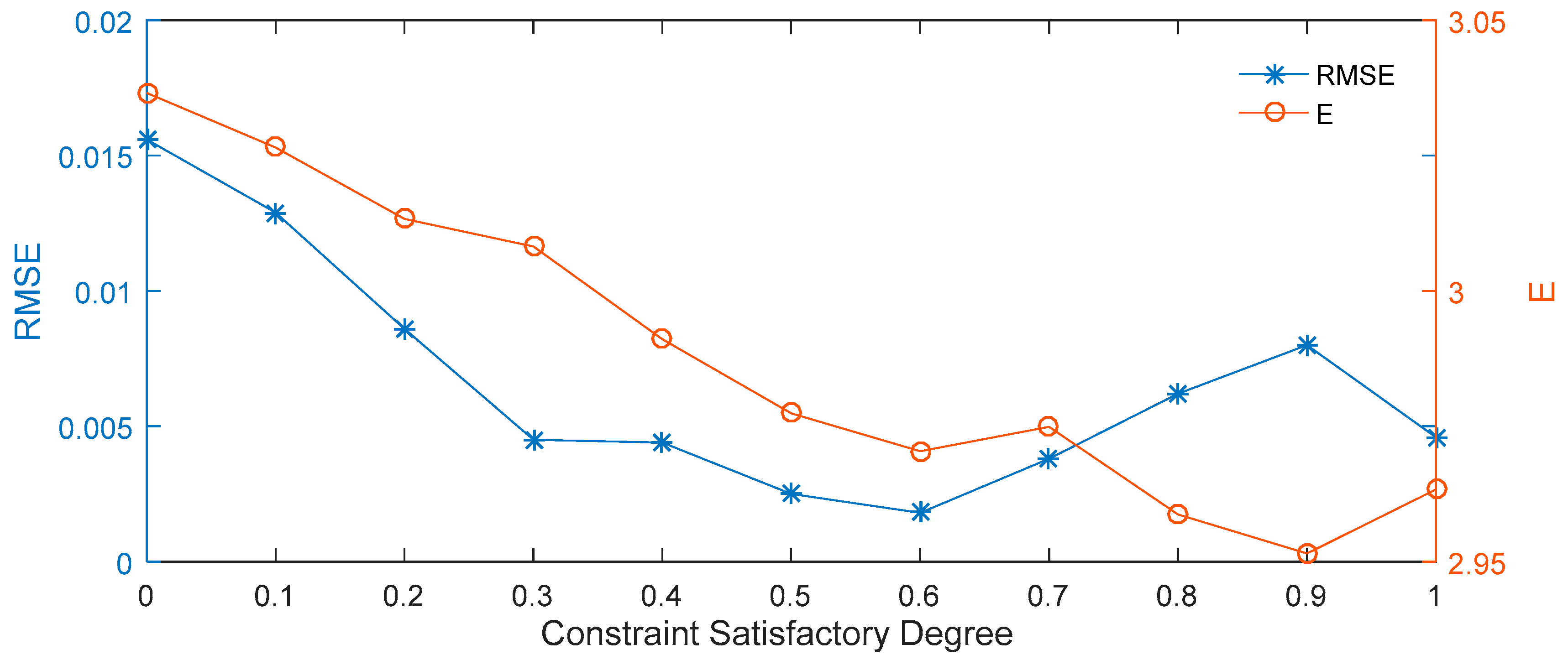
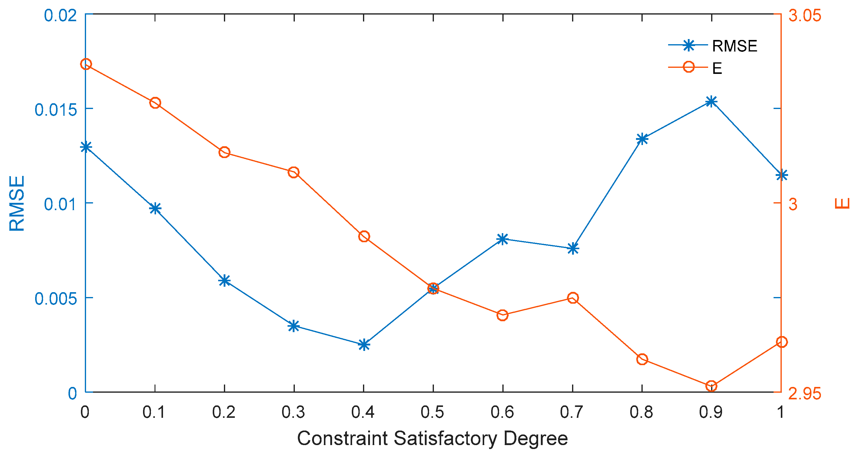
3.2. β Belonging to [0, 1]
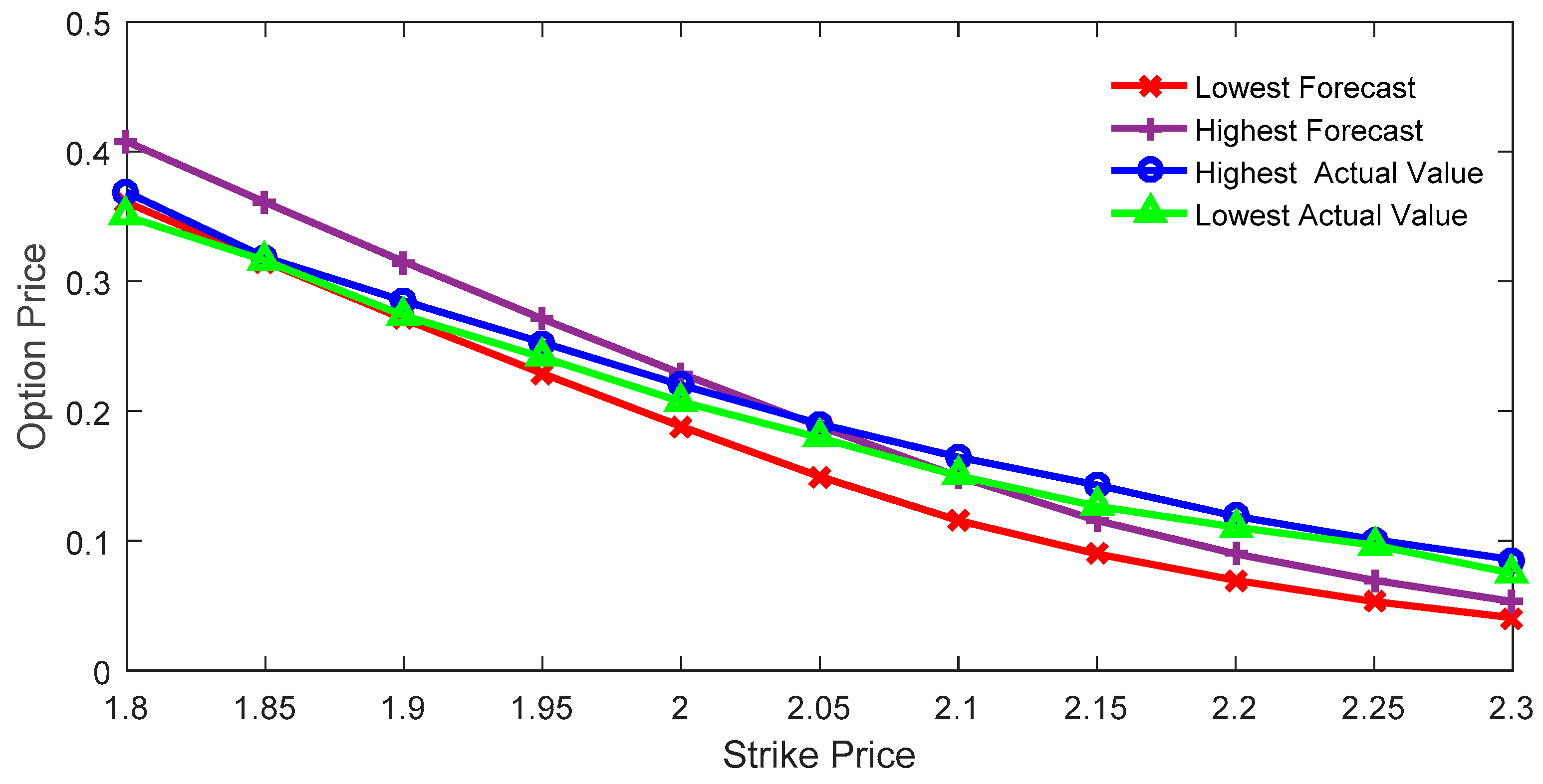
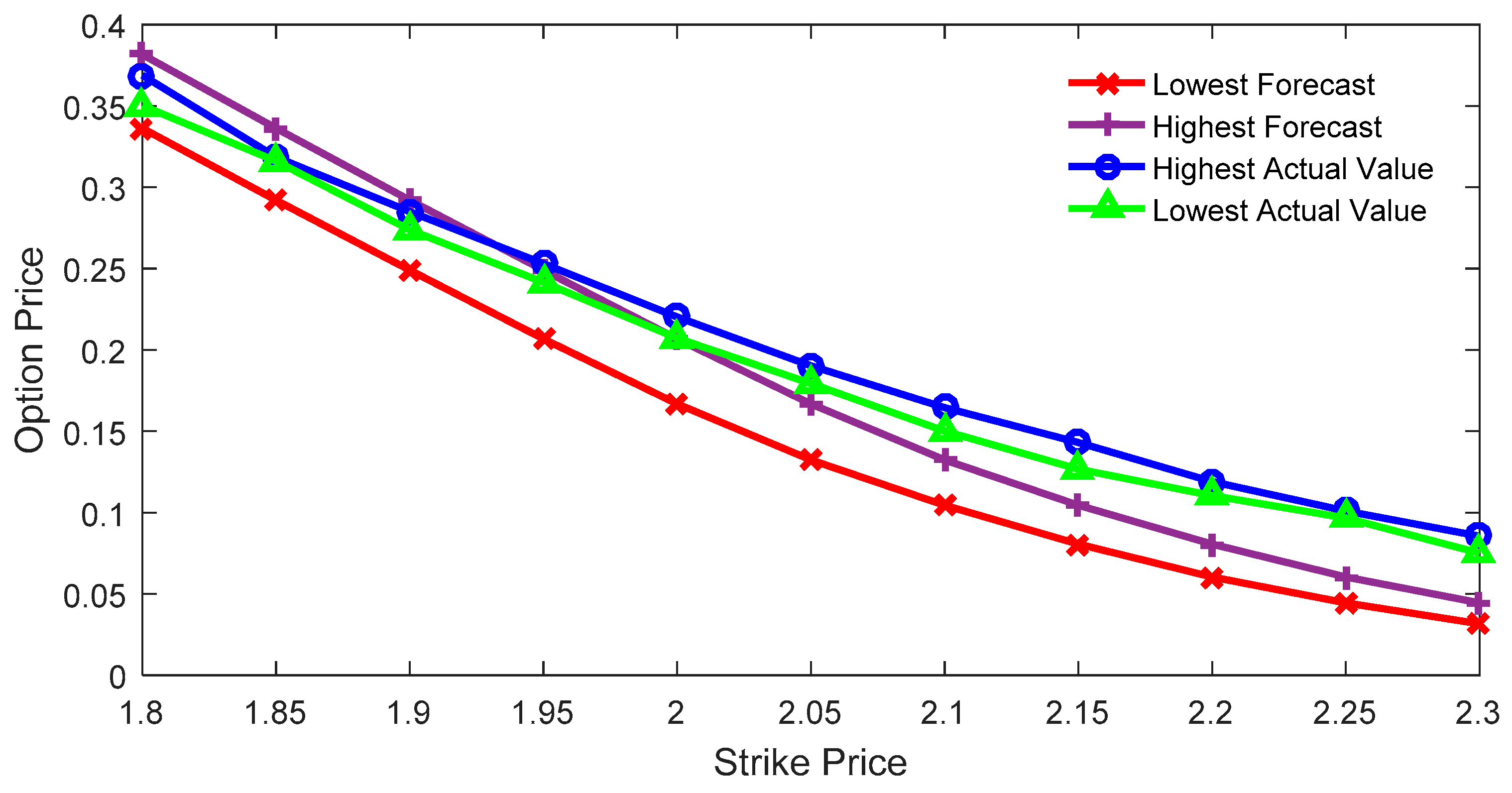
3.2.1. China SSE 50 ETF Option Pricing
3.2.2. US Boeing Stock Option Pricing
4. Conclusions
Author Contributions
Funding
Conflicts of Interest
References
- Fang, S.C.; Rajasekera, J.R.; Tsao, H.S.J. Entropy Optimization and Mathematical Programming; Springer: New York, NY, USA, 1997. [Google Scholar]
- Zhou, R.X.; Cai, R.; Tong, G.Q. Applications of entropy in finance: A Review. Entropy 2013, 15, 4909–4931. [Google Scholar] [CrossRef]
- He, X.J.; Zhu, S.P. Pricing European options with stochastic volatility under the minimal entropy martingale measure. Eur. J. Appl. Math. 2015, 27, 233–247. [Google Scholar] [CrossRef] [Green Version]
- Brody, D.C.; Buckley, L.R.C.; Constantinou, I.C. Option price calibration from Rényi entropy. Phys. Lett. A 2007, 366, 298–307. [Google Scholar] [CrossRef]
- Yu, X.S.; Xie, X.K. Pricing American options: RNMs-constrained entropic least-squares approach. N. Am. J. Econ. Financ. 2015, 31, 155–173. [Google Scholar] [CrossRef]
- Feunou, B.; Okou, C. Good volatility, bad volatility and option pricing. J. Financial Quant. Anal. 2019, 54, 695–727. [Google Scholar] [CrossRef]
- Zhang, M.; Wang, J.P.; Zhou, R.J. Entropy value-based pursuit projection cluster for the teaching quality evaluation with interval number. Entropy 2019, 21, 203. [Google Scholar] [CrossRef]
- Hernando, A.; Plastino, A.; Plastino, A.R. MaxEnt and dynamical information. Eur. Phys. J. B 2012, 85, 147. [Google Scholar] [CrossRef]
- Elith, J.; Phillips, S.J.; Hastie, T.; Dudík, M.; Chee, Y.E.; Yates, C.J. A statistical explanation of MaxEnt for ecologists. Divers. Distrib. 2011, 17, 43–57. [Google Scholar] [CrossRef]
- Zambrano, E.; Hernando, A.; Fernández Bariviera, A.; Hernando, R.; Plastino, A. Thermodynamics of firms’ growth. J. Royal Soc. Interface 2015, 12, 20150789. [Google Scholar] [CrossRef]
- Hu, Z.J.; Guo, K.; Jin, S.L.; Pan, H.H. The influence of climatic changes on distribution pattern of six typical Kobresia, species in Tibetan Plateau based on MaxEnt model and geographic information system. Theor. Appl. Climatol. 2018, 135, 375–390. [Google Scholar] [CrossRef]
- Raney, P.A.; Leopold, D.J. Fantastic Wetlands and Where to Find Them: Modeling Rich Fen Distribution in New York State with Maxent. Wetlands 2017, 38, 81–93. [Google Scholar] [CrossRef]
- Cozzolino, J.M.; Zahner, M.J. The maximum entropy distribution of the future market price of a stock. Oper. Res. 1973, 21, 1200–1211. [Google Scholar] [CrossRef]
- Bartiromo, R. Maximum entropy distribution of stock price fluctuations. Phys. A 2013, 392, 1638–1647. [Google Scholar] [CrossRef] [Green Version]
- Jackwerth, J.C.; Rubinstein, M. Recovering probability distributions from option prices. J. Financ. 1996, 51, 1611–1631. [Google Scholar] [CrossRef]
- Buchen, P.W.; Kelly, M. The maximum entropy distribution of an asset inferred from option prices. J. Financ. Quant. Anal. 1996, 31, 143–159. [Google Scholar] [CrossRef]
- Borwein, J.; Choksi, R.; MarEchal, P. Probability distributions of assets inferred from option prices via the principle of maximum entropy. SIAM J. Optim. 2003, 14, 464–478. [Google Scholar] [CrossRef]
- Rompolis, L.S. Retrieving risk neutral densities from European option prices based on the principle of maximum entropy. J. Empir. Financ. 2010, 17, 918–937. [Google Scholar] [CrossRef]
- Neri, C.; Schneider, L. Maximum entropy distributions inferred from option portfolios on an asset. Financ. Stoch. 2012, 16, 293–318. [Google Scholar] [CrossRef]
- Neri, C.; Schneider, L. A family of maximum entropy densities matching call option prices. Appl. Math. Financ. 2013, 20, 548–577. [Google Scholar] [CrossRef]
- Gulko, L. The entropic market hypothesis. Int. J. Theor. Appl. Financ. 1999, 2, 293–329. [Google Scholar] [CrossRef]
- Gulko, L. The entropy theory of stock option pricing. Int. J. Theor. Appl. Financ. 1999, 2, 331–355. [Google Scholar] [CrossRef]
- Tapiero, O.J. A maximum (non-extensive) entropy approach to equity options bid-ask spread. Phys. A 2013, 392, 3051–3060. [Google Scholar] [CrossRef]
- Liu, X.W.; Da, Q.L. A satisfactory solution for interval number linear programming. J. Syst. Eng. 1999, 2, 21–26. [Google Scholar]
- Zhou, R.X.; Liu, X.; Yu, M.; Li, J. Pricing option of Shanghai 50ETF based on the methods of maximum entropy and minimum cross-entropy. Math. Pract. Theory 2018, 48, 10–19. [Google Scholar]
- Kennedy, J.; Eberhart, R. Particle swarm optimization. In Proceedings of the IEEE International Conference on Neural Networks, Perth, Australia, 27 November–1 December 1995; pp. 1942–1948. [Google Scholar]
- Zhang, H.M.; Watada, J. An analysis of the arbitrage efficiency of the Chinese SSE 50ETF options market. Int. Rev. Econ. Financ. 2019, 59, 474–489. [Google Scholar] [CrossRef]
- Wang, J.Z.; Chen, S.J.; Tao, Q.Z.; Zhang, T. Modelling the implied volatility surface based on Shanghai 50ETF options. Econ. Model 2017, 64, 295–301. [Google Scholar] [CrossRef]


| 50ETF June Call Option | 50ETF September Call Option | |||||||
|---|---|---|---|---|---|---|---|---|
| Strike Price | Highest | Lowest | Strike Price | Highest | Lowest | Strike Price | Highest | Lowest |
| 1.80 | 0.3627 | 0.3400 | 2.25 | 0.0530 | 0.0436 | 1.80 | 0.3688 | 0.3502 |
| 1.85 | 0.3150 | 0.2928 | 2.30 | 0.0390 | 0.0321 | 1.85 | 0.3184 | 0.3160 |
| 1.90 | 0.2683 | 0.2492 | 2.35 | 0.0291 | 0.0241 | 1.90 | 0.2850 | 0.2737 |
| 1.95 | 0.2271 | 0.2066 | 2.40 | 0.0207 | 0.0162 | 1.95 | 0.2529 | 0.2415 |
| 2.00 | 0.1886 | 0.1684 | 2.45 | 0.0146 | 0.0115 | 2.00 | 0.2202 | 0.2072 |
| 2.05 | 0.1525 | 0.1329 | 2.50 | 0.0108 | 0.0085 | 2.05 | 0.1902 | 0.1793 |
| 2.10 | 0.1193 | 0.1061 | 2.55 | 0.0076 | 0.0061 | 2.10 | 0.1645 | 0.1501 |
| 2.15 | 0.0936 | 0.0801 | 2.60 | 0.0054 | 0.0045 | 2.15 | 0.1430 | 0.1266 |
| 2.20 | 0.0708 | 0.0605 | 2.65 | 0.0045 | 0.0036 | 2.20 | 0.1190 | 0.1105 |
| 2.25 | 0.1010 | 0.0966 | ||||||
| 2.30 | 0.0855 | 0.0750 | ||||||
| Strike Price | 2.50 | 2.55 | 2.60 | 2.65 | 2.70 | 2.75 | 2.80 | 2.85 | 2.90 | 2.95 | 3.00 | 3.10 | 3.20 | |
|---|---|---|---|---|---|---|---|---|---|---|---|---|---|---|
| Call option | Highest | 0.5309 | 0.4822 | 0.4350 | 0.3870 | 0.3425 | 0.2962 | 0.2520 | 0.2107 | 0.1740 | 0.1410 | 0.1122 | 0.0685 | 0.0400 |
| Lowest | 0.4927 | 0.4455 | 0.3988 | 0.3502 | 0.3067 | 0.2624 | 0.1900 | 0.1765 | 0.1405 | 0.1100 | 0.0842 | 0.0471 | 0.0262 | |
| Put option | Highest | 0.0062 | 0.0070 | 0.0088 | 0.0112 | 0.0143 | 0.0189 | 0.0254 | 0.0349 | 0.0481 | 0.0669 | 0.0901 | 0.1522 | 0.2287 |
| Lowest | 0.0047 | 0.0051 | 0.0068 | 0.0086 | 0.0104 | 0.0144 | 0.0200 | 0.0279 | 0.0401 | 0.0550 | 0.0750 | 0.1308 | 0.2031 | |
| β | 0.0 | 0.1 | 0.2 | 0.3 | 0.4 | 0.5 | 0.6 | 0.7 | 0.8 | 0.9 | 1.0 | |
|---|---|---|---|---|---|---|---|---|---|---|---|---|
| K | ||||||||||||
| 2.50 | 0.0032 | 0.0034 | 0.0060 | 0.0038 | 0.0042 | 0.0058 | 0.0042 | 0.0071 | 0.0052 | 0.0061 | 0.0054 | |
| 2.55 | 0.0042 | 0.0044 | 0.0079 | 0.0050 | 0.0055 | 0.0075 | 0.0055 | 0.0093 | 0.0068 | 0.0080 | 0.0070 | |
| 2.60 | 0.0053 | 0.0057 | 0.0099 | 0.0064 | 0.0070 | 0.0095 | 0.0070 | 0.0116 | 0.0087 | 0.0102 | 0.0088 | |
| 2.65 | 0.0069 | 0.0074 | 0.0122 | 0.0083 | 0.0090 | 0.0117 | 0.0092 | 0.0141 | 0.0111 | 0.0131 | 0.0108 | |
| 2.70 | 0.0090 | 0.0099 | 0.0148 | 0.0111 | 0.0117 | 0.0143 | 0.0121 | 0.0170 | 0.0145 | 0.0167 | 0.0134 | |
| 2.75 | 0.0121 | 0.0131 | 0.0180 | 0.0151 | 0.0152 | 0.0175 | 0.0155 | 0.0202 | 0.0189 | 0.0209 | 0.0165 | |
| 2.80 | 0.0159 | 0.0169 | 0.0219 | 0.0202 | 0.0195 | 0.0213 | 0.0198 | 0.0241 | 0.0247 | 0.0258 | 0.0207 | |
| 2.85 | 0.0211 | 0.0221 | 0.0275 | 0.0269 | 0.0258 | 0.0270 | 0.0268 | 0.0304 | 0.0326 | 0.0334 | 0.0284 | |
| 2.90 | 0.0295 | 0.0308 | 0.0367 | 0.0370 | 0.0364 | 0.0372 | 0.0385 | 0.0411 | 0.0434 | 0.0455 | 0.0405 | |
| 2.95 | 0.0412 | 0.0432 | 0.0497 | 0.0518 | 0.0515 | 0.0530 | 0.0550 | 0.0560 | 0.0599 | 0.0627 | 0.0585 | |
| 3.00 | 0.0566 | 0.0596 | 0.0673 | 0.0723 | 0.0706 | 0.0736 | 0.0769 | 0.0754 | 0.0840 | 0.0849 | 0.0813 | |
| 3.10 | 0.1044 | 0.1094 | 0.1176 | 0.1256 | 0.1244 | 0.1301 | 0.1356 | 0.1321 | 0.1436 | 0.1453 | 0.1414 | |
| 3.20 | 0.1612 | 0.1686 | 0.1782 | 0.1889 | 0.1905 | 0.1993 | 0.2054 | 0.2015 | 0.2145 | 0.2189 | 0.2120 | |
| RMSE | 0.0156 | 0.0129 | 0.0086 | 0.0045 | 0.0044 | 0.0025 | 0.0018 | 0.0038 | 0.0062 | 0.0080 | 0.0046 | |
| E | 3.0366 | 3.0265 | 3.0133 | 3.0082 | 2.9911 | 2.9774 | 2.9704 | 2.9749 | 2.9587 | 2.9515 | 2.9633 | |
| β | 0.0 | 0.1 | 0.2 | 0.3 | 0.4 | 0.5 | 0.6 | 0.7 | 0.8 | 0.9 | 1.0 | |
|---|---|---|---|---|---|---|---|---|---|---|---|---|
| K | ||||||||||||
| 2.50 | 0.0042 | 0.0044 | 0.0079 | 0.0050 | 0.0055 | 0.0075 | 0.0055 | 0.0093 | 0.0068 | 0.0080 | 0.0070 | |
| 2.55 | 0.0053 | 0.0057 | 0.0099 | 0.0064 | 0.0070 | 0.0095 | 0.0070 | 0.0116 | 0.0087 | 0.0102 | 0.0088 | |
| 2.60 | 0.0069 | 0.0074 | 0.0122 | 0.0083 | 0.0090 | 0.0117 | 0.0092 | 0.0141 | 0.0111 | 0.0131 | 0.0108 | |
| 2.65 | 0.0090 | 0.0099 | 0.0148 | 0.0111 | 0.0117 | 0.0143 | 0.0121 | 0.0170 | 0.0145 | 0.0167 | 0.0134 | |
| 2.70 | 0.0121 | 0.0131 | 0.0180 | 0.0151 | 0.0152 | 0.0175 | 0.0155 | 0.0202 | 0.0189 | 0.0209 | 0.0165 | |
| 2.75 | 0.0159 | 0.0169 | 0.0219 | 0.0202 | 0.0195 | 0.0213 | 0.0198 | 0.0241 | 0.0247 | 0.0258 | 0.0207 | |
| 2.80 | 0.0211 | 0.0221 | 0.0275 | 0.0269 | 0.0258 | 0.0270 | 0.0268 | 0.0304 | 0.0326 | 0.0334 | 0.0284 | |
| 2.85 | 0.0295 | 0.0308 | 0.0367 | 0.0370 | 0.0364 | 0.0372 | 0.0385 | 0.0411 | 0.0434 | 0.0455 | 0.0405 | |
| 2.90 | 0.0412 | 0.0432 | 0.0497 | 0.0518 | 0.0515 | 0.0530 | 0.0550 | 0.0560 | 0.0599 | 0.0627 | 0.0585 | |
| 2.95 | 0.0566 | 0.0596 | 0.0673 | 0.0723 | 0.0706 | 0.0736 | 0.0769 | 0.0754 | 0.0840 | 0.0849 | 0.0813 | |
| 3.00 | 0.0783 | 0.0821 | 0.0901 | 0.0972 | 0.0950 | 0.0994 | 0.1042 | 0.1012 | 0.1122 | 0.1127 | 0.1094 | |
| 3.10 | 0.1324 | 0.1386 | 0.1474 | 0.1564 | 0.1566 | 0.1638 | 0.1697 | 0.1659 | 0.1780 | 0.1812 | 0.1760 | |
| 3.20 | 0.1909 | 0.1993 | 0.2099 | 0.2226 | 0.2255 | 0.2360 | 0.2424 | 0.2382 | 0.2522 | 0.2578 | 0.2490 | |
| RMSE | 0.0130 | 0.0097 | 0.0059 | 0.0035 | 0.0025 | 0.0055 | 0.0081 | 0.0076 | 0.0134 | 0.0154 | 0.0115 | |
| E | 3.0366 | 3.0265 | 3.0133 | 3.0082 | 2.9911 | 2.9774 | 2.9704 | 2.9749 | 2.9587 | 2.9515 | 2.9633 | |
| Strike Price | 3.425 | 3.450 | 3.500 | 3.550 | 3.575 | 3.600 | 3.625 | 3.650 | 3.675 | 3.700 | |
|---|---|---|---|---|---|---|---|---|---|---|---|
| Call option | Highest | 0.1720 | 0.1615 | 0.1241 | 0.0900 | 0.0720 | 0.0610 | 0.0490 | 0.0395 | 0.0305 | 0.0231 |
| Lowest | 0.1615 | 0.1351 | 0.0991 | 0.0697 | 0.0575 | 0.0470 | 0.0385 | 0.0296 | 0.0225 | 0.0165 | |
| Put option | Highest | 0.0261 | 0.0316 | 0.0463 | 0.0700 | 0.0780 | 0.0925 | 0.1075 | 0.1195 | 0.1335 | 0.1606 |
| Lowest | 0.0170 | 0.0205 | 0.0315 | 0.0479 | 0.0585 | 0.0690 | 0.0855 | 0.0985 | 0.1203 | 0.1323 | |
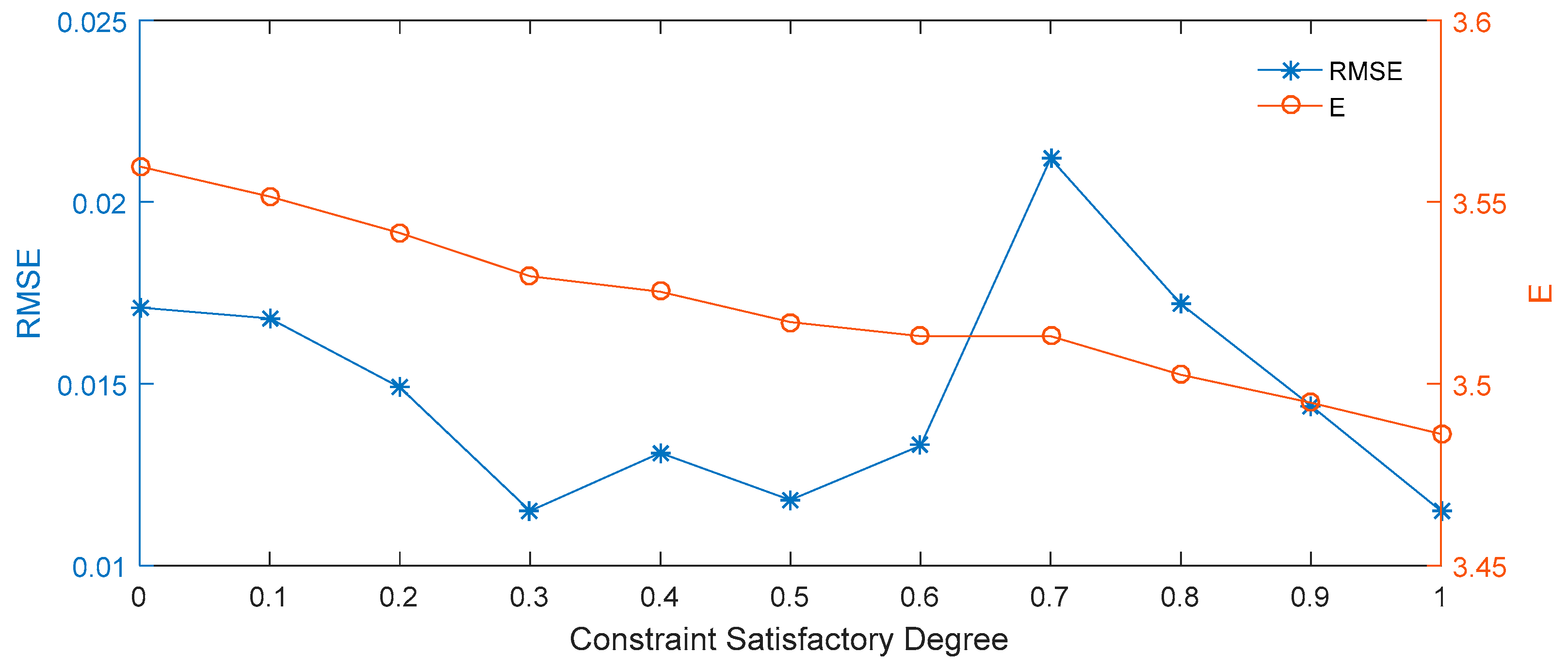
| β | 0.0 | 0.1 | 0.2 | 0.3 | 0.4 | 0.5 | 0.6 | 0.7 | 0.8 | 0.9 | 1.0 | |
|---|---|---|---|---|---|---|---|---|---|---|---|---|
| K | ||||||||||||
| 3.425 | 0.0152 | 0.0150 | 0.0157 | 0.0173 | 0.0157 | 0.0147 | 0.0117 | 0.0010 | 0.0010 | 0.0010 | 0.0011 | |
| 3.450 | 0.0197 | 0.0194 | 0.0203 | 0.0224 | 0.0204 | 0.0191 | 0.0152 | 0.0033 | 0.0033 | 0.0035 | 0.0038 | |
| 3.500 | 0.0305 | 0.0301 | 0.0313 | 0.0343 | 0.0311 | 0.0291 | 0.0241 | 0.0126 | 0.0130 | 0.0139 | 0.0153 | |
| 3.550 | 0.0436 | 0.0431 | 0.0448 | 0.0485 | 0.0442 | 0.0423 | 0.0372 | 0.0281 | 0.0294 | 0.0314 | 0.0345 | |
| 3.575 | 0.0510 | 0.0505 | 0.0525 | 0.0565 | 0.0520 | 0.0506 | 0.0462 | 0.0386 | 0.0404 | 0.0432 | 0.0472 | |
| 3.600 | 0.0591 | 0.0587 | 0.0608 | 0.0651 | 0.0607 | 0.0601 | 0.0569 | 0.0507 | 0.0534 | 0.0570 | 0.0616 | |
| 3.625 | 0.0679 | 0.0678 | 0.0700 | 0.0746 | 0.0706 | 0.0713 | 0.0695 | 0.0642 | 0.0679 | 0.0722 | 0.0775 | |
| 3.650 | 0.0777 | 0.0779 | 0.0804 | 0.0851 | 0.0820 | 0.0840 | 0.0834 | 0.0787 | 0.0834 | 0.0882 | 0.0942 | |
| 3.675 | 0.0885 | 0.0893 | 0.0921 | 0.0971 | 0.0953 | 0.0983 | 0.0986 | 0.0944 | 0.1001 | 0.1054 | 0.1118 | |
| 3.700 | 0.1006 | 0.1021 | 0.1054 | 0.1108 | 0.1106 | 0.1144 | 0.1151 | 0.1114 | 0.1182 | 0.1236 | 0.1307 | |
| RMSE | 0.0171 | 0.0168 | 0.0149 | 0.0115 | 0.0131 | 0.0118 | 0.0133 | 0.0212 | 0.0172 | 0.0144 | 0.0116 | |
| E | 3.5598 | 3.5515 | 3.5415 | 3.5296 | 3.5253 | 3.5170 | 3.5131 | 3.5131 | 3.5025 | 3.4948 | 3.4862 | |
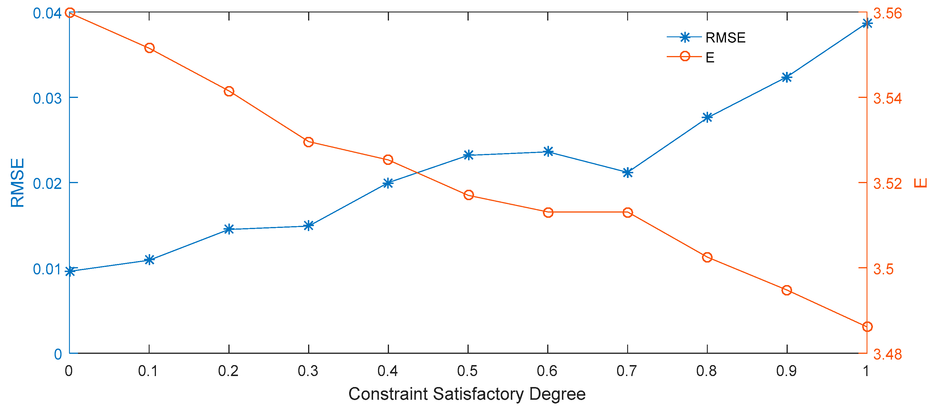
| β | 0.0 | 0.1 | 0.2 | 0.3 | 0.4 | 0.5 | 0.6 | 0.7 | 0.8 | 0.9 | 1.0 | |
|---|---|---|---|---|---|---|---|---|---|---|---|---|
| K | ||||||||||||
| 3.425 | 0.0368 | 0.0363 | 0.0378 | 0.038 | 0.0372 | 0.0352 | 0.0300 | 0.0196 | 0.0204 | 0.0218 | 0.0240 | |
| 3.450 | 0.0436 | 0.0431 | 0.0448 | 0.0485 | 0.0442 | 0.0423 | 0.0372 | 0.0281 | 0.0294 | 0.0314 | 0.0345 | |
| 3.500 | 0.0591 | 0.0587 | 0.0608 | 0.0601 | 0.0607 | 0.0601 | 0.0569 | 0.0507 | 0.0534 | 0.0570 | 0.0616 | |
| 3.550 | 0.0777 | 0.0779 | 0.0804 | 0.0801 | 0.0820 | 0.0840 | 0.0834 | 0.0787 | 0.0834 | 0.0882 | 0.0942 | |
| 3.575 | 0.0885 | 0.0893 | 0.0921 | 0.0914 | 0.0953 | 0.0983 | 0.0986 | 0.0944 | 0.1001 | 0.1054 | 0.1118 | |
| 3.600 | 0.1006 | 0.1021 | 0.1054 | 0.1058 | 0.1106 | 0.1144 | 0.1151 | 0.1114 | 0.1182 | 0.1236 | 0.1307 | |
| 3.625 | 0.1141 | 0.1164 | 0.1205 | 0.1127 | 0.1278 | 0.1322 | 0.1331 | 0.1299 | 0.1376 | 0.1433 | 0.1509 | |
| 3.650 | 0.1290 | 0.1321 | 0.1371 | 0.1411 | 0.1462 | 0.1510 | 0.1523 | 0.1495 | 0.1580 | 0.1641 | 0.1721 | |
| 3.675 | 0.1451 | 0.1488 | 0.1550 | 0.1552 | 0.1654 | 0.1706 | 0.1724 | 0.1702 | 0.1794 | 0.1859 | 0.1942 | |
| 3.700 | 0.1619 | 0.1664 | 0.1737 | 0.1744 | 0.1853 | 0.1911 | 0.1933 | 0.1918 | 0.2017 | 0.2085 | 0.2170 | |
| RMSE | 0.0096 | 0.0109 | 0.0145 | 0.0149 | 0.0200 | 0.0232 | 0.0236 | 0.0212 | 0.0276 | 0.0324 | 0.0387 | |
| E | 3.5598 | 3.5515 | 3.5415 | 3.5296 | 3.5253 | 3.5170 | 3.5131 | 3.5131 | 3.5025 | 3.4948 | 3.4862 | |
© 2019 by the authors. Licensee MDPI, Basel, Switzerland. This article is an open access article distributed under the terms and conditions of the Creative Commons Attribution (CC BY) license (http://creativecommons.org/licenses/by/4.0/).
Share and Cite
Liu, X.; Zhou, R.; Xiong, Y.; Yang, Y. Pricing Interval European Option with the Principle of Maximum Entropy. Entropy 2019, 21, 788. https://doi.org/10.3390/e21080788
Liu X, Zhou R, Xiong Y, Yang Y. Pricing Interval European Option with the Principle of Maximum Entropy. Entropy. 2019; 21(8):788. https://doi.org/10.3390/e21080788
Chicago/Turabian StyleLiu, Xiao, Rongxi Zhou, Yahui Xiong, and Yuexiang Yang. 2019. "Pricing Interval European Option with the Principle of Maximum Entropy" Entropy 21, no. 8: 788. https://doi.org/10.3390/e21080788