Geometric Estimation of Multivariate Dependency

Abstract

This paper proposes a geometric estimator of dependency between a pair of multivariate random variables. The proposed estimator of dependency is based on a randomly permuted geometric graph (the minimal spanning tree) over the two multivariate samples. This estimator converges to a quantity that we call the geometric mutual information (GMI), which is equivalent to the Henze–Penrose divergence. between the joint distribution of the multivariate samples and the product of the marginals. The GMI has many of the same properties as standard MI but can be estimated from empirical data without density estimation; making it scalable to large datasets. The proposed empirical estimator of GMI is simple to implement, involving the construction of an minimal spanning tree (MST) spanning over both the original data and a randomly permuted version of this data. We establish asymptotic convergence of the estimator and convergence rates of the bias and variance for smooth multivariate density functions belonging to a Hölder class. We demonstrate the advantages of our proposed geometric dependency estimator in a series of experiments.

1. Introduction

Estimation of multivariate dependency has many applications in fields such as information theory, clustering, structure learning, data processing, feature selection, time series prediction, and reinforcement learning, see [1,2,3,4,5,6,7,8,9,10], respectively. It is difficult to accurately estimate the mutual information in high-dimensional settings, specially where the data is multivariate with an absolutely continuous density with respect to Lebesgue measure—the setting considered in this paper. An important and regular measure of dependency is the Shannon mutual information (MI), which has seen extensive use across many application domains. However, the estimation of mutual information can often be challenging. In this paper, we focus on a measure of MI that we call the Geometric MI (GMI). This MI measure is defined as the asymptotic large sample limit of a randomized minimal spanning tree (MST) statistic spanning the multivariate sample realizations. The GMI is related to a divergence measure called the Henze–Penrose divergence [11,12], and related to the multivariate runs test [13]. In [14,15], it was shown that this divergence measure can be used to specify a tighter bound for the Bayes error rate for testing if a random sample comes from one of two distributions the bound in [14,15] is tighter than previous divergence-type bounds such as the Bhattacharrya bound [16]. Furthermore, the authors of [17] proposed a non-parametric bound on multi-class classification Bayes error rate using a global MST graph.

Let $\mathbf{X}$ and $\mathbf{Y}$ be random variables with unknown joint density $f_{XY}$ and marginal densities $f_X$ and $f_Y$, respectively, and consider two hypotheses: $H_0$, $\mathbf{X}$ and $\mathbf{Y}$ are independent and $H_1$, $\mathbf{X}$ and $\mathbf{Y}$ are dependent,

$$H_0:f_{XY}=f_X{f}_Y,\mathrm{versus}{H}_1:f_{XY}\ne f_X{f}_Y.$$

The GMI is defined as the Henze–Penrose divergence between $f_{XY}$ and $f_X{f}_Y$ which can be used as a dependency measure. In this paper, we prove that for large sample size n the randomized MST statistic spanning the original multivariate sample realizations and a randomly shuffled data set converges almost surely to the GMI measure. A direct implication of [14,15] is that the GMI provides a tighter bound on the Bayes misclassification rate for the optimal test of independence. In this paper, we propose an estimator based on a random permutation modification of the Friedman–Rafsky multivariate test statistic and show that under certain conditions the GMI estimator achieves the parametric mean square error (MSE) rate when the joint density is bounded and smooth. Importantly unlike other measures of MI, our proposed GMI estimator does not require explicit estimation of the joint and marginal densities.

Computational complexity is an important challenge in machine learning and data science. Most plug-in-based estimators, such as the kernel density estimator (KDE) or the K-nearest-neighbor (KNN) estimator with known convergence rate, require runtime complexity of $O(n^2)$, which is not suitable for large scale applications. Noshad et al. proposed a graph theoretic direct estimation method based on nearest-neighbor ratios (NNR) [18]. The NNR estimator is based on k-NN graph and computationally more tractable than other competing estimators with complexity $O(knlogn)$. The construction of the minimal spanning tree lies at the heart of the GMI estimator proposed in this paper. Since the GMI estimator is based on the Euclidean MST the dual-tree algorithm by March et al. [19] can be applied. This algorithm is based on the construction of Borůvka [20] and implements the Euclidean MST in approximately $O(nlogn)$ time. In this paper, we experimentally show that for large sample size the proposed GMI estimator has faster runtime than the KDE plug-in method.

1.1. Related Work

Estimation of mutual information has a rich history. The most common estimators of MI are based on plug-in density estimation, e.g., using the histogram, kernel density or kNN density estimators [21,22]. Motivated by ensemble methods applied to divergence estimation [23,24], in [22] an ensemble method for combining multiple KDE bandwidths was proposed for estimating MI. Under certain smoothness conditions this ensemble MI estimator was shown to achieve parametric convergence rates.

Another class of estimators of multivariate dependency bypasses the difficult density estimation task. This class includes the statistically consistent estimators of Rényi-$\alpha$ and KL mutual information which are motivated by the asymptotic limit of the length of the KNN graph, [25,26] when joint density is smooth. The estimator of [27] builds on KNN methods for Rényi entropy estimation. The authors of [26], showed that when MI is large the KNN and KDE approaches are ill-suited for estimating MI since the joint density may be insufficiently smooth when there are strong dependencies. To overcome this issue an assumption on the smoothness of the density is required, see [28,29], and [23,24]. For all these methods, the optimal parametric rate of MSE convergence is achieved when the densities are either d, $(d+1)/2$ or $d/2$ times differentiable [30]. In this paper, we assume that joint and marginal densities are smooth in the sense that they belong to Hölder continuous classes of densities ${\mathsf{\Sigma }}_d(\eta ,K)$, where the smoothness parameter $\eta \in (0,1]$ and the Lipschitz constant $K>0$.

A MI measure based on the Pearson chi-square divergence was considered in [31] that is computational efficient and numerically stable. The authors of [27,32] used nearest-neighbor graph and minimal spanning tree approaches, respectively, to estimate Rényi mutual information. In [22], a non-parametric mutual information estimator was proposed using a weighted ensemble method with $O(1/n)$ parametric convergence rate. This estimator was based on plug-in density estimation, which is challenging in high dimension.

Our proposed dependency estimator differs from previous methods in the following ways. First, it estimates a different measure of mutual information, the GMI. Second, instead of using the KNN graph the estimator of GMI uses a randomized minimal spanning tree that spans the multivariate realizations. The proposed GMI estimator is motivated by the multivariate runs test of Friedman and Rafsky (FR) [33] which is a multivariate generalization of the univariate Smirnov maximum deviation test [34] and the Wald-Wolfowitz [35] runs test in one dimension. We also emphasize that the proposed GMI estimator does not require boundary correction, in contrast to other graph-based estimators, such as, the NNR estimator [18], scalable MI estimator [36], or cross match statistic [37].

1.2. Contribution

The contribution of this paper has three components

(1)

We propose a novel non-parametric multivariate dependency measure, referred to as geometric mutual information (GMI), which is based on graph-based divergence estimation. The geometric mutual information is constructed using a minimal spanning tree and is a function of the Friedman–Rafsky multivariate test statistic.

(2)

We establish properties of the proposed dependency measure analogous to those of Shannon mutual information, such as, convexity, concavity, chain rule, and a type of data-processing inequality.

(3)

We derive a bound on the MSE rate for the proposed geometric estimator. An advantage of the estimator is that it achieves the optimal MSE rate without the need for boundary correction, which is required for most plug-in estimators.

1.3. Organization

The rest of the paper is organized as follows. In Section 2, we define the geometric mutual information and establish some of its mathematical properties. In Section 2.2 and Section 2.3, we introduce a statistically consistent GMI estimator and derive a bound on its mean square error convergence rate. In Section 3 we verify the theory through experiments.

Throughout the paper, we denote statistical expectation by $\mathbb{E}$ and the variance by abbreviation $\mathrm{Var}$. Bold face type indicates random vectors. All densities are assumed to be absolutely continuous with respect to non-atomic Lebesgue measure.

2. The Geometric Mutual Information (GMI)

In this section, we first review the definition of the Henze–Penrose (HP) divergence measure defined by Berisha and Hero in [13,14]. The Henze–Penrose divergence between densities f and g with domain ${\mathbb{R}}^d$ for parameter $p\in (0,1)$ is defined as follows (see [13,14,15]):

$${\displaystyle D_p(f,g)=\frac{1}{4pq}\left[\int \frac{{\left(pf(\mathbf{x})-qg(\mathbf{x})\right)}^2}{pf(\mathbf{x})+qg(\mathbf{x})}\mathrm{d}\mathbf{x}-{(p-q)}^2\right],}$$

(1)

where $q=1-p$. This functional is an f-divergence [38], equivalently, as an Ali-Silvey distance [39], i.e., it satisfies the properties of non-negativity, monotonicity, and joint convexity [15]. The measure (1) takes values in $[0,1]$ and $D_p(f,g)=0$ if and only if $f=g$ almost surely.

The mutual information measure is defined as follows. Let $f_X$, $f_Y$, and $f_{XY}$ be the marginal and joint distributions, respectively, of random vectors $\mathbf{X}\in {\mathbb{R}}^{d_x}$, $\mathbf{Y}\in {\mathbb{R}}^{d_y}$ where $d_x$ and $d_y$ are positive integers. Then by using (1), a Henze–Penrose generalization of the mutual information between $\mathbf{X}$ and $\mathbf{Y}$, is defined by

$$\begin{array}{cc}\hfill I_p(\mathbf{X};\mathbf{Y})& =D_p(f_{XY},f_X{f}_Y)\hfill \\ & {\displaystyle =\frac{1}{4pq}\left[\int \int \frac{{\left(p{f}_{XY}(\mathbf{x},\mathbf{y})-q{f}_X(\mathbf{y})f_Y(\mathbf{y})\right)}^2}{p{f}_{XY}(\mathbf{x},\mathbf{y})+q{f}_X(\mathbf{x})f_Y(\mathbf{y})}\mathrm{d}\mathbf{x}\mathrm{d}\mathbf{y}-{(p-q)}^2\right].}\hfill \end{array}$$

(2)

We will show below that $I_p(\mathbf{X};\mathbf{Y})$ has a geometric interpretation in terms of the large sample limit of a minimal spanning tree spanning n sample realizations of the merged labeled samples $\mathbf{X}\cup \mathbf{Y}$. Thus, we call $I_p(\mathbf{X};\mathbf{Y})$ the GMI between $\mathbf{X}$ and $\mathbf{Y}$. The GMI satisfies similar properties to other definitions of mutual information, such as Shannon and Rényi mutual information. Recalling (3) in [14], an alternative form of $I_p$ is given by

$$\begin{array}{c}\hfill {\displaystyle I_p(\mathbf{X};\mathbf{Y})=1-A_p(\mathbf{X};\mathbf{Y})=\frac{u_p(\mathbf{X};\mathbf{Y})}{4pq}-\frac{{(p-q)}^2}{4pq},}\end{array}$$

(3)

where

$$\begin{array}{c}{\displaystyle A_p(\mathbf{X};\mathbf{Y})=\int \int \frac{f_{XY}(\mathbf{x},\mathbf{y})f_X(\mathbf{x})f_Y(\mathbf{y})}{p{f}_{XY}(\mathbf{x},\mathbf{y})+q{f}_X(\mathbf{x})f_Y(\mathbf{y})}\mathrm{d}\mathbf{x}\mathrm{d}\mathbf{y}={\mathbb{E}}_{XY}\left[{\left(p\frac{f_{XY}(\mathbf{X},\mathbf{Y})}{f_X(\mathbf{X})f_Y(\mathbf{Y})}+q\right)}^{-1}\right],\mathrm{and}}\\ {\displaystyle u_p(\mathbf{X};\mathbf{Y})={\displaystyle \int \int \frac{{\left(p{f}_{XY}(\mathbf{x},\mathbf{y})-q{f}_X(\mathbf{x})f_Y(\mathbf{y})\right)}^2}{p{f}_{XY}(\mathbf{x},\mathbf{y})+q{f}_X(\mathbf{x})f_Y(\mathbf{y})}\mathrm{d}\mathbf{x}\mathrm{d}\mathbf{y}}=1-4pq{A}_p(\mathbf{X};\mathbf{Y}).}\end{array}$$

(4)

The function $A_p(\mathbf{X};\mathbf{Y})$ was defined in [13] and is called the geometric affinity between $\mathbf{X}$ and $\mathbf{Y}$. The next subsection of the paper is dedicated to the basic inequalities and properties of the proposed GMI measure (2).

2.1. Properties of the Geometric Mutual Information

In this subsection we establish basic inequalities and properties of the GMI, $I_p$, given in (2). The following theorem shows that $I_p(\mathbf{X};\mathbf{Y})$ is a concave function in $f_X$ and a convex function in $f_{Y|X}$. The proof is given in Appendix A.1.

Theorem 1.

Denote by ${\tilde{I}}_p(f_{XY})$ the GMI $I_p(\mathbf{X};\mathbf{Y})$ when $\mathbf{X}\in {\mathbb{R}}^{d_x}$ and $\mathbf{Y}\in {\mathbb{R}}^{d_y}$ have joint density $f_{XY}$. Then the GMI satisfies

(i)

Concavity in $f_X$: Let $f_{Y|X}$ be conditional density of $\mathbf{Y}$ given $\mathbf{X}$ and let $g_X$ and $h_X$ be densities on ${\mathbb{R}}^{d_x}$. Then for ${\lambda }_1,{\lambda }_2\in [0,1]$, ${\lambda }_1+{\lambda }_2=1$

$${\tilde{I}}_p\left({\lambda }_1{f}_{Y|X}{g}_X+{\lambda }_2{f}_{Y|X}{h}_X\right)\ge {\lambda }_1{\tilde{I}}_p(f_{Y|X}{g}_X)+{\lambda }_2{\tilde{I}}_p(f_{Y|X}{h}_X).$$

(5)

The inequality is strict unless either ${\lambda }_1$ or ${\lambda }_2$ are zero or $h_X=g_X$.

(ii)

Convexity in $f_{Y|X}$: Let $g_{Y|X}$ and $h_{Y|X}$ be conditional densities of $\mathbf{Y}$ given $\mathbf{X}$ and let $f_X$ be marginal density. Then for ${\lambda }_1,{\lambda }_2\in [0,1]$, ${\lambda }_1+{\lambda }_2=1$

$${\tilde{I}}_p\left({\lambda }_1{g}_{Y|X}{f}_X+{\lambda }_2{h}_{Y|X}{f}_X\right)\le {\lambda }_1{\tilde{I}}_p(g_{Y|X}{f}_X)+{\lambda }_2{\tilde{I}}_p(h_{Y|X}{f}_X).$$

(6)

The inequality is strict unless either ${\lambda }_1$ or ${\lambda }_2$ are zero or $h_{Y|X}=g_{Y|X}$.

The GMI, $I_p(\mathbf{X};\mathbf{Y})$, satisfies properties analogous to the standard chain rule and the data-processing inequality [40]. For random variables $\mathbf{X}\in {\mathbb{R}}^{d_x},\mathbf{Y}\in {\mathbb{R}}^{d_y}$, and $\mathbf{Z}\in {\mathbb{R}}^{d_z}$ with conditional density $f_{XY|Z}$ we define the conditional GMI

$$\begin{array}{c}{\displaystyle I_p(\mathbf{X};\mathbf{Y}|\mathbf{Z})={\mathbb{E}}_{\mathbf{Z}}\left[{\tilde{I}}_p(f_{XY|Z})\right],\mathrm{where}}\hfill \\ {\displaystyle {\tilde{I}}_p(f_{XY|Z})=1-\int \int \frac{f_{XY|Z}(\mathbf{x},\mathbf{y}|\mathbf{z})f_{X|Z}(\mathbf{x}|\mathbf{z})f_{Y|Z}(\mathbf{y}|\mathbf{z})}{p{f}_{XY|Z}(\mathbf{x},\mathbf{y}|\mathbf{z})+q{f}_{X|Z}(\mathbf{x}|\mathbf{z})f_{Y|Z}(\mathbf{y}|\mathbf{z})}\mathrm{d}\mathbf{x}\mathrm{d}\mathbf{y}.}\hfill \end{array}$$

(7)

The next theorem establishes a relation between the joint and conditional GMI.

Theorem 2.

For given d-dimensional random vector $\mathbf{X}$ with components $X_1,X_2,\cdots ,X_d$ and random variable Y,

$$I_p(\mathbf{X};Y)\ge I_p(X_1;Y)-{\displaystyle \sum _{i=1}^{d-1}\left(1-I_p(X_i;Y|{\mathbf{X}}^{i-1})\right)},$$

(8)

where ${\mathbf{X}}^i:=X_1,X_2,\cdots ,X_i$ and the conditional GMI $I_p(X_i;Y|{\mathbf{X}}^{i-1})$ is defined in (7).

For $d=2$ Theorem 2 reduces to

$$I_p(X_1,X_2;Y)\ge I_p(X_1;Y)-\left(1-I_p(X_2;Y|X_1)\right),$$

(9)

Please note that when ${\displaystyle {\displaystyle \sum _{i=1}^{d-1}\left(1-I_p(X_i;Y|{\mathbf{X}}^{i-1})\right)}\ge 1}$, the inequality (8) is trivial since $0\le I_p(X_1;Y)\le 1$. The proof of Theorem 2 is given in Appendix A.2. Theorem 2 is next applied to the case where $\mathbf{X}$ and $\mathbf{Y}$ form a Markov chain. The proof of the following “leany” data-processing inequality (Proposition 1) is provided in Appendices section, Appendix A.3.

Proposition 1.

Suppose random vectors $\mathbf{X},\mathbf{Y},\mathbf{Z}$ form a Markov chain denoted, $\mathbf{X}\to \mathbf{Y}\to \mathbf{Z}$, in the sense that $f_{XYZ}=f_{X|Y}{f}_{Y|Z}{f}_Z$. Then for $p\in (0,1)$

$$I_p(\mathbf{Y};\mathbf{X})\ge I_p(\mathbf{Z};\mathbf{X})-{\left(p{\mathbb{E}}_{XY}\left[{\delta }_{X,Y}\right]+(1-p)\right)}^{-1},$$

(10)

where

$${\displaystyle {\delta }_{X,Y}=\int \frac{f_{X|Y}(\mathbf{X}|\mathbf{Y})f_{Z|Y}(\mathbf{z}|\mathbf{Y})}{f_{X|Z}(\mathbf{X}|\mathbf{z})}\mathrm{d}\mathbf{z}.}$$

Furthermore, if both $\mathbf{X}\to \mathbf{Y}\to \mathbf{Z}$ and $\mathbf{X}\to \mathbf{Z}\to \mathbf{Y}$ together hold true, we have $I_p(\mathbf{Y};\mathbf{X})=I_p(\mathbf{Z};\mathbf{X})$.

The inequality in (10) becomes interpretable as the standard data-processing inequality $I_p(\mathbf{Y};\mathbf{X})\ge I_p(\mathbf{Z};\mathbf{X})$, when

$${\mathbb{E}}_Z\left[\frac{f(\mathbf{Z}|\mathbf{Y})}{f(\mathbf{Z}|\mathbf{X})}\right]=\infty ,$$

since

$${\mathbb{E}}_{XY}\left[{\delta }_{X,Y}\right]={\mathbb{E}}_{XY}\left({\displaystyle \frac{f(\mathbf{X}|\mathbf{Y})}{f(\mathbf{X})}{\mathbb{E}}_Z\left[\frac{f(\mathbf{Z}|\mathbf{Y})}{f(\mathbf{Z}|\mathbf{X})}\right]}\right).$$

2.2. The Friedman–Rafsky Estimator

Let a random sample ${\{{\mathbf{x}}_i,{\mathbf{y}}_i\}}_{i=1}^n$ from $f_{XY}(\mathbf{x},\mathbf{y})$ be available. Here we show that the GMI $I_p(\mathbf{X};\mathbf{Y})$ can be directly estimated without estimating the densities. The estimator is inspired by the MST construction of [33] that provides a consistent estimate of the Henze–Penrose divergence [14,15]. We denote by ${\mathbf{z}}_i$ the i-th joint sample ${\mathbf{x}}_i,{\mathbf{y}}_i$ and by ${\mathcal{Z}}_n$ the sample set ${\left\{{\mathbf{z}}_i\right\}}_{i=1}^n$. Divide the sample set ${\mathcal{Z}}_n$ into two subsets ${\mathcal{Z}}_{n^{\prime }}^{\prime }$ and ${\mathcal{Z}}_{n^{″}}^{″}$ with the proportion $\alpha =n^{\prime }/n$ and $\beta =n^{″}/n$, where $\alpha +\beta =1$.

Denote by ${\tilde{\mathcal{Z}}}_{n^{″}}$ the set

$$\left\{({\mathbf{x}}_{i_k},{\mathbf{y}}_{j_k}),k=1,\cdots ,n^{″},\mathrm{selected}\mathrm{at}\mathrm{random}\mathrm{from}{\mathcal{Z}}_{n^{″}}^{″}\right\}:$$

This means that for each ${\mathbf{z}}_{ik}=({\mathbf{x}}_{ik},{\mathbf{y}}_{ik})\in {\mathcal{Z}}_{n^{″}}^{″}$ given the first element ${\mathbf{x}}_{ik}$ the second element ${\mathbf{y}}_{ik}$ is replaced by a randomly selected $y\in {\left\{y_{jk}\right\}}_{j=1}^{n^{″}}$. This results in a random shuffling of the binary relation relating $y_{ik}$ in $y_{jk}$. The estimator of $I_p(\mathbf{X};\mathbf{Y})$ is derived based on the Friedman–Rafsky (FR) multivariate runs test statistic [33] on the concatenated data set, ${\mathcal{Z}}_{n^{\prime }}^{\prime }\cup {\tilde{\mathcal{Z}}}_{n^{″}}$. The FR test statistic is defined as the number of edges in the MST spanning the merged data set that connect a point in ${\mathcal{Z}}_{n^{\prime }}^{\prime }$ to a point in ${\tilde{\mathcal{Z}}}_{n^{″}}$. This test statistic is denoted by ${\mathfrak{R}}_{n^{\prime },n^{″}}:={\mathfrak{R}}_{n^{\prime },n^{″}}({\mathcal{Z}}_{n^{\prime }}^{\prime },{\tilde{\mathcal{Z}}}_{n^{″}})$. Please note that since the MST is unique with probability one (under the assumption that all density functions are Lebesgue continuous) then all inter point distances between nodes are distinct. This estimator converges to $I_p(\mathbf{X};\mathbf{Y})$ almost surely as $n\to \infty$. The procedure is summarized in Algorithm 1.

Algorithm 1: MST-based estimator of GMI

Input: Data set ${\mathcal{Z}}_n:=\left\{{({\mathbf{x}}_i,{\mathbf{y}}_i)}_{i=1}^n\right\}$

1: Find $\tilde{\alpha }$ using arguments in Section 2.4

2: $n^{\prime }\leftarrow \tilde{\alpha }n$, $n^{″}\leftarrow (1-\tilde{\alpha })n$

3: Divide ${\mathcal{Z}}_n$ into two subsets ${\mathcal{Z}}_{n^{\prime }}^{\prime }$ and ${\mathcal{Z}}_{n^{″}}^{″}$

4: ${\tilde{\mathcal{Z}}}_{n^{″}}\leftarrow \{{({\mathbf{x}}_{ik},{\mathbf{y}}_{jk})}_{k=1}^{n^{″}}$: shuffle first and second elements of pairs in ${\mathcal{Z}}_{n^{″}}^{″}\}$

5: $\widehat{\mathcal{Z}}\leftarrow {\mathcal{Z}}_{n^{\prime }}^{\prime }\cup {\tilde{\mathcal{Z}}}_{n^{″}}^{″}$

6: Construct MST on $\widehat{\mathcal{Z}}$

7: ${\mathfrak{R}}_{n^{\prime },n^{″}}\leftarrow \#$ edges connecting a node in ${\mathcal{Z}}_{n^{\prime }}^{\prime }$ to a node of ${\tilde{\mathcal{Z}}}_{n^{″}}$

8: ${\displaystyle {\widehat{I}}_p\leftarrow 1-{\mathfrak{R}}_{n^{\prime },n^{″}}\frac{n^{\prime }+n^{″}}{2n^{\prime }{n}^{″}}}$

Output: ${\widehat{I}}_p$, where $p=\tilde{\alpha }$

Theorem 3 shows that the output in Algorithm 1 estimates the GMI with parameter $p=\alpha$. The proof is provided in Appendix A.4.

Theorem 3.

For given proportionality parameter $\alpha \in (0,1)$, choose $n^{\prime }$, $n^{″}$ such that $n^{\prime }+n^{″}=n$ and, as $n\to \infty$, we have $n^{\prime }/n\to \alpha$ and $n^{″}/n\to \beta =1-\alpha$. Then

$${\displaystyle 1-{\mathfrak{R}}_{n^{\prime },n^{″}}({\mathcal{Z}}_{n^{\prime }}^{\prime },{\tilde{\mathcal{Z}}}_{n^{″}})\frac{n}{2n^{\prime }{n}^{″}}\to I_{\alpha }(\mathbf{X};\mathbf{Y}),a.s.}$$

(11)

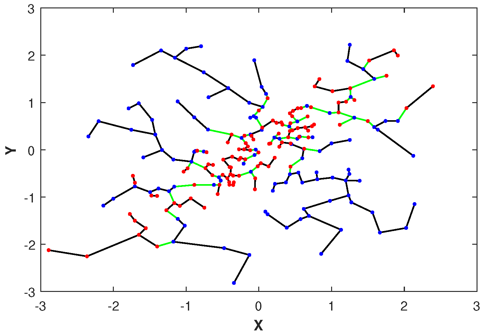
Please note that the asymptotic limit in (11) depends on the proportionality parameter $\alpha$. Later in Section 2.4, we discuss the choice of an optimal parameter $\tilde{\alpha }$. In Figure 1, we illustrate the MST constructed over merged independent ($\rho =0$) and highly dependent ($\rho =0.9$) data sets drawn from two-dimensional normal distributions with correlation coefficients $\rho$. Notice that the edges of the MST connecting samples with different colors, corresponding to independent and dependent samples, respectively, are indicated in green. The total number of green edges is the FR test statistic ${\mathfrak{R}}_{n^{\prime },n^{″}}({\mathcal{Z}}_{n^{\prime }}^{\prime },{\tilde{\mathcal{Z}}}_{n^{″}})$.

2.3. Convergence Rates

In this subsection we characterize the MSE convergence rates of the GMI estimator of Section 2.2 in the form of upper bounds on the bias and the variance. This MSE bound is given in terms of the sample size n, the dimension d, and the proportionality parameter $\alpha$. Deriving convergence rates for mutual information estimators has been of interest in information theory and machine learning [22,27]. The rates are typically derived in terms of a smoothness condition on the densities, such as the Hölder condition [41]. Here we assume $f_X$, $f_Y$ and $f_{XY}$ have support sets ${\mathbb{S}}_X$, ${\mathbb{S}}_Y$, and ${\mathbb{S}}_{XY}:={\mathbb{S}}_X\times {\mathbb{S}}_Y$, respectively, and are smooth in the sense that they belong to Hölder continuous classes of densities ${\mathsf{\Sigma }}_d^s(\eta ,$ K), $0<\eta \le 1$ [42,43]:

Definition 1.

(Hölder class): Let $\mathcal{X}\subset {\mathbb{R}}^d$ be a compact space. The Hölder class of functions ${\mathsf{\Sigma }}_d(\eta ,K)$, with Hölder parameters η and K, consists of functions g that satisfy

$$\begin{array}{c}\left\{g:\parallel g(\mathbf{z})-p_{\mathbf{x}}^{\lfloor \eta \rfloor }(\mathbf{z}){\parallel }_d\le K\parallel \mathbf{x}-\mathbf{z}{\parallel }_d^{\eta },\mathbf{x},\mathbf{z}\in \mathcal{X}\right\},\hfill \end{array}$$

(12)

where $p_{\mathbf{x}}^k(\mathbf{z})$ is the Taylor polynomial (multinomial) of g of order k expanded about the point $\mathbf{x}$ and $\lfloor \eta \rfloor$ is defined as the greatest integer strictly less than η.

To explore the optimal choice of parameter $\alpha$ we require bounds on the bias and variance bounds, provided in Appendix A.5. To obtain such bounds, we will make several assumptions on the absolutely continuous densities $f_X$, $f_Y$, $f_{XY}$ and support sets ${\mathbb{S}}_X$, ${\mathbb{S}}_Y$, ${\mathbb{S}}_{XY}$:

(A.1)

Each of the densities belong to ${\displaystyle {\mathsf{\Sigma }}_d(\eta ,K)}$ with smoothness parameters $\eta$ and Lipschitz constant K.

(A.2)

The volumes of the support sets are finite, i.e., $0<\mathbb{V}({\mathbb{S}}_X)<\infty ,0<\mathbb{V}({\mathbb{S}}_Y)<\infty$.

(A.3)

All densities are bounded i.e., there exist two sets of constants $C_X^L,C_Y^L,C_{XY}^L$ and $C_X^U,C_Y^U,C_{XY}^U$ such that $0<C_X^L\le f_X\le C_X^U<\infty$, $0<C_Y^L\le f_Y\le C_Y^U<\infty$ and $0<C_{XY}^L\le f_{XY}\le C_{XY}^U<\infty$.

The following theorem on the bias follows under assumptions (A.1) and (A.3):

Theorem 4.

For given $\alpha \in (0,1)$, $\beta =1-\alpha$, $d\ge 2$, and $0<\eta \le 1$ the bias of the ${\mathfrak{R}}_{n^{\prime },n^{″}}:={\mathfrak{R}}_{n^{\prime },n^{″}}({\mathcal{Z}}_{n^{\prime }}^{\prime },{\tilde{\mathcal{Z}}}_{n^{″}})$ satisfies

$$\begin{array}{c}{\displaystyle |\frac{\mathbb{E}\left[{\mathfrak{R}}_{n^{\prime },n^{″}}\right]}{n}-2\alpha \beta \int \int \frac{f_{\mathbf{X}\mathbf{Y}}(\mathbf{x},\mathbf{y})f_{\mathbf{X}}(\mathbf{x})f_{\mathbf{Y}}(\mathbf{y})}{\alpha f_{\mathbf{X}\mathbf{Y}}(\mathbf{x},\mathbf{y})+\beta f_{\mathbf{X}}(\mathbf{x})f_{\mathbf{Y}}(\mathbf{y})}\mathrm{d}\mathbf{x}\mathrm{d}\mathbf{y}|}\hfill \\ \le O\left(max\left\{n^{-{\eta }^2/(d(1+\eta ))},{(\beta n)}^{-\eta /(1+\eta )},c_d{n}^{-1}\right\}\right),\hfill \end{array}$$

(13)

where $c_d$ is the largest possible degree of any vertex of MST on ${\mathcal{Z}}_{n^{\prime }}^{\prime }\cup {\tilde{\mathcal{Z}}}_{n^{″}}$. The explicit form of (13) is provided in Appendix A.5.

Please note that according to Theorem 13 in [44], the constant $c_d$ is lower bounded by $\mathsf{\Omega }\left(\sqrt{d}{2}^{n(1-H(\gamma ))}\right)$, $\gamma =2^{-d}$ and $H(\gamma )$ is the binary entropy i.e.,

$$H(\gamma )=-\gamma log\gamma -(1-\gamma )log(1-\gamma ).$$

A proof of Theorem 4 is given in Appendix A.5. The next theorem gives an upper bound on the variance of the FR estimator ${\mathfrak{R}}_{n^{\prime },n^{″}}$. The proof of the variance result requires a different approach than the bias bound (the Efron–Stein inequality [45]). It is similar to arguments in ([46], Appendix A.3), and is omitted. In Theorem 5 we assume that the densities $f_X$, $f_Y$, and $f_{XY}$ are absolutely continuous and bounded (A.3).

Theorem 5.

Given $\alpha \in (0,1)$, the variance of the estimator ${\mathfrak{R}}_{n^{\prime },n^{″}}:={\mathfrak{R}}_{n^{\prime },n^{″}}({\mathcal{Z}}_{n^{\prime }}^{\prime },{\tilde{\mathcal{Z}}}_{n^{″}})$ is bounded by

$${\displaystyle Var\left({\displaystyle \frac{{\mathfrak{R}}_{n^{\prime },n^{″}}}{n}}\right)\le \frac{(1-\alpha )c_d}{n},\alpha =n^{\prime }/n,}$$

(14)

where $c_d$ is a constant depending only on the dimension d.

2.4. Minimax Parameter $\alpha$

Recall assumptions (A.1), (A.2), and (A.3) in Section 2.3. The constant $\alpha$ can be chosen to minimize the maximum the MSE converges rate where the maximum is taken over the space of Hölder smooth joint densities $f_{XY}$.

Throughout this subsection we use the following notations:

• ${ϵ}_{XY}:=f_{XY}/f_X{f}_Y$,
• $C_{ϵ}^L:=C_{XY}^L/C_X^U{C}_Y^U$ and $C_{ϵ}^U:=C_{XY}^U/C_X^L{C}_Y^L$,
• $C_n:=C_{XY}^{L}n/2$,
• ${\displaystyle {\alpha }_0^L:=\frac{2}{C_n}}$ and ${\alpha }_0^U:=min\left\{{\displaystyle \frac{1}{4},\frac{1+1/C_n}{4+2C_{ϵ}^U},1-n^{\eta /d-1}}\right\}$, where $\eta$ is the smoothness parameter,
• $l_n:=⌊n^{\eta /(d^2(1+\eta ))}⌋$.

Now define ${\tilde{G}}_{{ϵ}_{XY},n}^{\alpha ,\beta }(\mathbf{x},\mathbf{y})$ by

$${\displaystyle \frac{({ϵ}_{XY}(\mathbf{x},\mathbf{y})+1/(\beta C_n))(1+{ϵ}_{XY}(\mathbf{x}\mathbf{y})+1/(\beta C_n))}{{(\alpha +\beta {ϵ}_{XY}(\mathbf{x},\mathbf{y}))}^2},\beta =1-\alpha .}$$

(15)

Consider the following optimization problem:

$$\begin{array}{cc}\underset{\alpha }{\min }\underset{{ϵ}_{XY}}{\max }\hfill & \tilde{\Delta }(\alpha ,{ϵ}_{XY})+c_d(1-\alpha )n^{-1}\hfill \\ \mathrm{subject}\mathrm{to}\hfill & C_{ϵ}^L\le {ϵ}_{XY}\le C_{ϵ}^U,\hfill \\ & {\alpha }_0^L\le \alpha \le {\alpha }_0^U,\hfill \end{array}$$

(16)

where

$${\displaystyle \tilde{\Delta }(\alpha ,{ϵ}_{XY}):=D(n,l_n,d,\eta )+\tilde{D}(n,l_n,d)C_{XY}^U{\int \int }_{{\mathbb{S}}_{XY}}{\tilde{G}}_{{ϵ}_{XY},n}^{\alpha ,\beta }(\mathbf{x},\mathbf{y})\mathrm{d}\mathbf{x}\mathrm{d}\mathbf{y},}$$

(17)

and

$$\begin{array}{c}{\displaystyle D(n,l_n,d,\eta )=c_2{l}_n^d{n}^{-1}+c_d{2}^d{n}^{-1}+c^{\prime }{l}_n^d{n}^{-\eta /d}+c{l}_n^d{n}^{-1/d}+2c_1{l}_n^{d-1}{n}^{1/d-1}+c_3{l}_n^{-d\eta },}\hfill \end{array}$$

(18)

$$\begin{array}{c}{\displaystyle \tilde{D}(n,l_n,d)=2+n^{-1}2c^{″}\sum _{i=1}^M{l}_n{l}_n^d{a}_i^{-1}+n^{-3/2}2c_1^{\prime }\sum _{i=1}^M{l}_n{l}_n^{d/2}\sqrt{b_i}{a}_i^2}\hfill \\ {\displaystyle +n^{-1}\sum _{i=1}^{M}2n^{-3/2}{l}_n^{-d/2}\frac{\sqrt{b_i}}{a_i^2}{\left(n{a}_i{l}_n^d+n^2{a}_i^2\right)}^{1/2}{\left(n{b}_i{l}_n^d+n^2{b}_i^2\right)}^{1/2}.}\hfill \end{array}$$

(19)

Please note that in (18), $c,c^{\prime },c_1,c_2$ are constants, and $c_d$ only depends on the dimension d. Also, in (19), $a_i$ and $b_i$ are constants. Let ${ϵ}_{XY}^{*}$ be the optimal ${ϵ}_{XY}$ i.e., ${ϵ}_{XY}^{*}$ be the solution of the optimization problem (16). Set

$$\begin{array}{c}{\displaystyle \mathsf{\Xi }(\alpha ):=\frac{\mathrm{d}}{\mathrm{d}\alpha }\left(\tilde{\Delta }(\alpha ,{ϵ}_{XY}^{*})+c_d(1-\alpha )n^{-1}\right),}\hfill \end{array}$$

(20)

such that ${\displaystyle \tilde{\Delta }(\alpha ,{ϵ}_{XY}^{*})}$ is (17) when ${ϵ}_{XY}={ϵ}_{XY}^{*}$. For $\alpha \in [{\alpha }_0^L,{\alpha }_0^U]$, the optimal choice of ${ϵ}_{XY}$ in terms of maximizing the MSE is ${ϵ}_{XY}^{*}=C_{ϵ}^U$ and the saddle point for the parameter $\alpha$, denoted by $\tilde{\alpha }$, is given as follows:

• $\tilde{\alpha }={\alpha }_0^U$, if $\mathsf{\Xi }({\alpha }_0^U)<0$.
• $\tilde{\alpha }={\alpha }_0^L$, if $\mathsf{\Xi }({\alpha }_0^L)>0$.
• $\tilde{\alpha }={\mathsf{\Xi }}^{-1}(0)$, if ${\alpha }_0^L\le {\mathsf{\Xi }}^{-1}(0)\le {\alpha }_0^U$.

Further details are given in Appendix A.6.

3. Simulation Study

In this section, numerical simulations are presented that illustrate the theory in Section 2. We perform multiple experiments to demonstrate the utility of the proposed GMI estimator of the HP-divergence in terms of the dimension d and the sample size n. Our proposed MST-based estimator of the GMI is compared to density plug-in estimators of the GMI, in particular the standard KDE density plug-in estimator of [22], where the convergence rates of Theorems 4 and 5 are validated. We use multivariate normal simulated data in the experiments. In this section, we also discuss the choice of the proportionality parameter $\alpha$ and compare runtime of the proposed GMI estimator approach with KDE method.

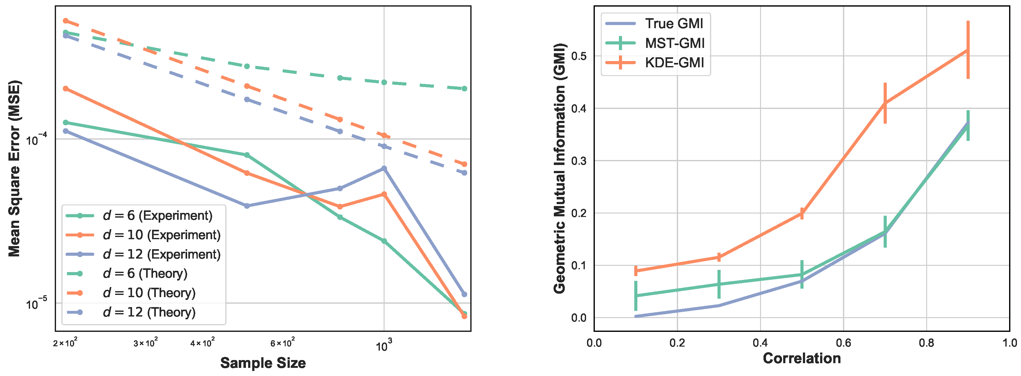
Here we perform four sets of experiments to illustrate the proposed GMI estimator. For the first set of experiments the MSE of the GMI estimator in Algorithm 1 is shown in Figure 2-left. The samples were drawn from d-dimensional normal distribution, with various sample sizes and dimensions $d=6,10,12$. We selected the proportionality parameter $\alpha =0.3$ and computed the MSE in terms of the sample size n. We show the log–log plot of MSE when n varies in $[100,1500]$. Please note that the empirically optimal proportion $\alpha$ depends on n, so to avoid the computational complexity we fixed $\alpha$ for this experiment. The experimental result shown in Figure 2-left validates the theoretical MSE growth rates derived from (13) and (14), i.e., decreasing sub-linearly in n and increasing exponentially in d.

In Figure 2-right, we compare the proposed MST-based GMI estimator with the KDE-GMI estimator [22]. For the KDE approach, we estimated the joint and marginal densities and then plugged them into the proposed expression (2). The bandwidth h used for the KDE plug-in estimator was set as $h=n^{-1/(d+1)}$. The choice of h minimizes the bound on the MSE of the plug-in estimator. We generated data from the two-dimensional normal distribution with zero mean and covariance matrix

$$\left(\begin{array}{cc}1& \rho \\ \rho & 1\end{array}\right).$$

(21)

The coefficient $\rho$ is varied in range $[0.1,0.9]$. The true GMI was computed by the Monte Carlo approximation to the integral (2). Please note that as $\rho$ increases, the MST-GMI outperforms the KDE-GMI approach. In this set of experiments $\alpha =0.6$.

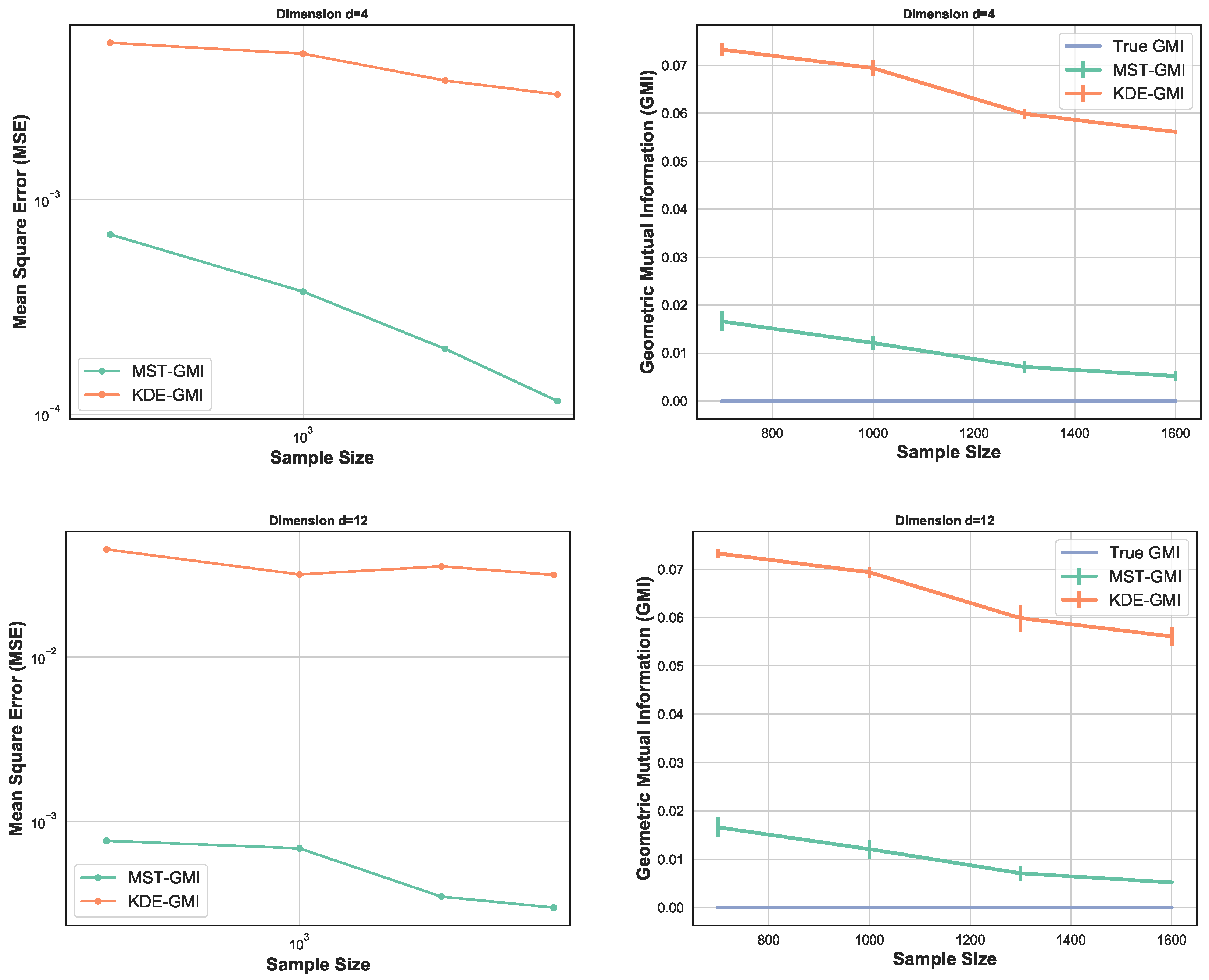
Figure 3 again compares the MST-GMI estimator with the KDE-GMI estimator. samples are drawn from the multivariate standard normal distribution with dimensions $d=4$ and $d=12$. In both cases the proportionality parameter $\alpha =0.5$. The left plots in Figure 3 show the MSE (100 trials) of the GMI estimator implemented with an KDE estimator (with bandwidth as in Figure 2 i.e., $h=n^{-1/(d+1)}$) for dimensions $d=4,12$ and various sample sizes. For all dimensions and sample sizes the MST-GMI estimator also outperforms the plug-in KDE-GMI estimator based on the estimated log–log MSE slope given in Figure 3 (left plots). The right plots in Figure 3 compares the MST-GMI with the KDE-GMI. In this experiment, the error bars denote standard deviations with 100 trials. We observe that for higher dimension $d=12$ and larger sample size n, the KDE-GMI approaches the true GMI at a slower rate than the MST-GMI estimator. This reflects the power of the proposed graph-based approach to estimating GMI.

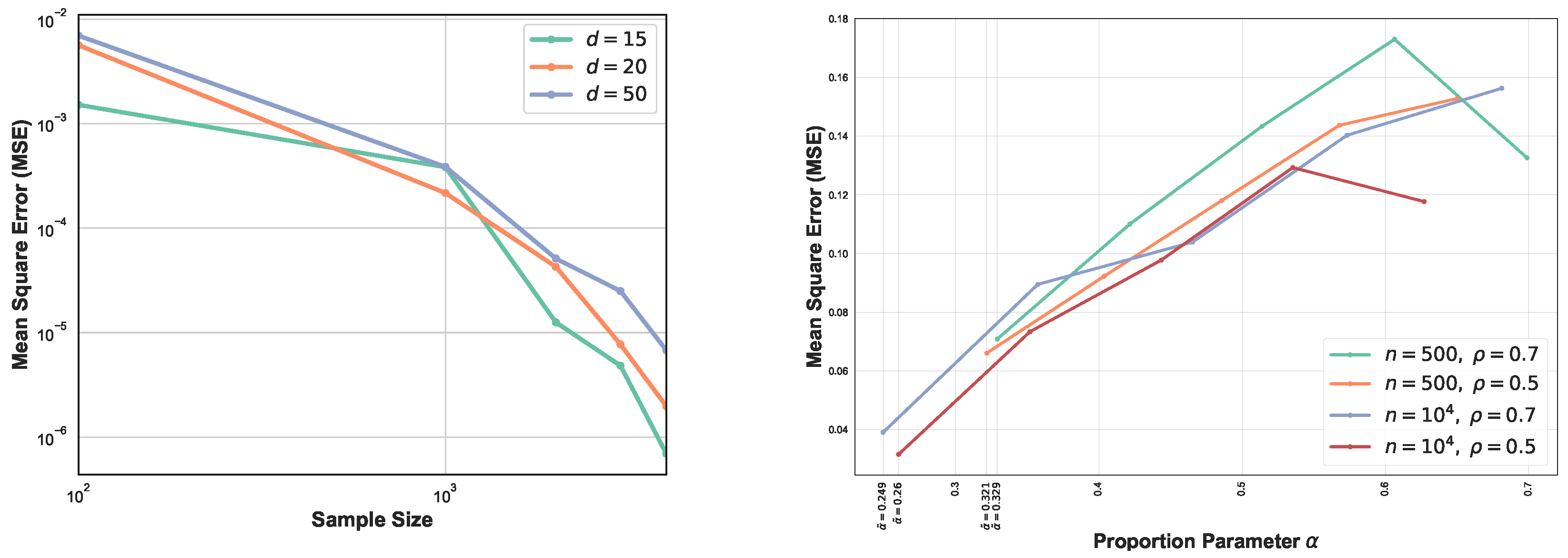
The comparison between MSEs for various dimension d is shown in Figure 4 (left). This experiment highlights the impact of higher dimension on the GMI estimators. As expected, for larger sample size n, MSE decreases while for higher dimension it increases. In this setting, we have generated samples from standard normal distribution with size $n\in [{10}^2,4\times {10}^3]$ and $\alpha =0.5$. From Figure 4 (left) we observe that for larger sample size, MSE curves are ordered based on their corresponding dimensions. Results in Section 2.4 strongly depend on the lower bounds $C_X^L,C_Y^L,C_{XY}^L$ and upper bounds $C_X^U,C_Y^U,C_{XY}^U$ and provide optimal parameter $\alpha$ in the range $[{\alpha }_0^L,{\alpha }_0^U]$, therefore in the experiment section we only analyze one case where the lower bounds $C_X^L,C_Y^L,C_{XY}^L$ and upper bounds $C_X^U,C_Y^U,C_{XY}^U$ are known and the optimal $\alpha$ becomes ${\alpha }_0^L$. Figure 4 (right) illustrates the MSE vs proportion parameter $\alpha$ when $n=500,{10}^4$ samples are generated from truncated normal distribution with $\rho =0.7,0.5$. First, following Section 2.4, we compute the bound $[{\alpha }_0^L,{\alpha }_0^U]$ and then derive the optimal $\alpha$ in this range. Therefore, each experiment with different sample size and $\rho$ provides different range $[{\alpha }_0^L,{\alpha }_0^U]$. We observe that the MSE does not appeared a monotonic function in $\alpha$ and its behavior strongly depends on sample size n, d, and density functions’ bounds. Additional study of the dependency is described in Appendix A.6. In this set of experiments $\mathsf{\Xi }({\alpha }_0^L)>0$, therefore following the results in Section 2.4, we have $\tilde{\alpha }={\alpha }_0^L$. In this experiment the optimal value of $\alpha$ is always the lower bound ${\alpha }_0^L$ and indicated in the Figure 4 (right).

The parameter $\alpha$ is studied further for three scenarios where the lower bounds $C_X^L,C_Y^L,C_{XY}^L$ and upper bounds $C_X^U,C_Y^U,C_{XY}^U$ are assumed unknown, therefore results in Section 2.4 are not applicable. In this set of experiments, we varied $\alpha$ in the range $(0,1)$ to divide our original sample. We generated sample from an isotropic multivariate standard normal distribution $(\rho =0)$ in all three scenarios (all features are independent). Therefore, the true GMI is zero and in all scenarios the GMI column, corresponding to the MST-GMI, is compared with zero. In each scenario we fixed dimension d and sample size n and varied $\alpha =0.2,0.5,0.8$. The dimension and sample size in Scenarios 1,2, and 3 are $d=6,8,10$ and $n=1000,1500,2000$, respectively. In

Table 1. Comparison between different scenarios of various dimensions and sample sizes in terms of parameter $\alpha$. We applied the MST-GMI estimator to estimate the GMI ($I_{\alpha }$) with $\alpha =0.2,0.5,0.8$. We varied dimension $d=6,8,10$ and sample size $n=1000,1500,2000$ in each scenario. We observe that for $\alpha =\{0.2,0.5,0.8\}$, the MST-GMI estimator provides lowest MSE when $\alpha =0.5$ indicated by star (*).

Overview Table for Different d, n, and $\mathit{\alpha }$
Experiments	Dimension ($\mathit{d}$)	Sample Size ($\mathit{n}$)	GMI (${\mathit{I}}_{\mathit{\alpha }}$)	MSE ($\times {\mathbf{10}}^{-\mathbf{4}}$)	Parameter ($\mathit{\alpha }$)
Scenario 1–1	6	1000	0.0229	12	0.2
Scenario 1–2	6	1000	0.0143	4.7944	0.5 *
Scenario 1–3	6	1000	0.0176	6.3867	0.8
Scenario 2–1	8	1500	0.0246	11	0.2
Scenario 2–2	8	1500	0.0074	1.6053	0.5 *
Scenario 2–3	8	1500	0.0137	5.3863	0.8
Scenario 3–1	10	2000	0.0074	2.3604	0.2
Scenario 3–2	10	2000	0.0029	0.54180	0.5 *
Scenario 3–3	10	2000	0.0262	11	0.8

the last column ($\alpha$) stars the parameter $\alpha \in \{0.2,0.5,0.8\}$ with the minimum MSE and GMI $(I_{\alpha })$ in each scenario. Table 1 shows that in these sets of experiments when $\alpha =0.5$, the GMI estimator has less MSE (i.e., is more accurate) than when $\alpha =0.2$ or $\alpha =0.8$. This experimentally demonstrates that if we split our training data, the proposed Algorithm 1 performs better with $\alpha =0.5$.

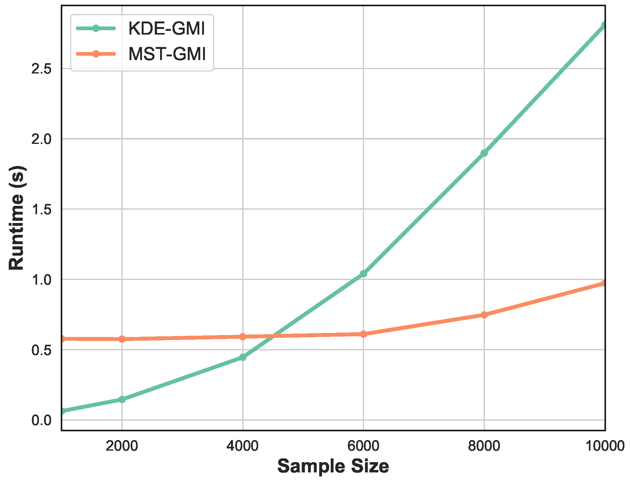
Finally, Figure 5 shows the runtime as a function of sample size n. We vary sample size in the range $[{10}^3,{10}^4]$. Observe that for smaller number of samples the KDE-GMI method is slightly faster but as n becomes large we see significant relative speedup of the proposed MST-GMI method.

4. Conclusions

In this paper, we have proposed a new measure of mutual information, called Geometric MI (GMI), which is related to the Henze–Penrose divergence. The GMI can be viewed as dependency measure that is the limit of the Friedman–Rafsky test statistic, which depends on the MST over all data points. We established some properties of the GMI in terms of convexity/concavity, chain rule, and a type of data-processing inequality. A direct estimator of the GMI, called the MST-GMI, was introduced that uses random permutations of observed relationships between variables in the multivariate samples. An explicit form for the MSE convergence rate bound was derived that depends on a free parameter called the proportionality parameter. An asymptotically optimal form for this free parameter was given that minimizes the MSE convergence rate. Simulation studies were performed that illustrate and verify the theory.

References

- Lewi, J.; Butera, R.; Paninski, L. Real-time adaptive information theoretic optimization of neurophysiology experiments. In Advances in Neural Information Processing Systems; The MIT Press: Cambridge, MA, USA, 2006; pp. 857–864. [Google Scholar]
- Peng, H.C.; Herskovits, E.H.; Davatzikos, C. Bayesian Clustering Methods for Morphological Analysis of MR Images. In Proceedings of the IEEE International Symposium on Biomedical Imaging, Washington, DC, USA, 7–10 July 2002; pp. 485–488. [Google Scholar]
- Moon, K.R.; Noshad, M.; Yasaei Sekeh, S.; Hero, A.O. Information theoretic structure learning with confidence. In Proceedings of the 2017 IEEE International Conference on Acoustics, Speech and Signal Processing (ICASSP), New Orleans, LA, USA, 5–9 March 2017. [Google Scholar]
- Brillinger, D.R. Some data analyses using mutual information. Braz. J. Probab. Stat. 2004, 18, 163–183. [Google Scholar]
- Torkkola, K. Feature extraction by non parametric mutual information maximization. J. Mach. Learn. Res. 2003, 3, 1415–1438. [Google Scholar]
- Vergara, J.R.; Estévez, P.A. A review of feature selection methods based on mutual information. Neural Comput. Appl. 2014, 24, 175–186. [Google Scholar] [CrossRef]
- Peng, H.; Long, F.; Ding, C. Feature selection based on mutual information criteria of max-dependency, max-relevance. IEEE Trans. Pattern Anal. Mach. Intell. 2005, 27, 1226–1238. [Google Scholar] [CrossRef] [PubMed]
- Peng, H.; Long, F.; Ding, C. Evaluation, Application, and Small Sample Performance. IEEE Trans. Pattern Anal. Mach. Intell. 1997, 19, 153–158. [Google Scholar]
- Sorjamaa, A.; Hao, J.; Lendasse, A. Mutual information and knearest neighbors approximator for time series prediction. Lecture Notes Comput. Sci. 2005, 3697, 553–558. [Google Scholar]
- Mohamed, S.; Rezende, D.J. Variational information maximization for intrinsically motivated reinforcement learning. In Advances in Neural Information Processing Systems; The MIT Press: Cambridge, MA, USA, 2015; pp. 2116–2124. [Google Scholar]
- Neemuchwala, H.; Hero, A.O. Entropic graphs for registration. In Multi-Sensor Image Fusion and its Applications; CRC Press Book: Boca Raton, FL, USA, 2005; pp. 185–235. [Google Scholar]
- Neemuchwala, H.; Hero, A.O.; Zabuawala, S.; Carson, P. Image registration methods in high-dimensional space. Int. J. Imaging Syst. Technol. 2006, 16, 130–145. [Google Scholar] [CrossRef] [Green Version]
- Henze, N.; Penrose, M.D. On the multivarite runs test. Ann. Stat. 1999, 27, 290–298. [Google Scholar]
- Berisha, V.; Hero, A.O. Empirical non-parametric estimation of the Fisher information. IEEE Signal Process. Lett. 2015, 22, 988–992. [Google Scholar] [CrossRef]
- Berisha, V.; Wisler, A.; Hero, A.O.; Spanias, A. Empirically estimable classification bounds based on a nonparametric divergence measure. IEEE Trans. Signal Process. 2016, 64, 580–591. [Google Scholar] [CrossRef]
- Kailath, T. The divergence and Bhattacharyya distance measures in signal selection. IEEE Trans. Commun. Technol. 1967, 15, 52–60. [Google Scholar] [CrossRef]
- Yasaei Sekeh, S.; Oselio, B.; Hero, A.O. Multi-class Bayes error estimation with a global minimal spanning tree. In Proceedings of the 2018 56th Annual Allerton Conference on Communication, Control, and Computing (Allerton), Monticello, IL, USA, 2–5 October 2018. [Google Scholar]
- Noshad, M.; Moon, K.R.; Yasaei Sekeh, S.; Hero, A.O. Direct Estimation of Information Divergence Using Nearest Neighbor Ratios. In Proceedings of the IEEE International Symposium on Information Theory (ISIT), Aachen, Germany, 25–30 June 2017. [Google Scholar]
- March, W.; Ram, P.; Gray, A. Fast Euclidean minimum spanning tree: Algorithm, analysis, and applications. In Proceedings of the 16th ACM SIGKDD International Conference on Knowledge Discovery and Data Mining, Boston, MA, USA, 20–23 August 2010; pp. 603–612. [Google Scholar]
- Borůvka, O. O jistém problému minimálním. Práce Moravské Pridovedecké Spolecnosti 1926, 3, 37–58. [Google Scholar]
- Kraskov, A.; Stögbauer, H.; Grassberger, P. Estimating mutual information. Phys. Rev. E 2004, 69, 066–138. [Google Scholar] [CrossRef] [PubMed]
- Moon, K.R.; Sricharan, K.; Hero, A.O. Ensemble Estimation of Mutual Information. In Proceedings of the IEEE International Symposium on Information Theory (ISIT), Aachen, Germany, 25–30 June 2017; pp. 3030–3034. [Google Scholar]
- Moon, K.R.; Hero, A.O. Multivariate f-divergence estimation with confidence. In Proceedings of the Advances in Neural Information Processing Systems 27 (NIPS 2014), Montreal, QC, Canada, 8–13 December 2014; pp. 2420–2428. [Google Scholar]
- Moon, K.R.; Sricharan, K.; Greenewald, K.; Hero, A.O. Improving convergence of divergence functional ensemble estimators. In Proceedings of the IEEE International Symposium on Information Theory (ISIT), Barcelona, Spain, 10–15 July 2016. [Google Scholar]
- Leonenko, N.; Pronzato, L.; Savani, V. A class of Rényi information estimators for multidimensional densities. Ann. Stat. 2008, 36, 2153–2182. [Google Scholar] [CrossRef]
- Gao, S.; Ver Steeg, G.; Galstyan, A. Efficient estimation of mutual information for strongly dependent variables. In Proceedings of the Eighteenth International Conference on Artificial Intelligence and Statistics, San Diego, CA, USA, 9–12 May 2015; pp. 277–286. [Google Scholar]
- Pál, D.; Póczos, B.; Szapesvári, C. Estimation of Rényi entropy and mutual information based on generalized nearest-neighbor graphs. In Proceedings of the 24th Annual Conference on Neural Information Processing Systems 2010, Vancouver, BC, Canada, 6–9 December 2010. [Google Scholar]
- Krishnamurthy, A.; Kandasamy, K.; Póczos, B.; Wasserman, L. Nonparametric estimation of Rényi divergence and friends. In Proceedings of the 31st International Conference on Machine Learning, Beijing, China, 21–26 June 2014; pp. 919–927. [Google Scholar]
- Kandasamy, K.; Krishnamurthy, A.; Póczos, B.; Wasserman, L.; Robins, J. Nonparametric von mises estimators for entropies, divergences and mutual informations. In Proceedings of the Advances in Neural Information Processing Systems, Montreal, QC, Canada, 7–12 December 2015; pp. 397–405. [Google Scholar]
- Singh, S.; Póczos, B. Analysis of k nearest neighbor distances with application to entropy estimation. In Proceedings of the Advances in Neural Information Processing Systems, Barcelona, Spain, 5–10 December 2016; pp. 1217–1225. [Google Scholar]
- Sugiyama, M. Machine learning with squared-loss mutual information. Entropy 2012, 15, 80–112. [Google Scholar] [CrossRef]
- Costa, A.; Hero, A.O. Geodesic entropic graphs for dimension and entropy estimation in manifold learning. IEEE Trans. Signal Process. 2004, 52, 2210–2221. [Google Scholar] [CrossRef]
- Friedman, J.H.; Rafsky, L.C. Multivariate generalizations of the Wald-Wolfowitz and Smirnov two-sample tests. Ann. Stat. 1979, 7, 697–717. [Google Scholar] [CrossRef]
- Smirnov, N.V. On the estimation of the discrepancy between empirical curves of distribution for two independent samples. Bull. Moscow Univ. 1939, 2, 3–6. [Google Scholar]
- Wald, A.; Wolfowitz, J. On a test whether two samples are from the same population. Ann. Math. Stat. 1940, 11, 147–162. [Google Scholar] [CrossRef]
- Noshad, M.; Hero, A.O. Scalable mutual information estimation using dependence graphs. In Proceedings of the International Conference on Artificial Intelligence and Statistics (AISTAT), Brighton, UK, 12–17 May 2019. [Google Scholar]
- Yasaei Sekeh, S.; Oselio, B.; Hero, A.O. A Dimension-Independent discriminant between distributions. In Proceedings of the 2018 IEEE International Conference on Acoustics, Speech and Signal Processing (ICASSP), Calgary, AB, Canada, 15–20 April 2018. [Google Scholar]
- Csiszár, I. Information-type measures of difference of probability distributions and indirect observations. Studia Sci. Math. Hungar. 1967, 2, 299–318. [Google Scholar]
- Ali, S.; Silvey, S.D. A general class of coefficients of divergence of one distribution from another. J. R. Stat. Soc. Ser. B (Methodol.) 1966, 28, 131–142. [Google Scholar] [CrossRef]
- Cover, T.; Thomas, J. Elements of Information Theory, 1st ed.; John Wiley & Sons: Chichester, UK, 1991. [Google Scholar]
- Härdle, W. Applied Nonparametric Regression; Cambridge University Press: Cambridge, UK, 1991. [Google Scholar]
- Lorentz, G.G. Approximation of Functions; Holt, Rinehart and Winston: New York, NY, USA; Chicago, IL, USA; Toronto, ON, Canada, 1966. [Google Scholar]
- Andersson, P. Characterization of pointwise Hölder regularity. Appl. Comput. Harmon. Anal. 1997, 4, 429–443. [Google Scholar] [CrossRef]
- Robins, G.; Salowe, J.S. On the maximum degree of minimum spanning trees. In Proceedings of the SCG 94 Tenth Annual Symposium on Computational Geometry, Stony Brook, NY, USA, 6–8 June 1994; pp. 250–258. [Google Scholar]
- Efron, B.; Stein, C. The jackknife estimate of variance. Ann. Stat. 1981, 9, 586–596. [Google Scholar] [CrossRef]
- Yasaei Sekeh, S.; Noshad, M.; Moon, K.R.; Hero, A.O. Convergence Rates for Empirical Estimation of Binary Classification Bounds. arXiv 2018, arXiv:1810.01015. [Google Scholar]
- Kingman, J.F.C. Poisson Processes; Oxford Univ. Press: Oxford, UK, 1993. [Google Scholar]
- Yukich, J.E. Probability Theory of Classical Euclidean Optimization; Vol. 1675 of Lecture Notes in Mathematics; Springer: Berlin, Germany, 1998. [Google Scholar]
- Luenberger, D.G. Optimization by Vector Space Methods; Wiley Professional Paperback Series; Wiley-Interscience: Hoboken, NJ, USA, 1969. [Google Scholar]
Figure 1.
The MST and FR statistic of spanning the merged set of normal points when and are independent (denoted in blue points) and when and are highly dependent (denoted in red points). The FR test statistic is the number of edges in the MST that connect samples from different color nodes (denoted in green) and it is used to estimate the GMI .
Figure 2.
(left) Log–log plot of theoretical and experimental MSE of the proposed MST-based GMI estimator as a function of sample size n for and fixed smoothness parameter . (right) The GMI estimator was implemented using two approaches, Algorithm 1 and KDE method where the KDE-GMI used KDE density estimators in the formula (2). In this experiment, samples are generated from the two-dimensional normal distribution with zero mean and covariance matrix (21) for various value of .
Figure 3.
MSE log–log plots as a function of sample size n (left) for the proposed MST-GMI estimator (“Estimated GMI”) and the standard KDE-GMI plug-in estimator of GMI. The right column of plots correspond to the GMI estimated for dimension (top) and (bottom). In both cases the proportionality parameter is . The MST-GMI estimator in both plots for sample size n in outperforms the KDE-GMI estimator, especially for larger dimensions.
Figure 4.
MSE log–log plots as a function of sample size n for the proposed FR estimator. We compare the MSE of our proposed FR estimator for various dimensions (left). As d increases, the blue curve takes larger values than green and orange curves i.e., MSE increases as d grows. However, this is more evidential for large sample size n. The second experiment (right) focuses on optimal proportion for and . is the optimal for .
Figure 5.
Runtime of KDE approach and proposed MST-based estimator of GMI vs sample size. The proposed GMI estimator achieves significant speedup, while for small sample size, the KDE method becomes overly fast. Please note that in this experiment the sample is generated from the Gaussian distribution in dimension .