Ensemble Estimation of Information Divergence ^†

Abstract

Recent work has focused on the problem of nonparametric estimation of information divergence functionals between two continuous random variables. Many existing approaches require either restrictive assumptions about the density support set or difficult calculations at the support set boundary which must be known a priori. The mean squared error (MSE) convergence rate of a leave-one-out kernel density plug-in divergence functional estimator for general bounded density support sets is derived where knowledge of the support boundary, and therefore, the boundary correction is not required. The theory of optimally weighted ensemble estimation is generalized to derive a divergence estimator that achieves the parametric rate when the densities are sufficiently smooth. Guidelines for the tuning parameter selection and the asymptotic distribution of this estimator are provided. Based on the theory, an empirical estimator of Rényi-$\alpha$ divergence is proposed that greatly outperforms the standard kernel density plug-in estimator in terms of mean squared error, especially in high dimensions. The estimator is shown to be robust to the choice of tuning parameters. We show extensive simulation results that verify the theoretical results of our paper. Finally, we apply the proposed estimator to estimate the bounds on the Bayes error rate of a cell classification problem.

1. Introduction

Information divergences are integral functionals of two probability distributions and have many applications in the fields of information theory, statistics, signal processing, and machine learning. Some applications of divergences include estimating the decay rates of error probabilities [1], estimating bounds on the Bayes error [2,3,4,5,6,7,8] or the minimax error [9] for a classification problem, extending machine learning algorithms to distributional features [10,11,12,13], testing the hypothesis that two sets of samples come from the same probability distribution [14], clustering [15,16,17], feature selection and classification [18,19,20], blind source separation [21,22], image segmentation [23,24,25], and steganography [26]. For many more applications of divergence measures, see reference [27]. There are many information divergence families including Alpha- and Beta-divergences [28] as well as f-divergences [29,30]. In particular, the f-divergence family includes the well-known Kullback–Leibler (KL) divergence [31], the Rényi-$\alpha$ divergence integral [32], the Hellinger–Bhattacharyya distance [33,34], the Chernoff-$\alpha$ divergence [5], the total variation distance, and the Henze–Penrose divergence [6].

Despite the many applications of divergences between continuous random variables, there are no nonparametric estimators of these functionals that achieve the parametric mean squared error (MSE) convergence rate, are simple to implement, do not require knowledge of the boundary of the density support set, and apply to a large set of divergence functionals. In this paper, we present the first information divergence estimator that achieves all of the above. Specifically, we address the problem of estimating divergence functionals when only a finite population of independent and identically distributed (i.i.d.) samples is available from the two d-dimensional distributions that are unknown, nonparametric, and smooth. Our contributions are as follows:

• We propose the first information divergence estimator, referred to as EnDive, that is based on ensemble methods. The ensemble estimator takes a weighted average of an ensemble of weak kernel density plug-in estimators of divergence where the weights are chosen to improve the MSE convergence rate. This ensemble construction makes it very easy to implement EnDive.
• We prove that the proposed ensemble divergence estimator achieves the optimal parametric MSE rate of $O\left(\frac{1}{N}\right)$, where N is the sample size when the densities are sufficiently smooth. In particular, EnDive achieves these rates without explicitly performing boundary correction which is required for most other estimators. Furthermore, we show that the convergence rates are uniform.
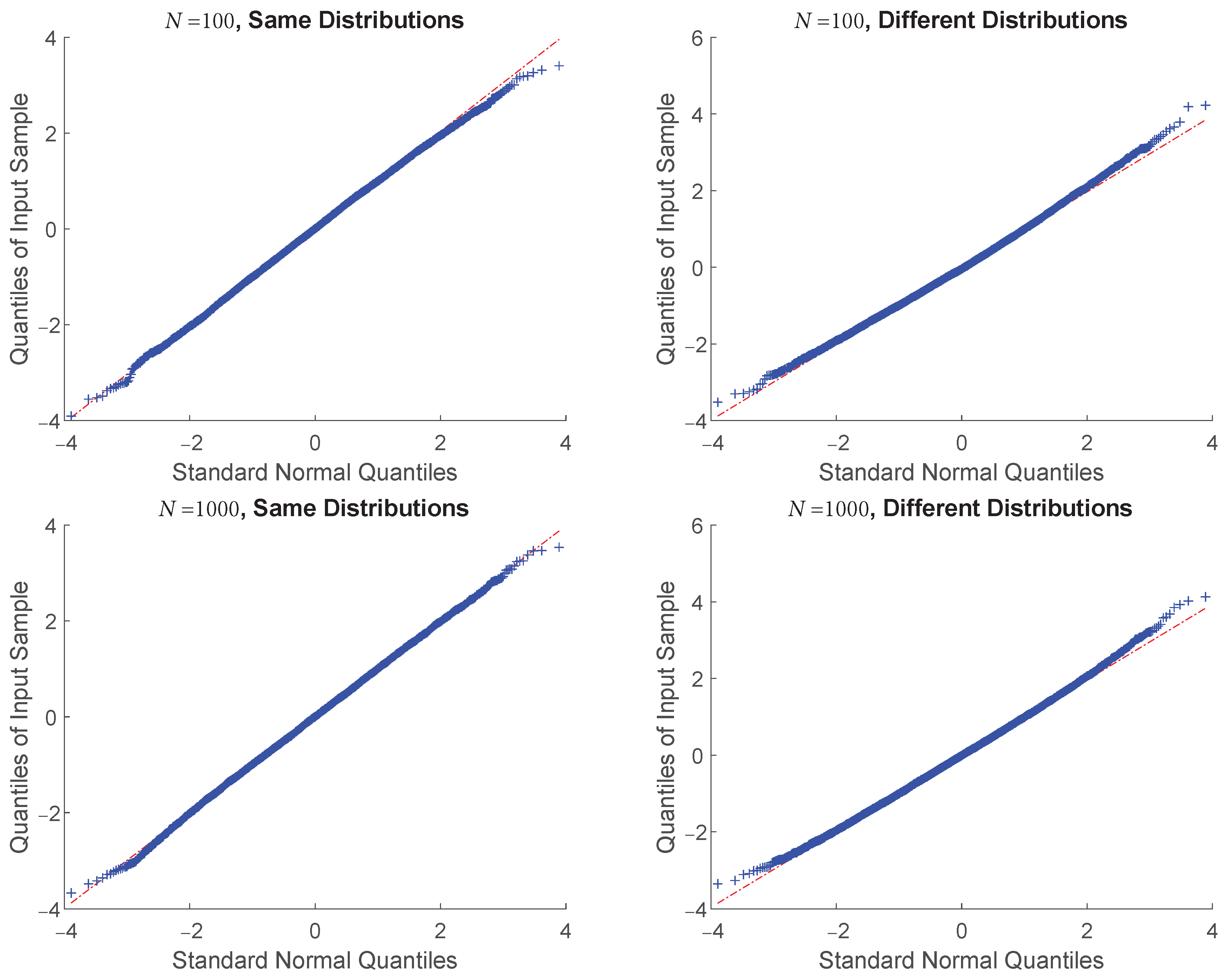
• We prove that EnDive obeys a central limit theorem and thus, can be used to perform inference tasks on the divergence such as testing that two populations have identical distributions or constructing confidence intervals.

1.1. Related Work

Much work has focused on the problem of estimating the entropy and the information divergence of discrete random variables [1,29,35,36,37,38,39,40,41,42,43]. However, the estimation problem for discrete random variables differs significantly from the continuous case and thus employs different tools for both estimation and analysis.

One approach to estimating the differential entropy and information divergence of continuous random variables is to assume a parametric model for the underlying probability distributions [44,45,46]. However, these methods perform poorly when the parametric model does not fit the data well. Unfortunately, the structure of the underlying data distribution is unknown for many applications, and thus the chance for model misspecification is high. Thus, in many of these applications, parametric methods are insufficient, and nonparametric estimators must be used.

While several nonparametric estimators of divergence functionals between continuous random variables have been previously defined, the convergence rates are known for only a few of them. Furthermore, the asymptotic distributions of these estimators are unknown for nearly all of them. For example, Póczos and Schneider [10] established a weak consistency for a bias-corrected k-nearest neighbor (nn) estimator for Rényi-$\alpha$ and other divergences of a similar form where k was fixed. Li et al. [47] examined k-nn estimators of entropy and the KL divergence using hyperspherical data. Wang et al. [48] provided a k-nn based estimator for KL divergence. Plug-in histogram estimators of mutual information and divergence have been proven to be consistent [49,50,51,52]. Hero et al. [53] provided a consistent estimator for Rényi-$\alpha$ divergence when one of the densities is known. However none of these works studied the convergence rates or the asymptotic distribution of their estimators.

There has been recent interest in deriving convergence rates for divergence estimators for continuous data [54,55,56,57,58,59,60]. The rates are typically derived in terms of a smoothness condition on the densities, such as the Hölder condition [61]:

Definition 1 (Hölder Class).

Let $\mathcal{X}\subset {\mathbb{R}}^d$ be a compact space. For $r=(r_1,\dots ,r_d),$ $r_i\in \mathbb{N},$ define $\left|r\right|={\sum }_{i=1}^d{r}_i$ and $D^r=\frac{{\partial }^{\left|r\right|}}{\partial x_1^{r_1}\dots \partial x_d^{r_d}}$. The Hölder class $\mathsf{\Sigma }(s,K_H)$ of functions on $L_2(\mathcal{X})$ consists of the functions (f) that satisfy

$$\left|D^{r}f(x)-D^{r}f(y)\right|\le K_H{∥x-y∥}^{min(s-|r|,1)},$$

for all $x,y\in \mathcal{X}$ and for all r s.t. $\left|r\right|\le ⌊s⌋$.

From Definition 1, it is clear that if a function (f) belongs to $\mathsf{\Sigma }(s,K_H)$, then f is continuously differentiable up to order $⌊s⌋$. In this work, we show that EnDive achieves a parametric MSE convergence rate of $O(1/N)$ when $s\ge d$ and $s>\frac{d}{2}$, depending on the specific form of the divergence function.

Nguyen et al. [56] proposed an f-divergence estimator that estimates the likelihood ratio of the two densities by solving a convex optimization problem and then plugging it into the divergence formulas. The authors proved that the minimax MSE convergence rate is parametric when the likelihood ratio is a member of the bounded Hölder class $\mathsf{\Sigma }(s,K_H)$ with $s\ge d/2$. However, this estimator is restricted to true f-divergences and may not apply to the broader class of divergence functionals that we consider here (as an example, the $L_2^2$ divergence is not an f-divergence). Additionally, solving the convex problem of [56] has similar computational complexity to that of training a support vector machine (SVM) (between $O(N^2)$ and $O(N^3)$), which can be demanding when N is large. In contrast, the EnDive estimator that we propose requires only the construction of simple density plug-in estimates and the solution of an offline convex optimization problem. Therefore, the most computationally demanding step in the EnDive estimator is the calculation of the density estimates, which has a computational complexity no greater than $O(N^2)$.

Singh and Póczos [58,59] provided an estimator for Rényi-$\alpha$ divergences as well as general density functionals that use a “mirror image” kernel density estimator. They proved that these estimators obtain an MSE convergence rate of $O\left(\frac{1}{N}\right)$ when $s\ge d$ for each of the densities. However their approach requires several computations at each boundary of the support of the densities which is difficult to implement as d gets large. Also, this computation requires knowledge of the support (specifically, the boundaries) of the densities which is unknown in most practical settings. In contrast, while our assumptions require the density support sets to be bounded and the boundaries to be smooth, knowledge of the support is not required to implement EnDive.

The “linear” and “quadratic” estimators presented by Krishnamurthy et al. [57] estimate divergence functionals that include the form $\int f_1^{\alpha }(x)f_2^{\beta }(x)d\mu (x)$ for given $\alpha$ and $\beta$ where $f_1$ and $f_2$ are probability densities. These estimators achieve the parametric rate when $s\ge d/2$ and $s\ge d/4$ for the linear and quadratic estimators, respectively. However, the latter estimator is computationally infeasible for most functionals, and the former requires numerical integration for some divergence functionals which can be computationally difficult. Additionally, while a suitable $\alpha$-$\beta$ indexed sequence of divergence functionals of this form can be constructed that converge to the KL divergence, this does not guarantee convergence of the corresponding sequence of divergence estimators, as shown in reference [57]. In contrast, EnDive can be used to estimate the KL divergence directly. Other important f-divergence functionals are also excluded from this form including some that bound the Bayes error [2,4,6]. In contrast, our method applies to a large class of divergence functionals and avoids numerical integration.

Finally, Kandasamy et al. [60] proposed influence function-based estimators of distributional functionals including divergences that achieve the parametric rate when $s\ge d/2$. While this method can be applied to general functionals, the estimator requires numerical integration for some functionals. Additionally, the estimators in both Kandasamy et al. [60] and Krishnamurthy et al. [57] require an optimal kernel density estimator. This is difficult to construct when the density support is bounded as it requires difficult computations at the density support set boundary and therefore, knowledge of the density support set. In contrast, Endive does not require knowledge of the support boundary.

In addition to the MSE convergence rates, the asymptotic distribution of divergence estimators is of interest. Asymptotic normality has been established for certain divergences between a specific density estimator and the true density [62,63,64]. This differs from the problem we consider where we assume that both densities are unknown. The asymptotic distributions of the estimators in references [56,57,58,59] are currently unknown. Thus, it is difficult to use these estimators for hypothesis testing which is crucial in many scientific applications. Kandasamy et al. [60] derived the asymptotic distribution of their data-splitting estimator but did not prove similar results for their leave-one-out estimator. We establish a central limit theorem for EnDive which greatly enhances its applicability in scientific settings.

Our ensemble divergence estimator reduces to an ensemble entropy estimator as a special case when data from only one distribution is considered and the other density is set to a uniform measure (see reference [28] for more on the relationship between entropy and information divergence). The resultant entropy estimator differs from the ensemble entropy estimator proposed by Sricharan et al. [65] in several important ways. First, the density support set must be known for the estimator in reference [65] to perform the explicit boundary correction. In contrast, the EnDive estimator does not require any boundary correction. To show this requires a significantly different approach to prove the bias and variance rates of the EnDive estimator. Furthermore, the EnDive results apply under more general assumptions for the densities and the kernel used in the weak estimators. Finally, the central limit theorem applies to the EnDive estimator which is currently unknown for the estimator in reference [65].

We also note that Berrett et al. [66] proposed a modification of the Kozachenko and Leonenko estimator of entropy [67] that takes a weighted ensemble estimation approach. While their results require stronger assumptions for the smoothness of the densities than ours do, they did obtain the asymptotic distribution of their weighted estimator and they also showed that the asymptotic variance of the estimator is not increased by taking a weighted average. This latter point is an important selling point of the ensemble framework—we can improve the asymptotic bias of an estimator without increasing the asymptotic variance.

1.2. Organization and Notation

The paper is organized as follows. We first derive the MSE convergence rates in Section 2 for a weak divergence estimator, which is a kernel density plug-in divergence estimator. We then generalize the theory of optimally weighted ensemble entropy estimation developed in reference [65] to obtain the ensemble divergence estimator EnDive from an ensemble of weak estimators in Section 3. A central limit theorem and uniform convergence rate for the ensemble estimator are also presented in Section 3. In Section 4, we provide guidelines for selecting the tuning parameters based on experiments and the theory derived in the previous sections. We then perform experiments in Section 4 that validate the theory and establish the robustness of the proposed estimators to the tuning parameters.

Bold face type is used for random variables and random vectors. The conditional expectation given a random variable $\mathbf{Z}$ is denoted as ${\mathbb{E}}_{\mathbf{Z}}$. The variance of a random variable is denoted as $\mathbb{V}$, and the bias of an estimator is denoted as $\mathbb{B}$.

2. The Divergence Functional Weak Estimator

This paper focuses on estimating functionals of the form

$$G\left(f_1,f_2\right)=\int g\left(f_1(x),f_2(x)\right)f_2(x)dx,,$$

(1)

where $g(x,y)$ is a smooth functional, and $f_1$ and $f_2$ are smooth d-dimensional probability densities. If $g\left(f_1(x),f_2(x)\right)=g\left(\frac{f_1(x)}{f_2(x)}\right),$ g is convex, and $g(1)=0$, then $G\left(f_1,f_2\right)$ defines the family of f-divergences. Some common divergences that belong to this family include the KL divergence ($g(t)=-lnt$) and the total variation distance ($g(t)=|t-1|$). In this work, we consider a broader class of functionals than the f-divergences, since g is allowed to be very general.

To estimate $G\left(f_1,f_2\right)$, we first define a weak plug-in estimator based on kernel density estimators (KDEs), that is, a simple estimator that converges slowly to the true value $G\left(f_1,f_2\right)$ in terms of MSE. We then derive the bias and variance expressions for this weak estimator as a function of sample size and bandwidth. We then use the resulting bias and variance expressions to derive an ensemble estimator that takes a weighted average of weak estimators with different bandwidths and achieves superior MSE performance.

2.1. The Kernel Density Plug-in Estimator

We use a kernel density plug-in estimator of the divergence functional in (1) as the weak estimator. Assume that $N_1$ i.i.d. realizations $\left\{{\mathbf{Y}}_1,\dots ,{\mathbf{Y}}_{N_1}\right\}$ are available from $f_1$ and $N_2$ i.i.d. realizations $\left\{{\mathbf{X}}_1,\dots ,{\mathbf{X}}_{N_2}\right\}$ are available from $f_2$. Let $h_i>0$ be the kernel bandwidth for the density estimator of $f_i$. For simplicity of presentation, assume that $N_1=N_2=N$ and $h_1=h_2=h$. The results for the more general case of differing sample sizes and bandwidths are given in Appendix C. Let $K(·)$ be a kernel function with $\int K(x)dx=1$ and ${\left|\right|K\left|\right|}_{\infty }<\infty$ where ${\parallel K\parallel }_{\infty }$ is the ${\ell }_{\infty }$ norm of the kernel (K). The KDEs for $f_1$ and $f_2$ are, respectively,

$$\begin{array}{ccc}\hfill {\tilde{\mathbf{f}}}_{1,h}({\mathbf{X}}_j)& =& \frac{1}{N{h}^d}{\displaystyle \sum _{i=1}^N}K\left(\frac{{\mathbf{X}}_j-{\mathbf{Y}}_i}{h}\right),\hfill \\ \hfill {\tilde{\mathbf{f}}}_{2,h}({\mathbf{X}}_j)& =& \frac{1}{M{h}^d}{\displaystyle \sum _{\begin{array}{c}i=1\\ i\ne j\end{array}}^N}K\left(\frac{{\mathbf{X}}_j-{\mathbf{X}}_i}{h}\right),\hfill \end{array}$$

where $M=N-1$. $G\left(f_1,f_2\right)$ is then approximated as

$${\tilde{\mathbf{G}}}_h=\frac{1}{N}{\displaystyle \sum _{i=1}^N}g\left({\tilde{\mathbf{f}}}_{1,h}\left({\mathbf{X}}_i\right),{\tilde{\mathbf{f}}}_{2,h}\left({\mathbf{X}}_i\right)\right).$$

(2)

2.2. Convergence Rates

For many estimators, MSE convergence rates are typically provided in the form of upper (or sometimes lower) bounds on the bias and the variance. Therefore, only the slowest converging terms (as a function of the sample size (N)) are presented in these cases. However, to apply our generalized ensemble theory to obtain estimators that guarantee the parametric MSE rate, we required explicit expressions for the bias of the weak estimators in terms of the sample size (N) and the kernel bandwidth (h). Thus, an upper bound was insufficient for our work. Furthermore, to guarantee the parametric rate, we required explicit expressions of all bias terms that converge to zero slower than $O\left(1/\sqrt{N}\right)$.

To obtain bias expressions, we required multiple assumptions on the densities $f_1$ and $f_2$, the functional g, and the kernel K. Similar to reference [7,54,65], the principal assumptions we make were that (1) $f_1$, $f_2,$ and g are smooth; (2) $f_1$ and $f_2$ have common bounded support sets $\mathcal{S}$; and (3) $f_1$ and $f_2$ are strictly lower bounded on $\mathcal{S}$. We also assume (4) that the density support set is smooth with respect to the kernel ($K(u)$). The full technical assumptions and a discussion of them are contained in Appendix A. Given these assumptions, we have the following result on the bias of ${\tilde{\mathbf{G}}}_h$:

Theorem 1.

For a general g, the bias of the plug-in estimator ${\tilde{\mathbf{G}}}_h$ is given by

$$\mathbb{B}\left[{\tilde{\mathbf{G}}}_h\right]={\displaystyle \sum _{j=1}^{⌊s⌋}}{c}_{10,j}{h}^j+c_{11}\frac{1}{N{h}^d}+O\left(h^s+\frac{1}{N{h}^d}\right).$$

(3)

To apply our generalized ensemble theory to the KDE plug-in estimator (${\tilde{\mathbf{G}}}_h$), we required only an upper bound on its variance. The following variance result required much less strict assumptions than the bias results in Theorem 1:

Theorem 2.

Assume that the functional g in (1) is Lipschitz continuous in both of its arguments with the Lipschitz constant ($C_g$). Then, the variance of the plug-in estimator (${\tilde{\mathbf{G}}}_h$) is bounded by

$$\mathbb{V}\left[{\tilde{\mathbf{G}}}_h\right]\le C_g^2{\left|\right|K\left|\right|}_{\infty }^2\frac{11}{N}.$$

From Theorems 1 and 2, we observe that $h\to 0$ and $N{h}^d\to \infty$ are required for ${\tilde{\mathbf{G}}}_h$ to be unbiased, while the variance of the plug-in estimator depends primarily on the sample size (N). Note that the constants depend on the densities $f_1$ and $f_2$ and their derivatives which are often unknown.

2.3. Optimal MSE Rate

From Theorem 1, the dominating terms in the bias are observed to be $\mathsf{\Theta }\left(h\right)$ and $\mathsf{\Theta }\left(\frac{1}{N{h}^d}\right)$. If no bias correction is performed, the optimal choice of h that minimizes MSE is

$$h^{\ast }=\mathsf{\Theta }\left(N^{\frac{-1}{d+1}}\right).$$

This results in a dominant bias term of order $\mathsf{\Theta }\left(N^{\frac{-1}{d+1}}\right)$. Note that this differs from the standard result for the optimal KDE bandwidth for minimum MSE density estimation which is $\mathsf{\Theta }\left(N^{-1/\left(d+4\right)}\right)$ for a symmetric uniform kernel when the boundary bias is ignored [68].

Figure 1 shows a heatmap showing the leading bias term $O\left(h\right)$ as a function of d and N when $h=N^{\frac{-1}{d+1}}$. The heatmap indicates that the bias of the plug-in estimator in (2) is small only for relatively small values of d. This is consistent with the empirical results in reference [69] which examined the MSE of multiple plug-in KDE and k-nn estimators. In the next section, we propose an ensemble estimator that achieves a superior convergence rate regardless of the dimensions (d) as long as the density is sufficiently smooth.

2.4. Proof Sketches of Theorems 1 and 2

To prove the bias expressions in Theorem 1, the bias is first decomposed into two parts by adding and subtracting $g\left({\mathbb{E}}_{\mathbf{Z}}{\tilde{\mathbf{f}}}_{1,h}(\mathbf{Z}),{\mathbb{E}}_{\mathbf{Z}}{\tilde{\mathbf{f}}}_{2,h}(\mathbf{Z})\right)$ within the expectation creating a “bias” term and a “variance” term. Applying a Taylor series expansion on the bias and variance terms results in expressions that depend on powers of ${\mathbb{B}}_{\mathbf{Z}}\left[{\tilde{\mathbf{f}}}_{i,h}(\mathbf{Z})\right]:={\mathbb{E}}_{\mathbf{Z}}{\tilde{\mathbf{f}}}_{i,h}(\mathbf{Z})-f_i(\mathbf{Z})$ and ${\tilde{\mathbf{e}}}_{i,h}(\mathbf{Z}):={\tilde{\mathbf{f}}}_{i,h}(\mathbf{Z})-{\mathbb{E}}_{\mathbf{Z}}{\tilde{\mathbf{f}}}_{i,h}(\mathbf{Z})$, respectively. Within the interior of the support, moment bounds can be derived from properties of the KDEs and a Taylor series expansion of the densities. Near the boundary of the support, the smoothness assumption on the boundary $\mathcal{A}.5$ is required to obtain an expression of the bias in terms of the KDE bandwidth (h) and the sample size (N). The full proof of Theorem 1 is given in Appendix E.

The proof of the variance result takes a different approach. The proof uses the Efron–Stein inequality [70] which bounds the variance by analyzing the expected squared difference between the plug-in estimator when one sample is allowed to differ. This approach provides a bound on the variance under much less strict assumptions on the densities and the functional g than is required for Theorem 1. The full proof of Theorem 2 is given in Appendix F.

3. Weighted Ensemble Estimation

From Theorem 1 and Figure 1, we can observe that the bias of the MSE-optimal plug-in estimator ${\tilde{\mathbf{G}}}_h$ decreases very slowly as a function of the sample size (N) when the data dimensions (d) are not small, resulting in a large MSE. However, by applying the theory of optimally weighted ensemble estimation, we can obtain an estimator with improved performance by taking a weighted sum of an ensemble of weak estimators where the weights are chosen to significantly reduce the bias.

The ensemble of weak estimators is formed by choosing different values of the bandwidth parameter h as follows. Set $\mathcal{L}=\left\{l_1,\dots ,l_L\right\}$ to be real positive numbers that index $h(l_i)$. Thus, the parameter l indexes over different neighborhood sizes for the KDEs. Define the weight $w:=\left\{w\left(l_1\right),\dots ,w\left(l_L\right)\right\}$ and ${\tilde{\mathbf{G}}}_w:={\sum }_{l\in \mathcal{L}}w(l){\tilde{\mathbf{G}}}_{h(l)}.$ That is, for each estimator ${\tilde{\mathbf{G}}}_{h(l)}$ there is a corresponding weight value ($w(l)$). The key to reducing the MSE is to choose the weight vector (w) to reduce the lower order terms in the bias while minimizing the impact of the weighted average on the variance.

3.1. Finding the Optimal Weight

The theory of optimally weighted ensemble estimation is a general theory that is applicable to any estimation problem as long as the bias and variance of the estimator can be expressed in a specific way. An early version of this theory was presented in reference [65]. We now generalize this theory so that it can be applied to a wider variety of estimation problems. Let N be the number of available samples and let $\mathcal{L}=\left\{l_1,\dots ,l_L\right\}$ be a set of index values. Given an indexed ensemble of estimators ${\left\{{\widehat{\mathbf{E}}}_l\right\}}_{l\in \mathcal{L}}$ of some parameter (E), the weighted ensemble estimator with weights $w=\left\{w\left(l_1\right),\dots ,w\left(l_L\right)\right\}$ satisfying ${\sum }_{l\in \mathcal{L}}w(l)=1$ is defined as

$${\widehat{\mathbf{E}}}_w={\displaystyle \sum _{l\in \mathcal{L}}}w\left(l\right){\widehat{\mathbf{E}}}_l.$$

${\widehat{\mathbf{E}}}_w$ is asymptotically unbiased as long as the estimators ${\left\{{\widehat{\mathbf{E}}}_l\right\}}_{l\in \mathcal{L}}$ are asymptotically unbiased. Consider the following conditions on ${\left\{{\widehat{\mathbf{E}}}_l\right\}}_{l\in \mathcal{L}}$:

• $\mathcal{C}.1$ The bias is expressible as

  $$\mathbb{B}\left[{\widehat{\mathbf{E}}}_l\right]={\displaystyle \sum _{i\in J}}{c}_i{\psi }_i(l){\varphi }_{i,d}(N)+O\left(\frac{1}{\sqrt{N}}\right),$$

  where $c_i$ are constants that depend on the underlying density and are independent of N and l, $J=\left\{i_1,\dots ,i_I\right\}$ is a finite index set with $I<L$, and ${\psi }_i(l)$ are basis functions depending only on parameter l and not on the sample size (N).
• $\mathcal{C}.2$ The variance is expressible as

  $$\mathbb{V}\left[{\widehat{\mathbf{E}}}_l\right]=c_v\left(\frac{1}{N}\right)+o\left(\frac{1}{N}\right).$$

Theorem 3.

Assume conditions $\mathcal{C}.1$ and $\mathcal{C}.2$ hold for an ensemble of estimators ${\left\{{\widehat{\mathbf{E}}}_l\right\}}_{l\in \mathcal{L}}$. Then, there exists a weight vector ($w_0$) such that the MSE of the weighted ensemble estimator attains the parametric rate of convergence:

$$\mathbb{E}\left[{\left({\widehat{\mathbf{E}}}_{w_0}-E\right)}^2\right]=O\left(\frac{1}{N}\right).$$

The weight vector ($w_0$) is the solution to the following convex optimization problem:

$$\begin{array}{cc}\hfill {\displaystyle \underset{w}{min}}& {\left|\right|w\left|\right|}_2\hfill \\ \hfill subjectto& {\displaystyle {\sum }_{l\in \mathcal{L}}}w(l)=1,\hfill \\ & {\gamma }_w(i)={\displaystyle {\sum }_{l\in \mathcal{L}}}w(l){\psi }_i(l)=0,i\in J.\hfill \end{array}$$

(4)

Proof. 

From condition $\mathcal{C}.1$, we can write the bias of the weighted estimator as

$$\mathbb{B}\left[{\widehat{\mathbf{E}}}_w\right]={\displaystyle \sum _{i\in J}}{c}_i{\gamma }_w(i){\varphi }_{i,d}(N)+O\left(\frac{\sqrt{L}{\left|\right|w\left|\right|}_2}{\sqrt{N}}\right).$$

The variance of the weighted estimator is bounded as

$$\mathbb{V}\left[{\widehat{\mathbf{E}}}_w\right]\le \frac{{L\left|\right|w\left|\right|}_2^2}{N}.$$

(5)

The optimization problem in (4) zeroes out the lower-order bias terms and limits the ${\ell }_2$ norm of the weight vector (w) to prevent the variance from exploding. This results in an MSE rate of $O(1/N)$ when the dimensions (d) are fixed and when L is fixed independently of the sample size (N). Furthermore, a solution to (4) is guaranteed to exist if $L>I$ and the vectors $a_i=\left[{\psi }_i(l_1),\dots ,{\psi }_i(l_L)\right]$ are linearly independent. This completes our sketch of the proof of Theorem 3. ☐

3.2. The EnDive Estimator

The parametric rate of $O\left(1/N\right)$ in MSE convergence can be achieved without requiring ${\gamma }_w(i)=0,i\in J$. This can be accomplished by solving the following convex optimization problem in place of the optimization problem in Theorem 3:

$$\begin{array}{cc}\hfill {\displaystyle \underset{w}{min}}& ϵ\hfill \\ \hfill subjectto& {\sum }_{l\in \mathcal{L}}w(l)=1,\hfill \\ & \left|{\gamma }_w(i)N^{\frac{1}{2}}{\varphi }_{i,d}(N)\right|\le ϵ,i\in J,\hfill \\ & {∥w∥}_2^2\le \eta ϵ,\hfill \end{array}$$

(6)

where the parameter $\eta$ is chosen to achieve a trade-off between bias and variance. Instead of forcing ${\gamma }_w(i)=0$, the relaxed optimization problem uses the weights to decrease the bias terms at a rate of $O\left(1/\sqrt{N}\right)$, yielding an MSE convergence rate of $O(1/N).$ In fact, it was shown in reference [71] that the optimization problem in (6) guarantees the parametric MSE rate as long as the conditions of Theorem 3 are satisfied and a solution to the optimization problem in (4) exists (the conditions for this existence are given in the proof of Theorem 3).

We now construct a divergence ensemble estimator from an ensemble of plug-in KDE divergence estimators. Consider first the bias result in (3) where g is general, and assume that $s\ge d$. In this case, the bias contains a $O\left(\frac{1}{h^{d}N}\right)$ term. To guarantee the parametric MSE rate, any remaining lower-order bias terms in the ensemble estimator must be no slower than $O\left(1/\sqrt{N}\right)$. Let $h(l)=l{N}^{-1/(2d)}$ where $l\in \mathcal{L}$. Then $O\left(\frac{1}{h{(l)}^{d}N}\right)=O\left(\frac{1}{l^d\sqrt{N}}\right)$. We therefore obtain an ensemble of plug-in estimators ${\left\{{\tilde{\mathbf{G}}}_{h(l)}\right\}}_{l\in \mathcal{L}}$ and a weighted ensemble estimator ${\tilde{\mathbf{G}}}_w={\sum }_{l\in \mathcal{L}}w(l){\tilde{\mathbf{G}}}_{h(l)}$. The bias of each estimator in the ensemble satisfies the condition $\mathcal{C}.1$ with ${\psi }_i(l)=l^i$ and ${\varphi }_{i,d}(N)=N^{-i/(2d)}$ for $i=1,\dots ,d$. To obtain a uniform bound on the bias with respect to w and $\mathcal{L}$, we also include the function ${\psi }_{d+1}(l)=l^{-d}$ with corresponding ${\varphi }_{d+1,d}(N)=N^{-1/2}$. The variance also satisfies the condition $\mathcal{C}.2$. The optimal weight ($w_0$) is found by using (6) to obtain an optimally weighted plug-in divergence functional estimator ${\tilde{\mathbf{G}}}_{w_0}$ with an MSE convergence rate of $O\left(\frac{1}{N}\right)$ as long as $s\ge d$ and $L\ge d$. Otherwise, if $s<d$, we can only guarantee the MSE rate up to $O\left(\frac{1}{N^{s/d}}\right)$. We refer to this estimator as the Ensemble Divergence (EnDive) estimator and denote it as ${\tilde{\mathbf{G}}}_{\mathrm{EnDive}}$.

We note that for some functionals (g) (including the KL divergence and the Renyi-$\alpha$ divergence integral), we can modify the EnDive estimator to obtain the parametric rate under the less strict assumption that $s>d/2$. For details on this approach, see Appendix B.

3.3. Central Limit Theorem

The following theorem shows that an appropriately normalized ensemble estimator ${\tilde{\mathbf{G}}}_w$ converges in distribution to a normal random variable under rather general conditions. Thus, the same result applies to the EnDive estimator ${\tilde{\mathbf{G}}}_{\mathrm{EnDive}}$. This enables us to perform hypothesis testing on the divergence functional which is very useful in many scientific applications. The proof is based on the Efron–Stein inequality and an application of Slutsky’s Theorem (Appendix G).

Theorem 4.

Assume that the functional g is Lipschitz in both arguments with the Lipschitz constant $C_g$. Further assume that $h(l)=o(1)$, $N\to \infty$, and $Nh{(l)}^d\to \infty$ for each $l\in \mathcal{L}$. Then, for a fixed $\mathcal{L}$, the asymptotic distribution of the weighted ensemble estimator ${\tilde{\mathbf{G}}}_w$ is

$$Pr\left(\left({\tilde{\mathbf{G}}}_w-\mathbb{E}\left[{\tilde{\mathbf{G}}}_w\right]\right)/\sqrt{\mathbb{V}\left[{\tilde{\mathbf{G}}}_w\right]}\le t\right)\to Pr(\mathbf{S}\le t),$$

where $\mathbf{S}$ is a standard normal random variable.

3.4. Uniform Convergence Rates

Here, we show that the optimally weighted ensemble estimators achieve the parametric MSE convergence rate uniformly. Denote the subset of $\mathsf{\Sigma }\left(s,K_H\right)$ with densities bounded between ${ϵ}_0$ and ${ϵ}_{\infty }$ as $\mathsf{\Sigma }\left(s,K_H,{ϵ}_0,{ϵ}_{\infty }\right)$.

Theorem 5.

Let ${\tilde{\mathbf{G}}}_{\mathrm{EnDive}}$ be the EnDive estimator of the functional

$$G(p,q)=\int g\left(p(x),q(x)\right)q(x)dx,$$

where p and q are d-dimensional probability densities. Additionally, let $r=d$ and assume that $s>r$. Then,

$${\displaystyle \underset{p,q\in \mathsf{\Sigma }\left(s,K_H,{ϵ}_0,{ϵ}_{\infty }\right)}{sup}}\mathbb{E}\left[{\left({\tilde{\mathbf{G}}}_{w_0}-G(p,q)\right)}^2\right]\le \frac{C}{N},$$

(7)

where C is a constant.

The proof decomposes the MSE into the variance plus the square of the bias. The variance is bounded easily by using Theorem 2. To bound the bias, we show that the constants in the bias terms are continuous with respect to the densities p and q under an appropriate norm. We then show that $\mathsf{\Sigma }\left(s,K_H,{ϵ}_0,{ϵ}_{\infty }\right)$ is compact with respect to this norm and then apply an extreme value theorem. Details are given in Appendix H.

4. Experimental Results

In this section, we discuss the choice of tuning parameters and validate the EnDive estimator’s convergence rates and the central limit theorem. We then use the EnDive estimator to estimate bounds on the Bayes error for a single-cell bone marrow data classification problem.

4.1. Tuning Parameter Selection

The optimization problem in (6) has parameters $\eta$, L, and $\mathcal{L}$. By applying (6), and the resulting MSE of the ensemble estimator is

$$O\left({ϵ}^2/N\right)+O\left(L{\eta }^2{ϵ}^2/N\right),$$

(8)

where each term in the sum comes from the bias and variance, respectively. From this expression and (6), we see that the parameter $\eta$ provides a tradeoff between bias and variance. Increasing $\eta$ enables the norm of the weight vector to be larger. This means the feasible region for the variable w increases in size as $\eta$ increases which can result in decreased bias. However, as $\eta$ contributes to the variance term, increasing $\eta$ may result in increased variance.

If all of the constants in (3) and an exact expression for the variance of the ensemble estimator were known, then $\eta$ could be chosen to optimize this tradeoff in bias and variance and thus minimize the MSE. Since these constants are unknown, we can only choose $\eta$ based on the asymptotic results. From (8), this would suggest setting $\eta =1/\sqrt{L}$. In practice, we find that for finite sample sizes, the variance in the ensemble estimator is less than the upper bound of $L{\eta }^2{ϵ}^2/N$. Thus, setting $\eta =1/\sqrt{L}$ is unnecessarily restrictive. We find that, in practice, setting $\eta =1$ works well.

Upon first glance, it appears that for fixed L, the set $\mathcal{L}$ that parameterizes the kernel widths can, in theory, be chosen by minimizing $ϵ$ in (6) over $\mathcal{L}$ in addition to w. However, adding this constraint results in a non-convex optimization problem since w does not lie in the non-negative orthant. A parameter search over possible values for $\mathcal{L}$ is another possibility. However, this may not be practical as $ϵ$ generally decreases as the size and spread of $\mathcal{L}$ increases. In addition, for finite sample sizes, decreasing $ϵ$ does not always directly correspond to a decrease in MSE, as very high or very low values of $h(l)$ can lead to inaccurate density estimates, resulting in a larger MSE.

Given these limitations, we provide the following recommendations for $\mathcal{L}$. Denote the value of the minimum value of l such that ${\tilde{\mathbf{f}}}_{i,h(l_{min})}({\mathbf{X}}_j)>0$$\forall i=1,2$ as $l_{min}$ and the diameter of the support $\mathcal{S}$ as D. To ensure the KDEs are bounded away from zero, we require that $min(\mathcal{L})\ge l_{min}$. As demonstrated in Figure 2, the weights in $w_0$ are generally largest for the smallest values of $\mathcal{L}$. This indicates that $min(\mathcal{L})$ should also be sufficiently larger than $l_{min}$ to render an adequate density estimate. Similarly, $max(\mathcal{L})$ should be sufficiently smaller than the diamter (D) as high bandwidth values can lead to high bias in the KDEs. Once these values are chosen, all other $\mathcal{L}$ values can then be chosen to be equally spaced between $min(\mathcal{L})$ and $max(\mathcal{L})$.

An efficient way to choose $l_{min}$ and $l_{max}$ is to select the integers $k_{min}$ and $k_{max}$ and compute the $k_{min}$ and $k_{max}$ nearest neighbor distances of all the data points. The bandwidths $h(l_{min})$ and $h(l_{max})$ can then be chosen to be the maximums of these corresponding distances. The parameters $l_{min}$ and $l_{max}$ can then be computed from the expression $h(l)=l{N}^{-\frac{1}{2d}}$. This choice ensures that a minimum of $k_{min}$ points are within the kernel bandwidth for the density estimates at all points and that a maximum of $k_{max}$ points are within the kernel bandwidth for the density estimates at one of the points.

Once $min(\mathcal{L})$ and $max(\mathcal{L})$ have been chosen, the similarity of bandwidth values $h(l)$ and basis functions ${\psi }_{i,d}(l)$ increases as L increases, resulting in a negligible decrease in the bias. Hence, L should be chosen to be large enough for sufficient bias but small enough so that the bandwidth values $h(l)$ are sufficiently distinct. In our experiments, we found $30\le L\le 60$ to be sufficient.

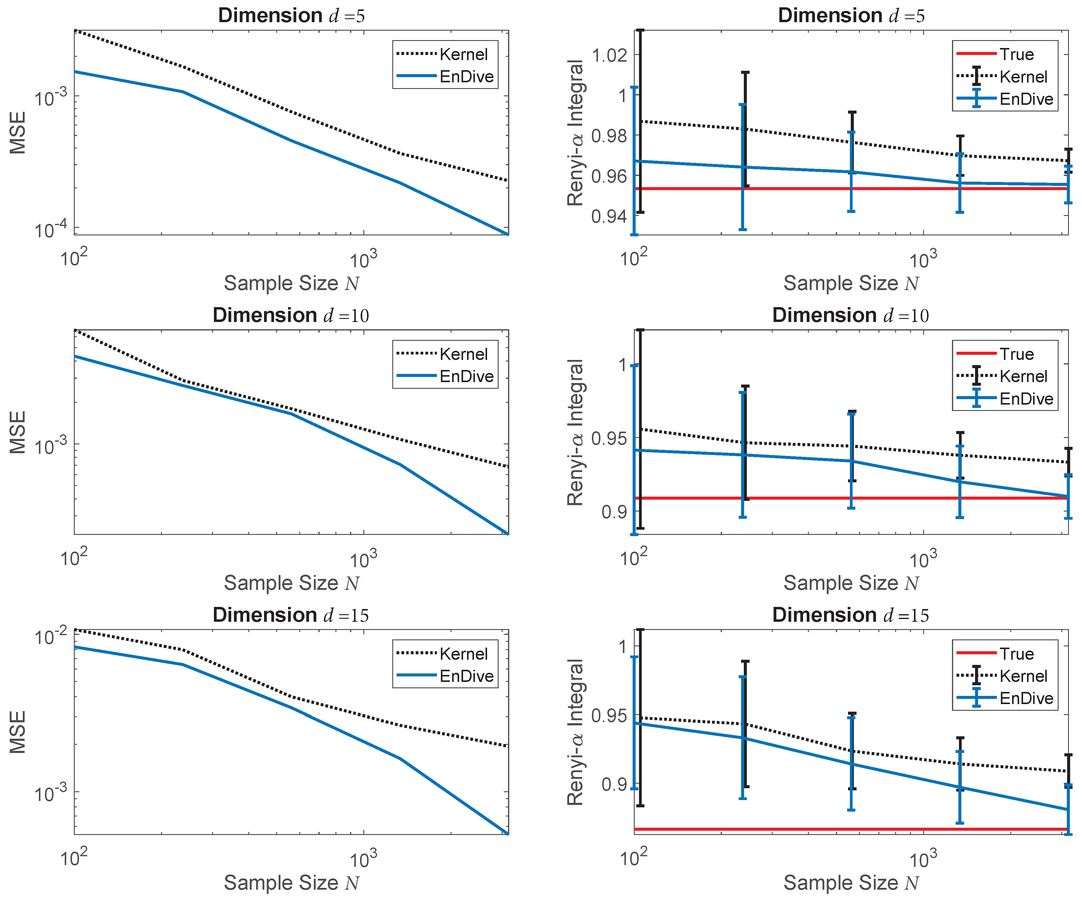
4.2. Convergence Rates Validation: Rényi-$\alpha$ Divergence

To validate our theoretical convergence rate results, we estimated the Rényi-$\alpha$ divergence integral between two truncated multivariate Gaussian distributions with varying dimension and sample sizes. The densities had means of ${\overline{\mu }}_1=0.7\times {\overline{1}}_d$, ${\overline{\mu }}_2=0.3\times {\overline{1}}_d$ and covariance matrices of $0.4\times I_d$, where ${\overline{1}}_d$ is a d-dimensional vector of ones, and $I_d$ is a $d\times d$ identity matrix. We restricted the Gaussians to the unit cube and used $\alpha =0.5$.

The left plots in Figure 3 show the MSE (200 trials) of the standard plug-in estimator implemented with a uniform kernel and the proposed optimally weighted estimator EnDive for various dimensions and sample sizes. The parameter set $\mathcal{L}$ was selected based on a range of k-nearest neighbor distances. The bandwidth used for the standard plug-in estimator was selected by setting $h_{fixed}(l^{\ast })=l^{\ast }{N}^{-\frac{1}{d+1}}$, where $l^{\ast }$ was chosen from $\mathcal{L}$ to minimize the MSE of the plug-in estimator. For all dimensions and sample sizes, EnDive outperformed the plug-in estimator in terms of MSE. EnDive was also less biased than the plug-in estimator and even had lower variance at smaller sample sizes (e.g., $N=100$). This reflects the strength of ensemble estimators—the weighted sum of a set of relatively poor estimators can result in a very good estimator. Note also that for the larger values of N, the ensemble estimator MSE rates approached the theoretical rate based on the estimated log–log slope given in

Table 1. Negative log–log slope of the EnDive mean squared error (MSE) as a function of the sample size for various dimensions. The slope was calculated beginning at $N_{start}$. The negative slope was closer to 1 with $N_{start}={10}^{2.375}$ than for $N_{start}={10}^2$ indicating that the asymptotic rate had not yet taken effect at $N_{start}={10}^2$.

Estimator	$\mathit{d}=5$	$\mathit{d}=10$	$\mathit{d}=15$
$N_{start}={10}^2$	$0.85$	$0.84$	$0.80$
$N_{start}={10}^{2.375}$	$0.96$	$0.96$	$0.95$

.

To illustrate the difference between the problems of density estimation and divergence functional estimation, we estimated the average pointwise squared error between the KDE ${\tilde{\mathbf{f}}}_{1,h}$ and $f_1$ in the previous experiment. We used exactly the same bandwidth and kernel as the standard plug-in estimators in Figure 3 and calculated the pointwise error at 10,000 points sampled from $f_1$. The results are shown in Figure 4. From these results, we see that the KDEs performed worse as the dimension of the densities increased. Additionally, we observe by comparing Figure 3 and Figure 4, the average pointwise squared error decreased at a much slower rate as a function of the sample size (N) than the MSE of the plug-in divergence estimators, especially for larger dimensions (d).

Our experiments indicated that the proposed ensemble estimator is not sensitive to the tuning parameters. See reference [72] for more details.

4.3. Central Limit Theorem Validation: KL Divergence

To verify the central limit theorem of the EnDive estimator, we estimated the KL divergence between two truncated Gaussian densities, again restricted to the unit cube. We conducted two experiments where (1) the densities were different with means of ${\overline{\mu }}_1=0.7\times {\overline{1}}_d$, ${\overline{\mu }}_2=0.3\times {\overline{1}}_d$ and covariances of matrices ${\sigma }_i\times I_d$, ${\sigma }_1=0.1$, ${\sigma }_2=0.3$; and where (2) the densities were the same with means of $0.3\times {\overline{1}}_d$ and covariance matrices of $0.3\times I_d$. For both experiments, we chose $d=6$ and four different sample sizes (N). We found that the correspondence between the quantiles of the standard normal distribution and the quantiles of the centered and scaled EnDive estimator was very high under all settings (see

Table 2. Comparison between quantiles of a standard normal random variable and the quantiles of the centered and scaled EnDive estimator applied to the KL divergence when the distributions were the same and different. Quantiles were computed from 10,000 trials. The parameter $\rho$ gives the correlation coefficient between the quantiles, while $\beta$ is the estimated slope between the quantiles. The correspondence between quantiles was very high for all cases.

N	Same		Different
	$\mathbf{1}\mathbf{-}\mathit{\rho }$	$\mathit{\beta }$	$\mathbf{1}\mathbf{-}\mathit{\rho }$	$\mathit{\beta }$
100	$2.35\times {10}^{-4}$	$1.014$	$9.97\times {10}^{-4}$	$0.993$
500	$9.48\times {10}^{-5}$	$1.007$	$5.06\times {10}^{-4}$	$0.999$
1000	$8.27\times {10}^{-5}$	$0.996$	$4.30\times {10}^{-4}$	$0.988$
5000	$8.59\times {10}^{-5}$	$0.995$	$4.47\times {10}^{-4}$	$1.005$

and Figure 5) which validates Theorem 4.

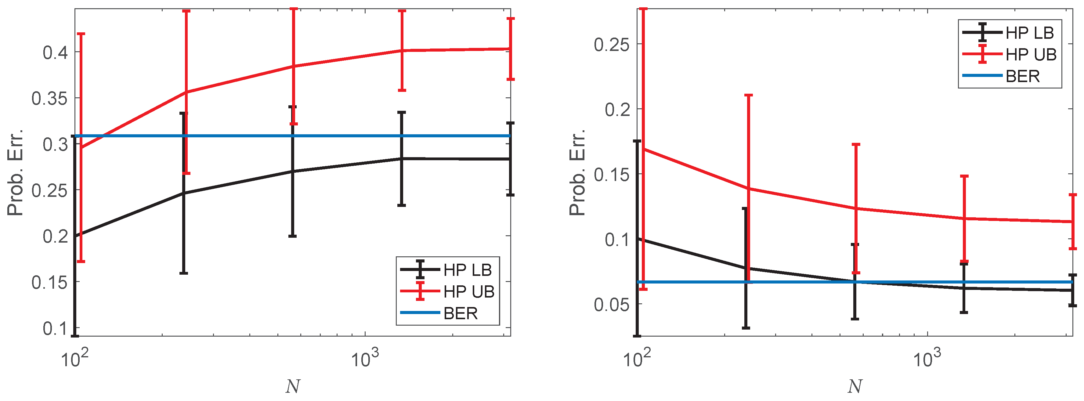
4.4. Bayes Error Rate Estimation on Single-Cell Data

Using the EnDive estimator, we estimated bounds on the Bayes error rate (BER) of a classification problem involving MARS-seq single-cell RNA-sequencing (scRNA-seq) data measured from developing mouse bone marrow cells enriched for the myeloid and erythroid lineages [73]. However, we first demonstrated the ability of EnDive to estimate the bounds on the BER of a simulated problem. In this simulation, the data were drawn from two classes where each class distribution was a $d=10$ dimensional Gaussian distribution with different means and the identity covariance matrix. We considered two cases, namely, the distance between the means was 1 or 3. The BER was calculated in both cases. We then estimated upper and lower bounds on the BER by estimating the Henze–Penrose (HP) divergence [4,6]. Figure 6 shows the average estimated upper and lower bounds on the BER with standard error bars for both cases. For all tested sample sizes, the BER was within one standard deviation of the estimated lower bound. The lower bound was also closer, on average, to the BER for most of the tested sample sizes (lower sample sizes with smaller distances between means were the exceptions). Generally, these resuls indicate that the true BER is relatively close to the estimated lower bound, on average.

We then estimated similar bounds on the scRNA-seq classification problem using EnDive. We considered the three most common cell types within the data: erythrocytes (eryth.), monocytes (mono.), and basophils (baso.) ($N=1095,559,300,$ respectively). We estimated the upper and lower bounds on the pairwise BER between these classes using different combinations of genes selected from the Kyoto Encyclopedia of Genes and Genomes (KEGG) pathways associated with the hematopoietic cell lineage [74,75,76]. Each collection of genes contained 11–14 genes. The upper and lower bounds on the BER were estimated using the Henze–Penrose divergence [4,6]. The standard deviations of the bounds for the KEGG-based genes were estimated via 1000 bootstrap iterations. The KEGG-based bounds were compared to BER bounds obtained from 1000 random selections of 12 genes. In all cases, we compared the bounds to the performance of a quadratic discriminant analysis classifier (QDA) with 10-fold cross validation. Note that to correct for undersampling in scRNA-seq data, we first imputed the undersampled data using MAGIC [77].

All results are given in

Table 3. Misclassification rate of a quadratic discriminant analysis classifier (QDA) classifier and estimated upper bounds (UB) and lower bounds (LB) of the pairwise BER between mouse bone marrow cell types using the Henze–Penrose divergence applied to different combinations of genes selected from the KEGG pathways associated with the hematopoietic cell lineage. Results are presented as percentages in the form of mean ± standard deviation. Based on these results, erythrocytes are relatively easy to distinguish from the other two cell types using these gene sets.

	Platelets	Erythrocytes	Neutrophils	Macrophages	Random
Eryth. vs. Mono., LB	$2.8\pm 1.5$	$1.2\pm 0.6$	$0.6\pm 0.6$	$8.5\pm 1.2$	$14.4\pm 8.4$
Eryth. vs. Mono., UB	$5.3\pm 2.9$	$2.4\pm 1.3$	$1.2\pm 1.3$	$15.5\pm 1.9$	$23.2\pm 12.3$
Eryth. vs. Mono., Prob. Error	$0.9$	$0.4$	$1.3$	$3.4$	$7.2\pm 5.4$
Eryth. vs. Baso., LB	$0.5\pm 0.6$	$0.05\pm 0.12$	$0.6\pm 0.5$	$5.1\pm 0.9$	$11.9\pm 5.5$
Eryth. vs. Baso., UB	$1.0\pm 1.1$	$0.1\pm 0.2$	$1.1\pm 0.9$	$9.6\pm 1.6$	$20.3\pm 8.8$
Eryth. vs. Baso., Prob. Error	$1.2$	$0.3$	$1.9$	$3.6$	$6.8\pm 5.0$
Baso. vs. Mono., LB	$31.1\pm 1.8$	$27.8\pm 3.1$	$27.1\pm 2.6$	$31.6\pm 1.3$	$32.1\pm 2.6$
Baso. vs. Mono., UB	$42.8\pm 1.4$	$39.9\pm 2.8$	$39.4\pm 2.4$	$43.2\pm 1.0$	$43.5\pm 1.2$
Baso. vs. Mono., Prob. Error	$28.8$	$30.9$	$23.9$	$22.4$	$29.7\pm 5.7$

. From these results, we note that erythrocytes are relatively easy to distinguish from the other two cell types as the BER lower bounds were within nearly two standard deviations of zero when using genes associated with platelet, erythrocyte, and neutrophil development as well as a random selection of 12 genes. This is corroborated by the QDA cross-validated results which were all within two standard deviations of either the upper or lower bound for these gene sets. In contrast, the macrophage-associated genes seem to be less useful for distinguishing erythrocytes than the other gene sets.

We also found that basophils are difficult to distinguish from monocytes using these gene sets. Assuming the relative abundance of each cell type is representative of the population, a trivial upper bound on the BER is $300/(300+559)\approx 0.35$ which is between all of the estimated lower and upper bounds. The QDA results were also relatively high (and may be overfitting the data in some cases based on the estimated BER bounds), suggesting that different genes should be explored for this classification problem.

5. Conclusions

We derived the MSE convergence rates for a kernel density plug-in estimator for a large class of divergence functionals. We generalized the theory of optimally weighted ensemble estimation and derived an ensemble divergence estimator EnDive that achieves the parametric rate when the densities are more than d times differentiable. The estimator we derived can be applied to general bounded density support sets and can be implemented without knowledge of the support, which is a distinct advantage over other competing estimators. We also derived the asymptotic distribution of the estimator, provided some guidelines for tuning parameter selection, and experimentally validated the theoretical convergence rates for the case of empirical estimation of the Rényi-$\alpha$ divergence integral. We then performed experiments to examine the estimator’s robustness to the choice of tuning parameters, validated the central limit theorem for KL divergence estimation, and estimated bounds on the Bayes error rate for a single cell classification problem.

We note that based on the proof techniques employed in our work, our weighted ensemble estimators are easily extended beyond divergence estimation to more general distributional functionals which may be integral functionals of any number of probability distributions. We also show in Appendix B that EnDive can be easily modified to obtain an estimator that achieves the parametric rate when the densities are more than $d/2$ times differentiable and the functional g has a specific form that includes the Rényi and KL divergences. Future work includes extending this modification to functionals with more general forms. An important divergence of interest in this context is the Henze–Penrose divergence that we used to bound the Bayes error. Further future work will focus on extending this work on divergence estimation to k-nn based estimators where knowledge of the support is, again, not required. This will improve the computational burden, as k-nn estimators require fewer computations than standard KDEs.

References

1. Cover, T.M.; Thomas, J.A. Elements of Information Theory; John Wiley & Sons: New York, NY, USA, 2012. [Google Scholar]
2. Avi-Itzhak, H.; Diep, T. Arbitrarily tight upper and lower bounds on the Bayesian probability of error. IEEE Trans. Pattern Anal. Mach. Intell. 1996, 18, 89–91. [Google Scholar] [CrossRef]
3. Hashlamoun, W.A.; Varshney, P.K.; Samarasooriya, V. A tight upper bound on the Bayesian probability of error. IEEE Trans. Pattern Anal. Mach. Intell. 1994, 16, 220–224. [Google Scholar] [CrossRef]
4. Moon, K.; Delouille, V.; Hero, A.O., III. Meta learning of bounds on the Bayes classifier error. In Proceedings of the 2015 IEEE Signal Processing and Signal Processing Education Workshop (SP/SPE), Salt Lake City, UT, USA, 9–12 August 2015; pp. 13–18. [Google Scholar]
5. Chernoff, H. A measure of asymptotic efficiency for tests of a hypothesis based on the sum of observations. Ann. Math. Stat. 1952, 23, 493–507. [Google Scholar] [CrossRef]
6. Berisha, V.; Wisler, A.; Hero, A.O., III; Spanias, A. Empirically Estimable Classification Bounds Based on a New Divergence Measure. IEEE Trans. Signal Process. 2016, 64, 580–591. [Google Scholar] [CrossRef] [PubMed]
7. Moon, K.R.; Hero, A.O., III. Multivariate f-Divergence Estimation With Confidence. In Proceedings of the 27th International Conference on Neural Information Processing Systems (NIPS 2014), Montreal, QC, Canada, 8–13 December 2014; pp. 2420–2428. [Google Scholar]
8. Gliske, S.V.; Moon, K.R.; Stacey, W.C.; Hero, A.O., III. The intrinsic value of HFO features as a biomarker of epileptic activity. In Proceedings of the 2016 IEEE International Conference on Acoustics, Speech and Signal Processing (ICASSP), Shanghai, China, 20–25 March 2016. [Google Scholar]
9. Loh, P.-L. On Lower Bounds for Statistical Learning Theory. Entropy 2017, 19, 617. [Google Scholar] [CrossRef]
10. Póczos, B.; Schneider, J.G. On the estimation of alpha-divergences. In Proceedings of the 22nd International Conference on Artificial Intelligence and Statistics, Fort Lauderdale, FL, USA, 11–13 April 2011; pp. 609–617. [Google Scholar]
11. Oliva, J.; Póczos, B.; Schneider, J. Distribution to distribution regression. In Proceedings of the 30th International Conference on Machine Learning, Atlanta, GA, USA, 16–21 June 2013; pp. 1049–1057. [Google Scholar]
12. Szabó, Z.; Gretton, A.; Póczos, B.; Sriperumbudur, B. Two-stage sampled learning theory on distributions. In Proceeding of The 18th International Conference on Artificial Intelligence and Statistics, San Diego, CA, USA, 9–12 May 2015. [Google Scholar]
13. Moon, K.R.; Delouille, V.; Li, J.J.; De Visscher, R.; Watson, F.; Hero, A.O., III. Image patch analysis of sunspots and active regions. II. Clustering via matrix factorization. J. Space Weather Space Clim. 2016, 6, A3. [Google Scholar] [CrossRef]
14. Moon, K.R.; Li, J.J.; Delouille, V.; De Visscher, R.; Watson, F.; Hero, A.O., III. Image patch analysis of sunspots and active regions. I. Intrinsic dimension and correlation analysis. J. Space Weather Space Clim. 2016, 6, A2. [Google Scholar] [CrossRef]
15. Dhillon, I.S.; Mallela, S.; Kumar, R. A divisive information theoretic feature clustering algorithm for text classification. J. Mach. Learn. Res. 2003, 3, 1265–1287. [Google Scholar]
16. Banerjee, A.; Merugu, S.; Dhillon, I.S.; Ghosh, J. Clustering with Bregman divergences. J. Mach. Learn. Res. 2005, 6, 1705–1749. [Google Scholar]
17. Lewi, J.; Butera, R.; Paninski, L. Real-time adaptive information-theoretic optimization of neurophysiology experiments. In Proceedings of the 19th International Conference on Neural Information Processing Systems (NIPS 2006), Vancouver, BC, Canada, 4–9 December 2006; pp. 857–864. [Google Scholar]
18. Bruzzone, L.; Roli, F.; Serpico, S.B. An extension of the Jeffreys-Matusita distance to multiclass cases for feature selection. IEEE Trans. Geosci. Remote Sens. 1995, 33, 1318–1321. [Google Scholar] [CrossRef]
19. Guorong, X.; Peiqi, C.; Minhui, W. Bhattacharyya distance feature selection. In Proceedings of the 13th International Conference on Pattern Recognition, Vienna, Austria, 25–29 August 1996; Volume 2, pp. 195–199. [Google Scholar]
20. Sakate, D.M.; Kashid, D.N. Variable selection via penalized minimum φ-divergence estimation in logistic regression. J. Appl. Stat. 2014, 41, 1233–1246. [Google Scholar] [CrossRef]
21. Hild, K.E.; Erdogmus, D.; Principe, J.C. Blind source separation using Renyi’s mutual information. IEEE Signal Process. Lett. 2001, 8, 174–176. [Google Scholar] [CrossRef]
22. Mihoko, M.; Eguchi, S. Robust blind source separation by beta divergence. Neural Comput. 2002, 14, 1859–1886. [Google Scholar] [CrossRef] [PubMed]
23. Vemuri, B.C.; Liu, M.; Amari, S.; Nielsen, F. Total Bregman divergence and its applications to DTI analysis. IEEE Trans. Med. Imaging 2011, 30, 475–483. [Google Scholar] [CrossRef] [PubMed]
24. Hamza, A.B.; Krim, H. Image registration and segmentation by maximizing the Jensen-Rényi divergence. In Proceedings of the 4th International Workshop Energy Minimization Methods in Computer Vision and Pattern Recognition (EMMCVPR 2003), Lisbon, Portugal, 7–9 July 2003; pp. 147–163. [Google Scholar]
25. Liu, G.; Xia, G.; Yang, W.; Xue, N. SAR image segmentation via non-local active contours. In Proceedings of the 2014 IEEE International Geoscience and Remote Sensing Symposium (IGARSS), Quebec City, QC, Canada, 13–18 July 2014; pp. 3730–3733. [Google Scholar]
26. Korzhik, V.; Fedyanin, I. Steganographic applications of the nearest-neighbor approach to Kullback-Leibler divergence estimation. In Proceedings of the 2015 Third International Conference on Digital Information, Networking, and Wireless Communications (DINWC), Moscow, Russia, 3–5 February 2015; pp. 133–138. [Google Scholar]
27. Basseville, M. Divergence measures for statistical data processing–An annotated bibliography. Signal Process. 2013, 93, 621–633. [Google Scholar] [CrossRef]
28. Cichocki, A.; Amari, S. Families of alpha-beta-and gamma-divergences: Flexible and robust measures of similarities. Entropy 2010, 12, 1532–1568. [Google Scholar] [CrossRef]
29. Csiszar, I. Information-type measures of difference of probability distributions and indirect observations. Stud. Sci. Math. Hungar. 1967, 2, 299–318. [Google Scholar]
30. Ali, S.M.; Silvey, S.D. A general class of coefficients of divergence of one distribution from another. J. R. Stat. Soc. Ser. B Stat. Methodol. 1966, 28, 131–142. [Google Scholar]
31. Kullback, S.; Leibler, R.A. On information and sufficiency. Ann. Math. Stat. 1951, 22, 79–86. [Google Scholar] [CrossRef]
32. Rényi, A. On measures of entropy and information. In Proceedings of the Fourth Berkeley Symposium on Mathematical Statistics and Probability, Berkeley, CA, USA, 20 June–30 July 1960; University of California Press: Berkeley, CA, USA, 1961; pp. 547–561. [Google Scholar]
33. Hellinger, E. Neue Begründung der Theorie quadratischer Formen von unendlichvielen Veränderlichen. J. Rein. Angew. Math. 1909, 136, 210–271. (In German) [Google Scholar]
34. Bhattacharyya, A. On a measure of divergence between two multinomial populations. Indian J. Stat. 1946, 7, 401–406. [Google Scholar]
35. Silva, J.F.; Parada, P.A. Shannon entropy convergence results in the countable infinite case. In Proceedings of the 2012 IEEE International Symposium on Information Theory Proceedings (ISIT), Cambridge, MA, USA, 1–6 July 2012; pp. 155–159. [Google Scholar]
36. Antos, A.; Kontoyiannis, I. Convergence properties of functional estimates for discrete distributions. Random Struct. Algorithms 2001, 19, 163–193. [Google Scholar] [CrossRef]
37. Valiant, G.; Valiant, P. Estimating the unseen: An n/log (n)-sample estimator for entropy and support size, shown optimal via new CLTs. In Proceedings of the 43rd Annual ACM Symposium on Theory of Computing, San Jose, CA, USA, 6–8 June 2011; pp. 685–694. [Google Scholar]
38. Jiao, J.; Venkat, K.; Han, Y.; Weissman, T. Minimax estimation of functionals of discrete distributions. IEEE Trans. Inf. Theory 2015, 61, 2835–2885. [Google Scholar] [CrossRef] [PubMed]
39. Jiao, J.; Venkat, K.; Han, Y.; Weissman, T. Maximum likelihood estimation of functionals of discrete distributions. IEEE Trans. Inf. Theory 2017, 63, 6774–6798. [Google Scholar] [CrossRef]
40. Valiant, G.; Valiant, P. The power of linear estimators. In Proceedings of the 2011 IEEE 52nd Annual Symposium on Foundations of Computer Science (FOCS), Palm Springs, CA, USA, 22–25 October 2011; pp. 403–412. [Google Scholar]
41. Paninski, L. Estimation of entropy and mutual information. Neural Comput. 2003, 15, 1191–1253. [Google Scholar] [CrossRef]
42. Paninski, L. Estimating entropy on m bins given fewer than m samples. IEEE Trans. Inf. Theory 2004, 50, 2200–2203. [Google Scholar] [CrossRef]
43. Alba-Fernández, M.V.; Jiménez-Gamero, M.D.; Ariza-López, F.J. Minimum Penalized ϕ-Divergence Estimation under Model Misspecification. Entropy 2018, 20, 329. [Google Scholar] [CrossRef]
44. Ahmed, N.A.; Gokhale, D. Entropy expressions and their estimators for multivariate distributions. IEEE Trans. Inf. Theory 1989, 35, 688–692. [Google Scholar] [CrossRef]
45. Misra, N.; Singh, H.; Demchuk, E. Estimation of the entropy of a multivariate normal distribution. J. Multivar. Anal. 2005, 92, 324–342. [Google Scholar] [CrossRef]
46. Gupta, M.; Srivastava, S. Parametric Bayesian estimation of differential entropy and relative entropy. Entropy 2010, 12, 818–843. [Google Scholar] [CrossRef]
47. Li, S.; Mnatsakanov, R.M.; Andrew, M.E. K-nearest neighbor based consistent entropy estimation for hyperspherical distributions. Entropy 2011, 13, 650–667. [Google Scholar] [CrossRef]
48. Wang, Q.; Kulkarni, S.R.; Verdú, S. Divergence estimation for multidimensional densities via k-nearest-neighbor distances. IEEE Trans. Inf. Theory 2009, 55, 2392–2405. [Google Scholar] [CrossRef]
49. Darbellay, G.A.; Vajda, I. Estimation of the information by an adaptive partitioning of the observation space. IEEE Trans. Inf. Theory 1999, 45, 1315–1321. [Google Scholar] [CrossRef] [Green Version]
50. Silva, J.; Narayanan, S.S. Information divergence estimation based on data-dependent partitions. J. Stat. Plan. Inference 2010, 140, 3180–3198. [Google Scholar] [CrossRef]
51. Le, T.K. Information dependency: Strong consistency of Darbellay–Vajda partition estimators. J. Stat. Plan. Inference 2013, 143, 2089–2100. [Google Scholar] [CrossRef]
52. Wang, Q.; Kulkarni, S.R.; Verdú, S. Divergence estimation of continuous distributions based on data-dependent partitions. IEEE Trans. Inf. Theory 2005, 51, 3064–3074. [Google Scholar] [CrossRef]
53. Hero, A.O., III; Ma, B.; Michel, O.; Gorman, J. Applications of entropic spanning graphs. IEEE Signal Process. Mag. 2002, 19, 85–95. [Google Scholar] [CrossRef] [Green Version]
54. Moon, K.R.; Hero, A.O., III. Ensemble estimation of multivariate f-divergence. In Proceedings of the 2014 IEEE International Symposium on Information Theory (ISIT), Honolulu, HI, USA, 29 June–4 July 2014; pp. 356–360. [Google Scholar]
55. Moon, K.R.; Sricharan, K.; Greenewald, K.; Hero, A.O., III. Improving convergence of divergence functional ensemble estimators. In Proceedings of the 2016 IEEE International Symposium on Information Theory (ISIT), Barcelona, Spain, 10–15 July 2016; pp. 1133–1137. [Google Scholar]
56. Nguyen, X.; Wainwright, M.J.; Jordan, M.I. Estimating divergence functionals and the likelihood ratio by convex risk minimization. IEEE Trans. Inf. Theory 2010, 56, 5847–5861. [Google Scholar] [CrossRef]
57. Krishnamurthy, A.; Kandasamy, K.; Poczos, B.; Wasserman, L. Nonparametric Estimation of Renyi Divergence and Friends. In Proceedings of the 31st International Conference on Machine Learning, Beijing, China, 21–26 June 2014; pp. 919–927. [Google Scholar]
58. Singh, S.; Póczos, B. Generalized exponential concentration inequality for Rényi divergence estimation. In Proceedings of the 31st International Conference on Machine Learning (ICML-14), Beijing, China, 21–26 June 2014; pp. 333–341. [Google Scholar]
59. Singh, S.; Póczos, B. Exponential Concentration of a Density Functional Estimator. In Proceedings of the 27th International Conference on Neural Information Processing Systems (NIPS 2014), Montreal, QC, Canada, 8–13 December 2014; pp. 3032–3040. [Google Scholar]
60. Kandasamy, K.; Krishnamurthy, A.; Poczos, B.; Wasserman, L.; Robins, J. Nonparametric von Mises Estimators for Entropies, Divergences and Mutual Informations. In Proceedings of the 28th International Conference on Neural Information Processing Systems (NIPS 2015), Montreal, QC, Canada, 7–12 December 2015; pp. 397–405. [Google Scholar]
61. Härdle, W. Applied Nonparametric Regression; Cambridge University Press: Cambridge, UK, 1990. [Google Scholar]
62. Berlinet, A.; Devroye, L.; Györfi, L. Asymptotic normality of L1-error in density estimation. Statistics 1995, 26, 329–343. [Google Scholar] [CrossRef]
63. Berlinet, A.; Györfi, L.; Dénes, I. Asymptotic normality of relative entropy in multivariate density estimation. Publ. l’Inst. Stat. l’Univ. Paris 1997, 41, 3–27. [Google Scholar]
64. Bickel, P.J.; Rosenblatt, M. On some global measures of the deviations of density function estimates. Ann. Stat. 1973, 1, 1071–1095. [Google Scholar] [CrossRef]
65. Sricharan, K.; Wei, D.; Hero, A.O., III. Ensemble estimators for multivariate entropy estimation. IEEE Trans. Inf. Theory 2013, 59, 4374–4388. [Google Scholar] [CrossRef] [PubMed] [Green Version]
66. Berrett, T.B.; Samworth, R.J.; Yuan, M. Efficient multivariate entropy estimation via k-nearest neighbour distances. arXiv 2017, arXiv:1606.00304. [Google Scholar]
67. Kozachenko, L.; Leonenko, N.N. Sample estimate of the entropy of a random vector. Probl. Peredachi Inf. 1987, 23, 9–16. [Google Scholar]
68. Hansen, B.E.; (University of Wisconsin, Madison, WI, USA). Lecture Notes on Nonparametrics. 2009. [Google Scholar]
69. Budka, M.; Gabrys, B.; Musial, K. On accuracy of PDF divergence estimators and their applicability to representative data sampling. Entropy 2011, 13, 1229–1266. [Google Scholar] [CrossRef]
70. Efron, B.; Stein, C. The jackknife estimate of variance. Ann. Stat. 1981, 9, 586–596. [Google Scholar] [CrossRef]
71. Wisler, A.; Moon, K.; Berisha, V. Direct ensemble estimation of density functionals. In Proceedings of the 2018 International Conference on Acoustics, Speech, and Signal Processing (ICASSP), Calgary, AB, Canada, 15–20 April 2018. [Google Scholar]
72. Moon, K.R.; Sricharan, K.; Greenewald, K.; Hero, A.O., III. Nonparametric Ensemble Estimation of Distributional Functionals. arXiv 2016, arXiv:1601.06884v2. [Google Scholar]
73. Paul, F.; Arkin, Y.; Giladi, A.; Jaitin, D.A.; Kenigsberg, E.; Keren-Shaul, H.; Winter, D.; Lara-Astiaso, D.; Gury, M.; Weiner, A.; et al. Transcriptional heterogeneity and lineage commitment in myeloid progenitors. Cell 2015, 163, 1663–1677. [Google Scholar] [CrossRef] [PubMed]
74. Kanehisa, M.; Goto, S. KEGG: Kyoto encyclopedia of genes and genomes. Nucleic Acids Res. 2000, 28, 27–30. [Google Scholar] [CrossRef] [PubMed]
75. Kanehisa, M.; Sato, Y.; Kawashima, M.; Furumichi, M.; Tanabe, M. KEGG as a reference resource for gene and protein annotation. Nucleic Acids Res. 2015, 44, D457–D462. [Google Scholar] [CrossRef] [PubMed] [Green Version]
76. Kanehisa, M.; Furumichi, M.; Tanabe, M.; Sato, Y.; Morishima, K. KEGG: New perspectives on genomes, pathways, diseases and drugs. Nucleic Acids Res. 2016, 45, D353–D361. [Google Scholar] [CrossRef] [PubMed]
77. Van Dijk, D.; Sharma, R.; Nainys, J.; Yim, K.; Kathail, P.; Carr, A.J.; Burdsiak, C.; Moon, K.R.; Chaffer, C.; Pattabiraman, D.; et al. Recovering Gene Interactions from Single-Cell Data Using Data Diffusion. Cell 2018, 174, 716–729. [Google Scholar] [CrossRef] [PubMed]
78. Moon, K.R.; Sricharan, K.; Hero, A.O., III. Ensemble Estimation of Distributional Functionals via k-Nearest Neighbors. arXiv 2017, arXiv:1707.03083. [Google Scholar]
79. Durrett, R. Probability: Theory and Examples; Cambridge University Press: Cambridge, UK, 2010. [Google Scholar]
80. Gut, A. Probability: A Graduate Course; Springer: Berlin/Heidelberg, Germany, 2012. [Google Scholar]
81. Munkres, J. Topology; Prentice Hall: Englewood Cliffs, NJ, USA, 2000. [Google Scholar]
82. Evans, L.C. Partial Differential Equations; American Mathematical Society: Providence, RI, USA, 2010. [Google Scholar]
83. Gilbarg, D.; Trudinger, N.S. Elliptic Partial Differential Equations of Second Order; Springer: Berlin/Heidelberg, Germany, 2001. [Google Scholar]
Figure 1. Heat map showing the predicted bias of the divergence functional plug-in estimator G ˜ h based on Theorem 1 as a function of the dimensions (d) and sample size (N) when h = N 1 d + 1 . Note that the phase transition in the bias as the dimensions (d) increase for a fixed sample size (N); the bias remains small only for relatively small values of d . The proposed weighted ensemble estimator EnDive eliminates this phase transition when the densities and the function g are sufficiently smooth.
Entropy 20 00560 g001
Figure 2. The optimal weights from (6) when d = 4 , N = 3100 , L = 50 , and l are uniformly spaced between 1.5 and 3. The lowest values of l are given the highest weight. Thus, the minimum value of bandwidth parameters L should be sufficiently large to render an adequate estimate.
Entropy 20 00560 g002
Figure 3. (Left) Log–log plot of MSE of the uniform kernel plug-in (“Kernel”) and the optimally weighted EnDive estimator for various dimensions and sample sizes. (Right) Plot of the true values being estimated compared to the average values of the same estimators with standard error bars. The proposed weighted ensemble estimator approaches the theoretical rate (see Table 1), performed better than the plug-in estimator in terms of MSE and was less biased.
Entropy 20 00560 g003
Figure 4. Log–log plot of the average pointwise squared error between the KDE f ˜ 1 , h and f 1 for various dimensions and sample sizes using the same bandwidth and kernel as the standard plug-in estimators in Figure 3. The KDE and the density were compared at 10,000 points sampled from f 1 .
Entropy 20 00560 g004
Figure 5. QQ-plots comparing the quantiles of a standard normal random variable and the quantiles of the centered and scaled EnDive estimator applied to the Kullback–Leibler (KL) divergence when the distributions were the same and different. Quantiles were computed from 10,000 trials. These plots correspond to the same experiments as in Table 2 when N = 100 and N = 1000. The correspondence between quantiles is high for all cases.
Entropy 20 00560 g005
Figure 6. Estimated upper (UB) and lower bounds (LB) on the Bayes error rate (BER) based on estimating the HP divergence between two 10-dimensional Gaussian distributions with identity covariance matrices and distances between means of 1 (left) and 3 (right), respectively. Estimates were calculated using EnDive, with error bars indicating the standard deviation from 400 trials. The upper bound was closer, on average, to the true BER when N was small (≈100–300) and the distance between the means was small. The lower bound was closer, on average, in all other cases.
Entropy 20 00560 g006