Article

A Case Study of Air Quality and a Health Index over a Port, an Urban and a High-Traffic Location in Rhodes City

by
Ioannis Logothetis
1,2,*,
Christina Antonopoulou
1,
Georgios Zisopoulos
1,
Adamantios Mitsotakis
1 and
Panagiotis Grammelis
1
1
Centre for Research and Technology Hellas, Chemical Process and Energy Resources Institute, Thermi, 57001 Thessaloniki, Greece
2
Laboratory of Atmospheric Physics, Department of Physics, Aristotle University of Thessaloniki, 54124 Thessaloniki, Greece
*
Author to whom correspondence should be addressed.
Air 2023, 1(2), 139-158; https://doi.org/10.3390/air1020011
Submission received: 26 April 2023 / Revised: 30 May 2023 / Accepted: 7 June 2023 / Published: 12 June 2023

Abstract

:
One of people’s greatest concerns about air quality degradation is its impact on human health. This work is a case study that aims to investigate the air quality and the related impact on people’s health in a coastal city over the eastern Mediterranean. The analysis proceeded during a low-tourist density period, covering the days from 17 to 27 November 2022. Hourly PM 2.5 , NO 2 and O 3 concentration records from three, mobile, Air Quality Monitoring Systems (AQMS), established in an urban location, port and central area of Rhodes city, are analyzed. To investigate the impact of pollution levels on human health, the Air Quality Health Index (AQHI) is calculated. The daily and diurnal variation of pollutants’ concentration and AQHI among the different areas, as well as the relation among the ambient air pollutants and AQHI, are studied. Additionally, to investigate the impact of wind regime on the variation of pollution and AQHI levels, the hourly zonal and meridional wind-speed components, as well as the temperature at 2 m, the dew point temperature at 2 m, and the height of the boundary layer from ERA5 reanalysis, are retrieved for the region of the southeastern Mediterranean. Results show that the highest pollution level occurs in the city center of Rhodes, compared to the rest of the studied locations. In general, the findings do not show exceedances of the pollutants’ concentration according to the European Directive 2008/50/EC. Moreover, findings show that in some cases, the health risk is classified from Low to Moderate in terms of AQHI. The analysis indicates that the climate conditions affect the pollutants’ concentration due to dispersion, and likely, the atmospheric transport of pollutants. Finally, this work aims to improve the knowledge regarding the air quality of southeastern Greece, promoting the framework for the green and sustainable development of the South Aegean Sea.

1. Introduction

Air quality is of major concern worldwide because it raises environmental and human health issues [1,2]. The increase in air pollution levels in urban areas affects the quality of city residents’ everyday life, endangers human health, and also harms the environment [3,4]. Additionally, biosystems and biodiversity are prone to the poor ambient air quality conditions [5]. Traffic emissions, an increased number of vehicles, road-traffic density, industrial areas, as well as anthropogenic activities, are some of the dominant factors that contribute to the increase in the concentration of pollutants in ambient air, leading to the deterioration of air quality [6,7,8]. People living near central high-traffic roads, as well as pedestrians themselves, are prone to health disorders related to an increase in traffic emissions [9,10]. The World Health Organization (WHO) emphasizes the impact that air quality has on people’s health. Clean air is a dominant feature of human health [11,12]. In addition, Intergovernmental Panel on Climate Change (IPCC) highlights that the combination of climate change and air pollution, increases the dangers that are imposed on people’s health and well-being [13,14]. Previous studies have shown that the deterioration of air quality and exposure to high-pollution levels are linked to various diseases. In plenty of cases, high levels of pollution trigger the onset of health disorders [15,16]. The long-term exposure to unhealthy ambient-air conditions contributes to the onset of diseases, which are related to the respiratory system, cardiovascular system, lung function, cancers and cognitive decline [3,4,17,18,19]. Moreover, air pollution is associated with an increased rate of morbidity and mortality [20,21,22,23]. Studies have already estimated that, worldwide, about 3.3 to 9 million premature deaths are associated with poor ambient air quality [21,22].
Due to the significant impact of road traffic on pollution levels, vehicular traffic is commonly considered as an index for the air quality over the urban regions and the road-neighbor areas [6,7]. The temporal and spatial variability of vehicle traffic in these areas affects the level of pollution, which worsens ambient air quality [24]. Generally, traffic and vehicle exhaust emissions increase the concentration of pollutants, such as particulate matters, VOCs (Volatile Organic Compounds) and NO X [25], in urban environments. Previous studies have already shown that the VOCs (Volatile Organic Compounds) and NO X are precursors for the formation of O 3 in the low troposphere [26,27], affecting the air quality and human health [3,16,17,18]. The atmospheric chemistry affects, in non-linear relation, the variation of VOCs, NO X and O 3 in urban environments [28]. Reducing the concentration of VOCs, which are emitted from vehicle exhausts, could improve the level of O 3 in VOC-sensitive areas, and the also reduce NO X , and O 3 levels in NO X -sensitive areas, respectively [28]. Various factors are related to the vehicle emissions, such as traffic density (volume), age of vehicle fleet, building planning, local topography, road geometry and also meteorological factors (such as temperature, solar radiation, wind speed and direction, relative humidity, etc.), affecting ambient air quality in urban environments [23,29,30,31,32]. In this context, the European Union (EU) has adopted policies to limit the emissions of key pollutants, in order to protect human health and the environment. Ambient Air Quality Directive 2008/50/EC, European Council, 2008 [22] is the foundation of the European Union’s measures related to air quality and cleaner air. Additionally, the WHO has established guidelines for the upper limits of pollutant concentrations that are detrimental to human health (Air Quality Guidelines; AQG) [11].
The scientific community has developed an array of air quality indices, that describe the potential impact of pollution levels on human health, to research the air quality and its related effects. In general, these indices are a metric for a population health risk assessment. In other words, health indices serve as a means of communicating how the public is affected by air quality [33,34]. Health indices take into account the concentration of pollutants, in order to communicate to the general public and governmental authorities the health risk to the general and sensitive population. For instance, Pollutant Standard Index (PSI) is an index that takes into consideration the concentration of pollutants, such as particulate matter (PMs), sulfur dioxide ( SO 2 ), nitrogen dioxide ( NO 2 ), carbon monoxide (CO) and ozone ( O 3 ) in ambient air, providing a message regarding the relation to air quality affecting human health [33,34]. The Air Quality Index (AQI) provides information between the relation of air quality and its impact on public health. AQI can be calculated for five pollutants, namely the low-level tropospheric ozone ( O 3 ), particle matter (PMs), carbon monoxide (CO), sulfur dioxide ( SO 2 ) and nitrogen dioxide ( NO 2 ) [33,35]. The Air Quality Health (AQHI) multi-pollutant Index is computed in this work to analyze the health risk for people. Previous studies have already shown that AQHI is a reliable predictor of the relationship between air quality and health risks [36,37,38,39]. This index considers the concentration of three pollutants which affect the local air quality, and also highlights important aggravating factors regarding human health ( PM 2.5 , NO 2 and O 3 ) [38,39,40,41].
Meteorological conditions also determine the variation in pollution concentrations and levels at local and larger spatial and temporal scales [42,43,44]. Generally, the wind speed and direction affect the dilution and dispersion of pollutants leading to improved air quality [45]. The intense wind speed is related to the improvement of the air quality due to the decrease in the concentration of pollutants [43,46,47,48]. Prior research has demonstrated that the wind speed and direction tend to lower the concentration of particulate matter, hence improving the local air quality in neighboring metropolitan areas [47,48]. However, due to long-range atmospheric circulation, the transfer of primary or precursor pollutants from a distant place can impair the air quality and have an adverse impact on human health over an area [12]. Additionally, the height of the mixing layer in conjunction with wind speed influences the dispersion of pollutants. In particular, the height of the boundary layer influences the vertical mixing affecting the concentration of pollutants [48,49,50,51]. Additionally, previous studies have shown that air temperature impacts the pollutants’ concentration level (such as O 3 , NO 2 and PMs) [51,52]. The concentration of PM 2.5   is significant and associated with the variation of air temperature. Generally, the PM 2.5   decreases when the temperature rises, but this relation is complex and varies when related to meteorological and other conditions (such as traffic activity, vehicle density, etc.) [51,52]. Additionally, humidity influences the level of pollution. Zhang et al. [53] have shown that the variability of atmospheric humidity affects the particulate matter. In particular, the increased variation of humidity significantly increases the concentration of PM 2.5 concentration. Additionally, precipitation seems to affect the pollution levels by lowering the concentration of gaseous pollutants and particulate matter over the low troposphere [42]. Finally, the climate and meteorological conditions, in combination with anthropogenic emissions (traffic activities, industry, vehicle exhaust, etc.), are major factors that affect the air quality over urban areas [6,7,42,43,44,48,49].
Rhodes Island is located in the southeastern Mediterranean, which is a crossroad for atmospheric circulation because it is affected by myriad dynamic and tropical atmospheric circulation patterns [43,54,55,56,57,58]. Furthermore, the latest IPCC assessment highlights that the Mediterranean region is a climate hot-spot and one of the most vulnerable regions to climate change [14,56]. According to future predictions, there will be more extreme meteorological events, such as droughts, floods and heatwaves [13,14]. Air masses come from Asia, Middle East, Africa and Europe that converge in the eastern Mediterranean region. The viability of this region is threatened by the worsening air quality combined with climate change [57]. The industrial activity zones of continental Europe and Russia are sources for various pollutants. The air quality is affected by the passage of pollutants from these locations to the eastern Mediterranean through atmospheric circulation [43]. Moreover, previous studies have demonstrated that dust transfer from Africa (Sahara) impacts the air quality of the southeastern Mediterranean. These occurrences typically happen in the autumn and spring season, affecting the level of PM concentration in the area [40,59,60]. Additionally, during the summer period, the climate conditions (wind speed, temperature, as well as relative humidity) increase the danger for wildfire events to occur over the eastern Mediterranean. During the summer of 2021, wildfire episodes over southwestern Turkey and Rhodes Island and the high-tourist activity significantly affected the variability and levels of the concentration of pollutants in the city of Rhodes [61].
This work is a case study of the variation and levels of pollutants (in terms of the concentration of PM 2.5 , O 3 and NO 2 ), as well as the Air Quality Health Index (AQHI), in different areas of Rhodes city. One of the major tourist sites and a significant contributor to Greece’s economy is the southeast Aegean Sea. In the list of UNESCO, World Heritage Centers comprise the cultural and medieval city of Rhodes. These characteristics make Rhodes Island a highly desirable place in terms of its development, in line with environmentally friendly and sustainable principles.
For the analysis, hourly recording of PM 2.5 , NO 2 , and O 3 concentration from three calibrated Air Quality Monitoring Systems (AQMS) located in a city center, a port and an urban area of Rhodes city, are investigated. Generally, AQMS are capable of accurately capturing the spatial and temporal variability of pollution levels. Additionally, they do not achieve the desirable accuracy due to their response to the impact of meteorological conditions, and the presence of other pollutants that influence the absolute measurements [62,63,64,65,66,67]. In general, a network of AQMS provides a relevant solution to monitor the variation of pollutants due to their affordability, low-power requirements and the large spatiotemporal coverage [8]. Additionally, the deployment of several AQMS could provide the ability to synchronously evaluate the air quality over different areas with a fine spatiotemporal resolution. Additionally, AQMS provides a solution for the regions where there are no previous air quality recordings [66,67]. Due to the uncertainty of the AQMS to measure absolute values, this study is focused on investigating the air quality and health risks for the population, focusing primarily on the variance and the differences of the pollution levels and AQHI among the studied areas [35].
Until now, there has been limited research regarding the air quality over the region of the historic city of Rhodes, specifically over the summer period [61]. This work seeks to provide elements regarding the air quality over the urban region of Rhodes. It is the first time that the air quality (in terms of the concentration of pollutants) and a multi-pollutant, air quality health index are calculated over an urban coastal environment of the southeastern Aegean Sea (the city of Rhodes). The analysis aims to investigate pollution levels, climate conditions and human health risks during a period that is less studied, until now. The studied period is a low-tourist period, in which vehicle activity is the dominant factor affecting local pollution levels over the city. Moreover, the impact of meteorological conditions on pollution variation are studied using data from the ERA5 reanalysis dataset. The measurements of this study take place over a short period (eleven days), which covers 17 to 27 November 2022. Meteorological conditions and extremely intense gusty winds, after the 27 November, negatively affect the ability of AQMS to measure the concentration of pollutants in two of three studied regions (in particular, in the port and urban area). In order to compare the air quality and AQHI in different regions of Rhodes city, the analysis is focused on the common period of all AQMS recordings (the period from 17 to 27 November 2022).
The analysis is carried out in the context of the “ELEKTRON” project, (Laboratory of Excellence for the monitoring of environmental impact from transport and promotion of electromobility in islandic regions), which advocates for environmentally friendly transportation methods over Southeast Greece. This project aims to improve knowledge regarding the air quality and ambient environment over Rhodes city. Previous studies have already looked into the air quality of Rhodes city and the southeastern Aegean region, but they focus their analysis on the high-tourist season (summer months). Findings have shown that air quality is affected by traffic emissions and also from wildfire episodes occurring in the southeastern Mediterranean [41,61].
The manuscript is organized into the following sections: Section 2 provides the description of the data and methods. In Section 3, we present the results and discuss air quality and health risks for the different areas of Rhodes city. The impact of wind pattern (wind speed and direction) on pollutant levels, as well as the potential effect of large-scale atmospheric circulation on local air quality, were also studied in this section. Finally, Section 4 summarizes the conclusions of this work.

2. Materials and Methods

Hourly recordings of the concentration of particulate matter with a diameter less than or equal to 2.5 μm ( PM 2.5 ; μg/m3), nitrogen dioxide ( NO 2 ; ppb) and ozone ( O 3 ; ppb), from three calibrated mobile Air Quality Monitoring Systems (AQMS), are analyzed. In the city of Rhodes, there are three locations where the AQMS are located (Figure 1a). These locations are:
  • the city center of Rhodes—Monitoring System 1; MS1—HazScanner™ model HIM-6000 [68,69]. The AQMS is located at about 5 m above road level.
  • the port—Monitoring System 2; MS2—HazScanner™ model HIM-6000 [68,69]. The AQMS is located at about 5 m above road level.
  • an urban area—Monitoring System 3; MS3—AQMesh [70,71,72]. The AQMS is located at about 3 m above road level.
The AQMS are shown in Figure 1 (Figure 1b–e). The AQMS used in the analysis are equipped with calibrated sensors in order to measure the concentration of pollutants. In particular, AQMS includes electrochemical sensors for the measurements of NO 2 and O 3 and an optical particle counter sensor for the measurements of PM 2.5 [68,69,70,71,72]. The concentration of pollutants in this study covers a low-traffic density period, from 17 to 27 November 2022 (eleven days). This analysis could be considered as a case study at a time of low-tourist activity over the city of Rhodes. Additionally, during this period, the main activity that affects the air quality in Rhodes city is vehicle traffic emissions. In comparison to other analyzed areas, the MS3 area exhibits a lower traffic activity and vehicle density (MS1 and MS2) (Figure 1b).
To investigate the impact of air quality (in terms of concentration of PM 2.5 , NO 2 and O 3 ) as a health risk within the population in the city of Rhodes, the Air Quality Health Index (AQHI) is calculated. The AQHI is an index that is used to inform the public about the human health risks related to air quality [39]. In particular, it is a numerical value that is used as indicator to describe the impact of air quality on human health. This index is classified in ten classes (low, from 1 to 3; moderate, from 4 to 6; high, from 7 to 10; and very high, >10), where each one of these classes provide health suggestions for the sensitive and general population. The classes, and associated health messages, are displayed in Table 1 [39]. For the calculation of AQHI, the methodology of Yao et al. [39] is followed (Equation (1)); [39,73].
AQHI = 10 10.4 ( 100 ( e 0.000871 N O 2 1 + e 0.000537 O 3 1 + e 0.000487 P M 2.5 1 ) )                                      
To study the daily variation of pollutant concentrations and AQHI in each one of the studied areas in Rhodes city, the daily mean concentration of PM 2.5 , NO 2 and O 3 , as well as AQHI, are calculated. Moreover, the diurnal variability of pollutants and AQHI are calculated. In order to investigate the differences in the concentration of the studied pollutants among the MS1, MS2 and MS3 areas, the daily and diurnal mean anomalies of each one of the studied pollutants in studied areas (MS1 and MS2, with reference to MS3) are calculated, respectively. The level of significance regarding the daily and diurnal mean anomalies is calculated using the two-tailed t-test at 95% [74].
It is generally accepted that the wind pattern (wind speed and direction) affects the variation of pollutant’s concentration and also contributes to the dispersion of pollutants improving the air quality [45,46,47]. Additionally, meteorological and climatological parameters, such as temperature, the height of boundary layer, and the relative humidity, are also significant factors that affect the variation and the level of pollution in urban areas [41,42,43,44,45,46,47,48,49,50,51,52,53]. During the campaign, meteorological factors and recordings from AQMS or other sources (locally) in studied areas were not available. In order to investigate the impact that meteorological factors and the climate conditions in the Rhodes region have on the level of pollutants, the AQHI, hourly zonal and meridional wind speed measuring at 10 m, temperature at 2 m (T; °C), dewpoint temperature at 2 m (T; °C), and the height of the boundary layer (BL; m) data from ERA5 reanalysis [75], available in the frame of the European Centre for Medium-Range Weather Forecasts (ECMWF, (https://cds.climate.copernicus.eu/, assessed on 17 February 2023)) are analyzed. Note that the percentage of relative humidity is calculated by the ratio of water vapor pressure and saturation vapor pressure [76,77,78,79]. ERA5 provides a wide range of atmosphere, land and oceanic variables, assimilating observations to advanced model tools. Moreover, it is regarded as a state-of-the-art tool for climate research [75]. The hourly and daily mean meteorological factors are calculated in a spatial window neighboring Rhodes Island, i.e., over the southeastern Aegean Sea (seAeg; from 25° to 28° E and 35° to 39° N) during the period from 17 to 27 November 2022 (the common period with the AQMS recordings). During the case study period, the Rhodes Island sector is mostly affected by winds blowing from the south–southwest (SSW), west (W), and north–northwest (NNW) directions. According to this, the seAeg domain is selected as an indicative region regarding the climate conditions around the Rhodes area, in order to investigate the impact of wind and other climate factor patterns on the variation and level of pollution in Rhodes city.
As a quantitative measure to study the relation among meteorological factors to the concentration of pollutants and AQHI, the Pearson correlation coefficients are calculated. In order to further investigate the possible impact of wind patterns on the pollution in Rhodes city, the association between wind speed/direction on the level of pollutants’ concentration and AQHI are calculated using the Odds Ratio (OR). The OR is a measure that quantifies the strength of the association between two events and represents the odds (likelihood) for an outcome to occur at a particular exposure, compared to the odds (likelihood) of an outcome that occurs in the absence of said exposure [80]. The OR is defined by the following Equation (2).
OR   ( Odd   Ratio ) = Odd   of   an   Event Odd   of   a   non Event
OR > 1 (OR < 1) indicates an increased (decreased) odd to occur with an outcome when exposure occurs. When OR equals 1 (one), there is no association between the exposure and the outcome (one is defined as the null value). The statistical significance of OR is provided by the calculation of Confidence Intervals (CI; at 95%) and p-value (at 0.05) [81]. In particular, in this analysis, the OR of wind speed (exposure) with the level of pollution (outcome) and the wind direction (exposure) with the level of pollution (outcome) are investigated, respectively.
In order to study the association between the wind speed and the level of pollution, we consider that the hours with intense (weak) wind speed are the hours in which wind speed is stronger (weaker) than, or equal to, the third (first) quartile of the wind speed distribution. Additionally, as increase (decrease) concentration of pollutants is considered the concentration of pollutants that are higher (lower) than or equal to the third (first) quartile of the concentration of pollutants distribution. This process is carried out for each one of the studied pollutants and AQHI for the areas that the AQMS are located (city center: MS1, port: MS2, and urban area: MS3; Figure 1). To sum up, the calculation of OR shows the association between intense wind speed in the presence of a low concentration of pollutants, and the association of intense wind speed in the absence of a low concentration of pollutants.
To investigate the association between the wind direction and the level of pollution, we consider that the hours with south (north) sector winds are the hours in which winds blow from W–SW–S–SE–E (N–NW–W) directions. In this case, the OR shows the association between south sector winds in the presence of a high concentration of pollutants, and the association of south sector winds in the absence of a high concentration of pollutants.
Summarizing the OR for this study, the outcome is the low (high) concentration of pollutants, as well as AQHI values and the exposure, is (a) in the first case, the intense (weak) wind speed, and (b) in the second case, the south (north) sector wind directions.
Finally, to explain the possible impact of wind speed and directions, as well as the results of the OR analysis, the (multi-model mean) dust concentration images provided by the WMO Barcelona Dust Regional Center and the partners of the Sand and Dust Storm Warning Advisory and Assessment System (SDS-WAS) for Northern Africa, the Middle East and Europe are used [82]. These data provide elements for the investigation of the dust concentration during the studied period from 17 to 27 November 2022 in the wider region of Rhodes Island. These images indicate, in combination with the analysis of PM 2.5 level and variation, the possible impact of an African dust transfer episode in the concentration level of PM 2.5   in the city of Rhodes.

3. Results and Discussion

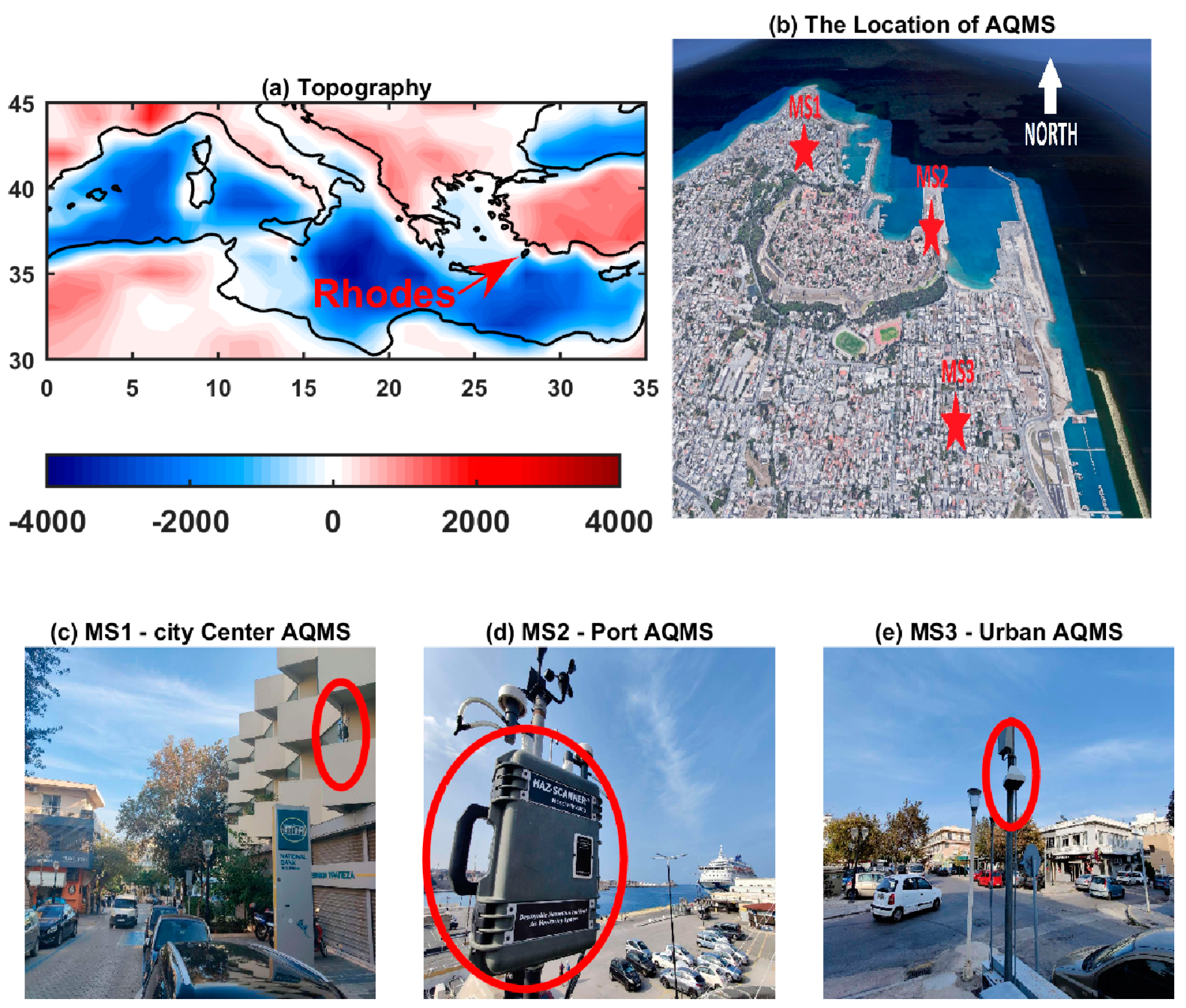
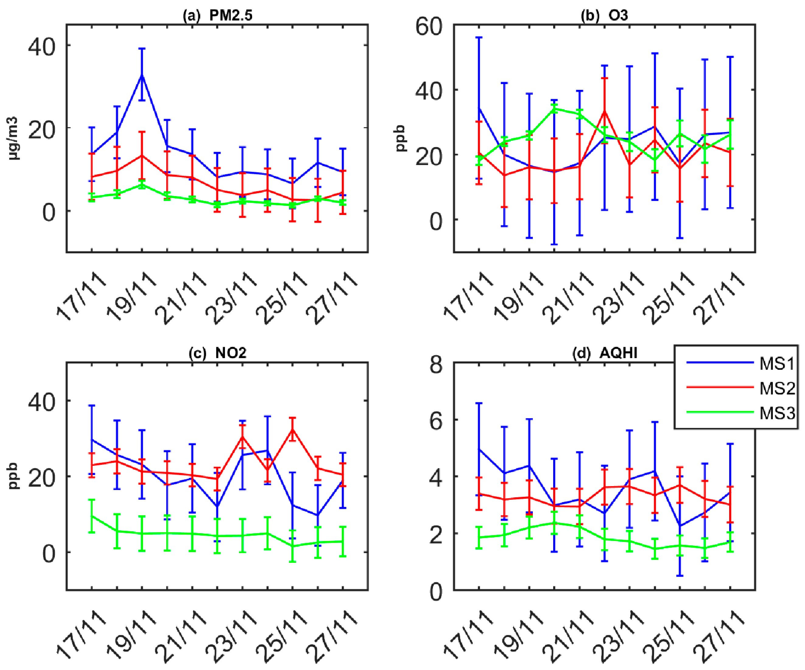
3.1. Comparing Air Quality and AQHI in Three Different Areas in Rhodes City

Figure 2 shows the daily mean variation of pollutants concentration and AQHI for the city center (MS1), port (MS2) and urban (MS3) areas of Rhodes city. The concentration of PM 2.5 is increased in MS1 compared to other regions (Figure 2a). Higher traffic emissions and anthropogenic activities in the city center (MS1) appear to be a significant factor affecting the daily mean concentration levels of PM 2.5 . The traffic emissions and commercial activities are likely the cause of the worsened air quality in MS1 area, compared to MS2 and MS3. Artíñano et al. [83] and Yanosky et al. [30] have shown that PM 2.5 concentration is highly related to the level of traffic emissions. According to the Air Quality Guidelines (AQG) from the WHO in 2021 [11], the maximum PM 2.5 concentrations occurring on 18 and 19 November (about 18 μg/m3 and 39 μg/m3, respectively) exceeded the threshold of the daily mean limit (15 μg/m3). The analysis shows that the concentration of O 3 presents a slight increase in MS3 area when compared to the MS1 and MS2 (Figure 2b). The local chemistry reactions brought on by higher traffic emissions at MS1 and MS2 stations over the timeframe from 19 November to 21 November may account for the lower O 3 concentrations observed there. The higher emissions, due to the increased vehicles exhaust emissions in the city center (MS1) and port (MS2) area, as compared to the urban area (MS3), possibly affect the level of VOCs concentration affecting the level of O 3 concentration [25]. Additionally, the vehicular emissions of NO X is a main precursor for O 3 . Generally, there is a nonlinear relation between O 3 and their precursors (VOCs and NOx) that contribute to the O 3 formation [27,84,85]. Air quality in urban environments is sensitive to meteorological conditions which influence the VOC/ NO X ratio, for instance, through the vertical mixing mechanisms in the boundary layer [85]. Moreover, the meteorological parameters such as wind speed, potentially affect NO X and O 3 variability. The higher level of NO X over the city center, as a result of higher traffic emissions compared to MS2 and MS3, possibly explains the differences among the concentration of O 3 over these areas. Regarding AQHI, the analysis shows that the calculated index values are classified as the Moderate health risk class for the city center of Rhodes (MS1), during 17 to 19, and the 23 and 24 November, 2022. This finding suggests that during these days, the mean population does not need to modify their usual outdoor activities, but the sensitive part of population should be aware of health symptoms such as cough and throat irritation [86,87,88,89]. The AQHI for the port and urban area shows that the health danger is Low and no measures are recommended to be adopted by the population (Figure 2d).
In order to further investigate the different level of pollution among the city center, port, and urban areas, the daily mean anomalies of the concentration of pollutants and AQHI of MS1 and MS2 with reference to MS3 are calculated. In particular, the difference between MS1 and MS3, as well as MS2 and MS3, are calculated (Figure 3). The analysis shows that PM 2.5 in the city center (MS1), compared to the urban area (MS3), is increased from 17 to 21 November (about 10 to 28 μg/m3) and from 26 to 27 November (about 8 μg/m3) (Figure S1a). The daily mean changes of PM 2.5 concentrations over the port (MS2), with reference to the urban station (MS3), show insignificant positive changes (about 5 μg/m3). For the concentration of O 3 , the analysis shows insignificant changes for both MS1 and MS2, relative to MS3 (Figure S1b). The high variability of O 3 , the impact of atmospheric chemistry reactions on O 3 levels, as well as the traffic (vehicle) emissions, determine the concentration of the pollutants’ levels and the variability of O 3 [85]. The NO 2 in the city center (MS1) is increased (about 15 ppb) compared to the urban station (MS3) on the 17 to 19, 23 to 24 and 27 of November 2022. For the MS1 area, NO 2 concentrations show an insignificant increase of about 0 to 10 ppb, except on the 23 and 24 November, when the NO 2 concentration increased to about 20 ppb (Figure S1c). The level of NO 2 differences between MS1 to MS3 and MS2 to MS3 differ by about 15 ppb during the 17 to 24 November. The daily mean AQHI for MS1, compared to MS3, is shown to be increased by about 1.0 to 3.0. For the MS2, the analysis also shows increased values of AQHI (about 0.5 to 2.0; Figure S1d).
In summary, the worst air quality (in terms of PM 2.5 , NO 2 and O 3 ) and the higher health risk for the population (in terms of AQHI) among the studied areas (MS1, MS2 and MS3), are presented over the city center area (MS1). Increased traffic and vehicular emissions, as well as the human activities, seem to determine the level of pollution and the health risk for the population, thus degrading the ambient air quality in the city center area. Traffic exhaust gases have been demonstrated to worsen the quality of the surrounding air throughout previous investigations [6,7,23,24]. Additionally, traffic-related emissions affect people’s health and are associated with health disorders and a variety of diseases [86,87,88,89].
Figure 3 shows the mean diurnal variability of pollutants’ concentration and AQHI during the studied period. The PM 2.5 concentration increases during the hours between 13:00 and 21:00 for the city center (MS1) and port (MS2) areas. During these hours, the mean concentration of PM 2.5 over MS1 is about 18 μg/m3 and over MS2 about 10 μg/m3, respectively (Figure 3a). For MS3 (urban area), the diurnal variation shows an insignificant evolution during the mean day of the studied period (Figure 3a). The lower traffic activity over MS3, compared to MS2 areas (and especially MS1), provides an explanation for the lower concentration of PM 2.5 in MS3, compared to the rest studied areas. The diurnal variation of the concentration of O 3 for the MS1 area shows an increase from morning to evening hours. Generally, the impact of chemical reaction and the diurnal solar radiation affects the concentration of O 3 in the near-surface tropospheric layer. Traffic emissions are a significant source of NO X and VOCs on an urban scale, and are also a fundamental precursor for other pollutants such as O 3 [85,90,91,92,93,94,95,96]. Due to the anthropogenic activities, the VOCs possibly affect the concentration of O 3 during daytime hours [85]. MS1 is located on a high-traffic commercial road in Rhodes city center. Man-made activities, such as vehicle and traffic density, as well as traffic congestion, were maximized during the hours between 14:00 to 16:00. The high-traffic activity during these hours possibly affects the local chemical production of O 3 [94,95,96]. For MS2, the concentration of O 3 peaks at midday. The variation of hourly mean O 3 concentration of MS3 shows a peak during 12:00 to 15:00. The mean diurnal cycle of O 3 over the studied areas shows that the traffic activity over MS3 is lower than the other two areas (MS1 and MS2). This element demonstrates that high traffic affects air quality over the city’s areas. The concentration of NO 2 shows a typical diurnal variability [91,92]. In particular, the analysis shows a reduction during the hours between 12:00 and 15:00 for the MS1 (city center) and MS2 (port). The diurnal cycle of NO 2 concentration for MS3 does not show significant variation during the mean day over the studied period (Figure 3c). As previously mentioned, the reduced traffic volume over this region may be to blame for the negligible hourly change in NO 2 concentration. Additionally, the variability for both O 3 and NO 2 is affected by traffic and anthropogenic emissions (such as VOCs, solar cycle), and meteorological factors such as wind speed, temperature, relative humidity, cloud cover, precipitation, etc. [25,26,27,28,48,49,50,51,52,53,92,94,95,96,97,98]. The calculation of the diurnal variation of the AQHI shows that the air quality, most significantly, affects people’s health during the night and evening hours (Figure 3d) for the city center (MS1) area. The main reason for this point is that, during these hours, the concentration of the studied pollutants was maximized or maintained at a high level compared to other hours during the mean day of the period under study. For MS2, the diurnal variation of the AQHI shows that daytime hours present AQHI values classified in the (limited) Moderate class (about 3.0 to 4.0). Results show that the variation of pollutant concentrations affect people’s health risk.
To further investigate the differences in air quality and AQHI among city center (MS1), port (MS2) and urban areas (MS3), the diurnal anomalies for the concentration of pollutants and AQHI over the MS1 to MS3 (MS1–MS3) and MS2 to MS3 (MS2–MS3), are shown in Figure S2. The analysis shows that the hourly anomalies of the concentration of PM 2.5 over the MS1 area are increased by about 10 to 15 μg/m3, compared to the MS3 area. The MS2 area shows insignificant positive diurnal anomalies compared to MS3 (about 5 to 9 μg/m3; Figure S2a). Regarding the diurnal anomalies of the O 3 concentration, the analysis generally indicates insignificant changes. An exception is MS2, where negative significant differences of about −5 to −11 ppb are shown during 3:00 to 9:00 (Figure S2b). The diurnal anomalies of NO 2 , both for MS1 and MS2 (as compared to MS3), are generally (significant) positive (Figure S2c). The MS1 shows a reduction of the NO 2 concentration during daytime hours following a standard variation of NO 2 . In general, NO 2 variability is associated with the traffic emissions and also the diurnal variation due to chemical reactions between O 3 and NO X [92,94]. The diurnal variation of AQHI shows positive anomalies of about 1.0 to 3.0, as a result of the diurnal variation of concentration of PM 2.5 , O 3 and NO 2 (Figure S2d). This finding indicates that health risks are, in general, increased over the high-traffic congestion hours in the city center (MS1) and port areas (MS2), in comparison to the urban area (MS3). The analyses of Wang et al. [93] and Huang et al. [97] provide elements that vehicle emissions are an important source of pollutants increasing the health risks of the population. Additionally, emissions during peak vehicle traffic hours have a substantial impact on human health [98]. The report by the European Environment Agency [99] stated that a significant proportion of NO X and PM 2.5 concentration comes from traffic activities causing disturbances to human health. Finally, the analysis by Chen et al. [100] has shown that traffic pollution is associated with important health disorders regarding COVID-19 infections. These data indicate the impact of air quality degradation on human health, and are in line with the results of this analysis (the increased values of AQHI over the high-traffic activity hours).

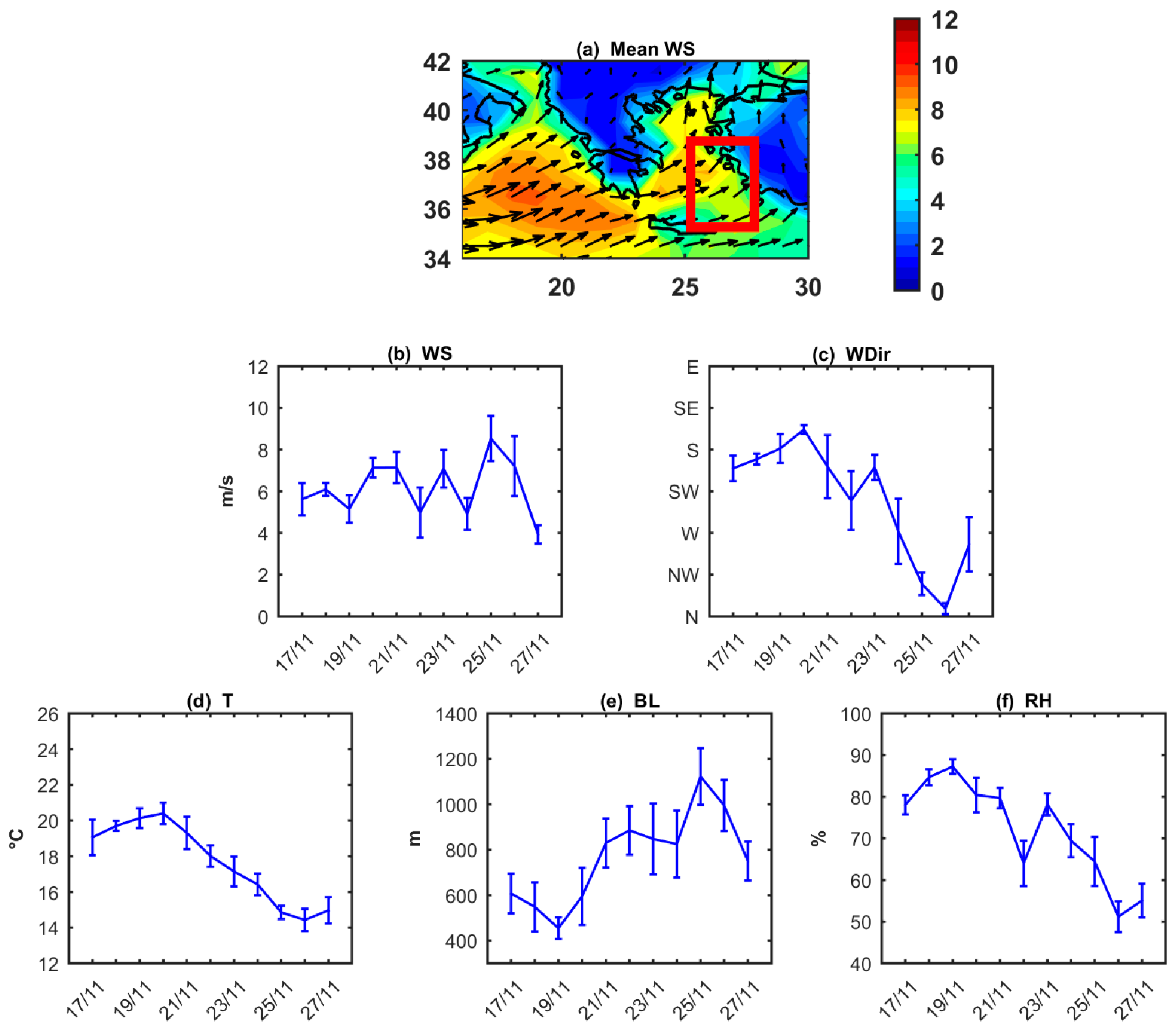
3.2. The Impact of Meteorology and Atmospheric Circulation on the Air Quality and AQHI in Rhodes City

As already mentioned, meteorological factors significantly affect the variability and the level of pollutants over an area. In order to investigate the impact of meteorological factors on the variation of pollutants and AQHI, hourly values of the meteorological variables from ERA5 reanalysis are analyzed. Figure 4a shows the composite mean of the wind speed and direction over an extended region, which includes the Aegean Sea and Rhodes Island. The analysis indicates that the dominant wind directions during the studied period blow from the south–southwest to north–northwest sectors (SSW–W–NNW). In order to investigate the impact of wind speed and direction on the pollutants concentration level and AQHI, hourly wind speed/direction, as well as temperature at 2 m, boundary layer height, and relative humidity, are calculated over a domain of the southeastern Aegean Sea (seAeg) near Rhodes Island (from 25° to 28° E and 35° to 39° N). Figure 4b–f indicates the daily mean variation of wind speed (WS; m/s), wind direction (WDir; °) temperature at 2 m (T; °C), height of boundary layer (BL; m) and relative humidity (RH, %) averaged over the seAeg.
In order to study the relation between the level of pollution (concentration of pollutants, as well as AQHI), in Rhodes city, and the meteorological conditions over the region of Rhodes Island, the Pearson correlation coefficients among the hourly concentration of pollutants (as well as AQHI) and meteorological factors averaged over the seAeg region, are calculated. The results of this analysis are shown in Table 2. Generally, the wind speed shows a negatively low correlation with the majority of the pollutants concentration in the MS1, MS2 and MS3 areas (statistically significant correlation values for MS1 and MS2 areas). Wind direction and the concentration of PM 2.5 show positive correlation for studied areas (about 0.34). Over the MS3 region, the wind direction is positively related to the concentration of NO 2 and AQHI. The higher correlation values between wind direction and pollutants in MS3 region, compared to other areas, are possibly explained by the traffic emissions and the building plan of the regions. Temperature at 2 m (T) is positively related to the concentration of PM 2.5 for each area and also to the concentration of all studied pollutants in MS3 area. It is possibly explained by the common hourly variation of traffic activity and temperature in the city during daytime hours. Mendes et al. [101] have shown that wind speed (WS) and temperature (T) is associated with the concentration of O 3 , but the O 3 episodes are significantly related to the ratio of VOCs/ NO X . Previous studies have shown that the increase in temperature usually tends to reduce the PMs, but there are many other factors and mechanisms that may change this relation in urban environments [102,103]. The analysis indicates that the height of boundary layer (BL) shows negative (moderate) correlation values to the concentration of PM 2.5 and NO 2 (except the concentration of NO 2 over MS2 area). The relative humidity (RH) shows positive correlation values to the concentration of PM 2.5 in studied areas. Generally, the increased humidity make the PMs moister and reduce their dispersion, affecting the rise of the concentration of PM2.5 [104]. Finally, for the MS1 and MS3 areas, the correlation between relative humidity and the concentration of NO 2 , as well as AQHI, is positive.
In order to further investigate the possible association between wind speed and the level of pollution, the OR can be calculated. In the analysis, the outcome is the low (high) concentration of pollutants and AQHI. The exposure is the intense (weak) wind speed. Table 3 shows the OR, CI (Confidence Intervals) at 95%, and the p-values for each of the pollutants of AQMS. For the MS1 (city center), the OR for all pollutants and AHQI are higher from the null value (one) and also statistically significant. This result indicates that there is a statistically significant relation between the intense wind speed and low concentration of pollutants over the city center of Rhodes. For the MS2 (port), the intense wind speed seems to be associated with the low concentration for PM 2.5 and O 3 , as well as with AQHI. However, the intense wind speed is statistically significantly related only with the low concentration of PM 2.5 . In other cases, the CI includes the null value. Finally, for the MS3 (urban area), the intense wind speed is related to the low concentration of PM 2.5 and NO 2 (OR > 1 but statistically insignificant at 95%). These findings show that the wind speed affects the pollution level and AQHI for Rhodes city (mainly for the city center of Rhodes) during the studied period (from 17 to 27 November 2022). Results over this period indicate that wind speed tends to reduce the pollutants concentrations but is not statistically significant in all cases.
Following the methodology of the previous paragraph, the OR is calculated in order to study the association between wind direction and pollution level. Here, the outcome is the low (high) concentration of pollutants and AQHI. The exposure is the north (south) sector wind direction. Results of this analysis are shown in Table 4. For the MS1 (city center), the south sector winds are associated with the higher concentration of PM 2.5 and NO 2 . The health risk for people also worsens as a result of the (statistically significant) greater than null value (one) OR for the concentration of PM 2.5 and NO 2 . For the MS2 (port), the south wind directions seem to be associated with the increased concentration of PM 2.5 (statistically significant) and O 3 (statistically insignificant). For the MS3 (urban area), the south wind direction is associated with the increased concentration of pollutants and AQHI. Findings indicate that the recordings of all AQMS show that the south sector winds are associated with the increased concentration of PM 2.5 . In order to investigate this point further, we studied dust concentration images, which were provided by the WMO Barcelona Dust Regional Center and the partners of the SDS-WAS for Northern Africa, the Middle East and Europe. The images show that a dust transfer episode from 18 to 21 November possibly affects the region of Rhodes Island (Figure S3). Furthermore, this episode is quite possibly the cause of a large transport of particulate matter from Africa to southeastern Mediterranean, affecting the level of PM 2.5 in the city of Rhodes. Additionally, during the episode days, the average height of the boundary layer (BL) was lower by about 250 m, compared to the non-episode days. The combination of the traffic emissions, atmospheric circulation features (dust episode), and the reduction in the height of boundary layer between dust episode and non-dust episode days, possibly explains the changes in the level of PM 2.5 concentration. In particular, on the days of the episode, compared to the other days (17 and from 22 to 27 November 2022), the concentration of PM 2.5 is increased by about 10.5 μg/m3 for MS1, 5.4 μg/m3 for MS2, and 2.0 μg/m3 for MS3. In other words, during these days the AQMS show an increase of PM 2.5 concentration of about 48–54%, compared to the other, non-episode days. Generally, the atmospheric dynamics of tropical and subtropical regions affect the atmospheric circulation over the eastern Mediterranean [43,54,55,58,59]. The air quality and the level of particulate matter over the Greek domain is prone to atmospheric circulation patterns, such as African transfer episodes [40,59]. The results of our analysis possibly indicate that the African dust episode affects the level of pollution over Rhodes city, providing an additive contribution (except for the traffic emissions) to the degradation of the air quality. The most significant degradation of air occurs in the city center of Rhodes.

4. Conclusions

This work examines the variation in air quality conditions and the resulting health impacts on the local population in three different locations over the city of Rhodes, located in the southeastern Mediterranean. The measurement study covers the period from 17 to 27 November 2022. This study tries to shed light on the air quality and the possible impact of wind patterns on the level of pollution during a low-traffic density period for Rhodes city, providing elements among different locations over the city. For the analysis, hourly recordings of PM 2.5 , NO 2 and O 3 concentrations over a city center area, a port and an urban area, using three calibrated mobile Air Quality Monitoring Systems (AQMS), are analyzed. Additionally, the Air Quality Health Index (AQHI) is calculated in order to investigate the effects of pollution levels on the population, over the different areas in the city. Moreover, the possible impact of meteorological factors, such as wind pattern (Wind speed and direction), temperature at 2 m, boundary layer height and relative humidity, as well as the large scale atmospheric circulation on the pollution level and AQHI in the city, are investigated using data from ERA5 reanalysis.
Based on the analysis, the results and the main findings are concluded in the following points:
  • The air quality is more degraded in the city center (MS1) area, compared to port (MS2) and urban (MS3) areas. The concentration of PM 2.5 ( NO 2 ) in the MS1 area is increased by about 78% (76%) with reference to the concentration of PM 2.5 ( NO 2 ) in MS3. The common analysis for the MS2 shows that the concentration of PM 2.5 ( NO 2 ) is increased by about 55% (80%) compared to MS3. These points highlight the importance of vehicle traffic and anthropogenic activities for the air quality in Rhodes city.
  • The highest health risk (in terms of Air Quality Health Index; AQHI) is shown over the city center (MS1) area. The calculation of the daily mean values of AQHI are classified via Low to Moderate health risk classes. AQHI, over MS2 and MS3, shows lower health risks (improved conditions) compared to MS1. The pollution level in MS1, compared to MS3, causes higher AQHI values ranging from 1.0 to 3.0 (a relative increase by about 48%) and the MS2, compared to MS3 which shows higher AQHI values varying from 0.5 to 2.0 (a relative increase by about 43%), respectively.
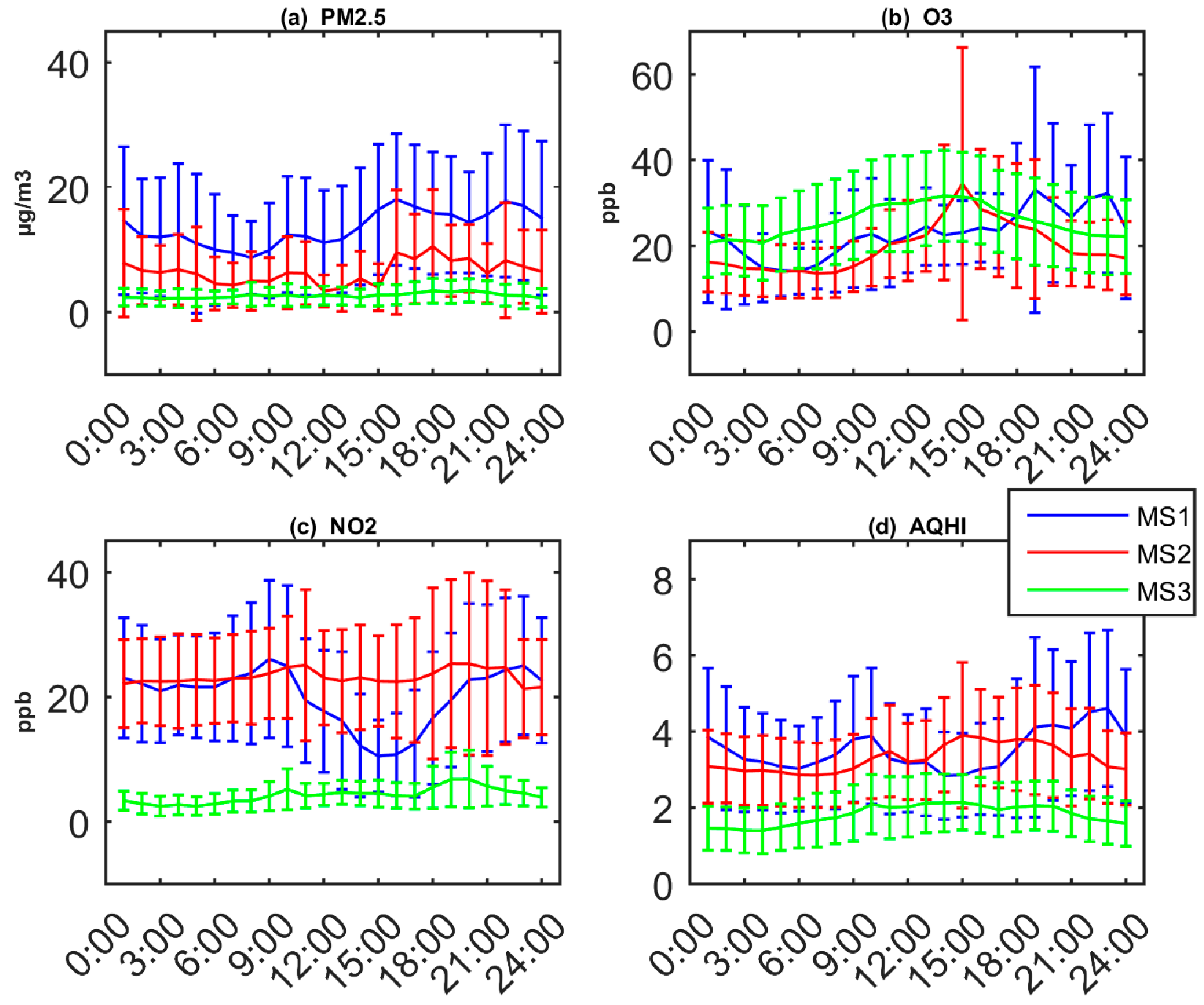
  • The hourly variability of traffic and anthropogenic activities seem to affect the diurnal variation of pollutants. The concentration of PM 2.5 increases during the day (from morning to late evening hours). NO 2   and O 3 appear to follow a typical hourly variation due to atmospheric chemistry and local emissions.
  • The meteorological conditions over the southeastern Aegean seem to affect the variation and level of pollution in Rhodes city. The wind pattern over southeastern Aegean affects the variation and level of pollution. Wind speed tends to reduce the pollutants concentrations (not statistically significant in all cases). Additionally, wind direction seems to affect the concentration of pollutants. South sector winds are associated with the increased concentration of PM 2.5 over the studied areas. Possibly, the large atmospheric circulation contributes to the level of PM 2.5 in the city of Rhodes via the transfer of African dust during a dust episode that affects the southeastern Aegean Sea. The episode occurred during the period from 18 to 21 November, 2022. Moreover, the height of the boundary layer seems to affect the air quality in the city. Results show that the increase of the boundary layer is related to the reduced concentration of pollutants. The temperature and relative humidity show moderate (positive) correlation with PM 2.5 concentrations in all studied areas (MS1, MS2 and MS3). Finally, the analysis indicates that the air quality in the city of Rhodes is affected by vehicle traffic, anthropogenic activities and meteorological conditions.
To sum up, despite the limitations stated, the analysis conducted shows precise elements that highlight the significance of conducting air pollutant measurements, in order to have a better foundation on potential actions that need to be taken to ensure the sustainability of each coastal region. Undeniably, a pilot, such as the examined, or even better, a wider AQMS network, could be considered an economically feasible and viable solution for conducting air pollution studies in highly visited regions where there are no previous air quality recordings, and further research into these areas is essential from a social, economic, and environmental perspective.

Supplementary Materials

The following supporting information can be downloaded at: https://www.mdpi.com/article/10.3390/air1020011/s1, Figure S1. Daily anomalies of (a) PM 2.5 , (b) O 3 , (c) NO 2 concentrations and (d) AQHI between MS1 (city center station) and MS3 (urban station) as well as MS2 (port station) and MS3 (urban station), respectively. Red/blue points show the statistically significant/insignificant differences at 95%. Figure S2. Diurnal anomalies of (a) PM 2.5 , (b) O 3 , (c) NO 2 concentrations and (d) AQHI between MS1 (city center station) and MS3 (urban station) as well as MS1 (city center station) and MS2 (port station), respectively. Red/blue point show the statistically significant/insignificant differences at 95%. Figure S3: Images at 00:00 of the multi-model mean dust surface concentration (μg/m3) during the period from 17 to 27 November 2022. Images were provided by the WMO Barcelona Dust Regional Center. (Source: https://dust.aemet.es/products/daily-dust-products, assessed date: 9 March 2022).

Author Contributions

Conceptualization, I.L., A.M. and P.G.; methodology, I.L.; software, I.L.; validation, I.L.; formal analysis, I.L.; investigation, I.L. and C.A.; resources, I.L.; data curation, I.L. and G.Z.; writing—original draft preparation, I.L.; writing—review and editing, I.L., C.A. and G.Z.; visualization, I.L.; supervision, A.M. and P.G.; project administration, A.M. and P.G.; funding acquisition, P.G. All authors have read and agreed to the published version of the manuscript.

Funding

This research was funded by the Operational Programme “Competitiveness, Entrepreneurship and Innovation” (NSRF 2014–2020) and co-financed by Greece and the European Union (European Regional Development Fund).

Institutional Review Board Statement

Not applicable.

Informed Consent Statement

Not applicable.

Data Availability Statement

Copernicus Climate Change Service (C3S) (2017): ERA5: Fifth generation of ECMWF atmospheric reanalysis of the global climate. Copernicus Climate Change Service Climate Data Store (CDS), date of access. https://cds.climate.copernicus.eu/cdsapp#!/home (assessed on 17 February 2023). Dust data and/or images were provided by the WMO Barcelona Dust Regional Center and the partners of the Sand and Dust Storm Warning Advisory and Assessment System (SDS-WAS) for Northern Africa, the Middle East and Europe. https://dust.aemet.es/products/daily-dust-products (assessed on 8 March 2023).

Acknowledgments

We acknowledge the support of this work by the project “ELEKTRON” (MIS: 5047136), which is implemented under the Action “Reinforcement of the Research and Innovation Infrastructure”, funded by the Operational Programme “Competitiveness, Entrepreneurship and Innovation” (NSRF 2014–2020) and co-financed by Greece and the European Union (European Regional Development Fund). The authors would like to acknowledge Copernicus Climate Change Service that provided the ERA5 climate reanalysis data that were used in this work. Additionally, we would like to acknowledge Dust data and/or images were provided by the WMO Barcelona Dust Regional Center and the partners of the Sand and Dust Storm Warning Advisory and Assessment System (SDS-WAS) for Northern Africa, the Middle East and Europe. Many thanks are given to the Google Earth for providing the imagery that was used in this work. The authors gratefully acknowledge Dimitra Karalli and Konstantinos Rizos for their scientific support and fruitful discussion about the analysis and scientific results. Finally, the authors would like to thank Ourania Hassiltzoglou for English Language editing.

Conflicts of Interest

The authors declare no conflict of interest.

References

  1. Landrigan, P.J.; Fuller, R. Global health and environmental pollution. Int. J. Public Health 2015, 60, 761–762. [Google Scholar] [CrossRef] [PubMed] [Green Version]
  2. Abas, A.; Asnawi, N.H.; Aiyub, K.; Awang, A.; Abdullah, S.R. Lichen Biodiversity Index (LBI) for the Assessment of Air Quality in an Industrial City in Pahang, Malaysia. Atmosphere 2022, 13, 1905. [Google Scholar] [CrossRef]
  3. Nastos, P.T. Weather, Ambient Air Pollution and Bronchial Asthma in Athens, Greece. In Seasonal Forecasts, Climatic Change and Human Health; Thomson, M.C., GarciaHerrera, R., Beniston, M., Eds.; Advances in Global Change Research; Springer: Dordrecht, The Netherlands, 2008; Volume 30. [Google Scholar] [CrossRef]
  4. Monforte, P.; Ragusa, M.A. Evaluation of the air pollution in a Mediterranean region by the air quality index. Environ. Monit. Assess. 2018, 190, 625. [Google Scholar] [CrossRef] [PubMed]
  5. Lovett, G.M.; Tear, T.H.; Evers, D.C.; Findlay, S.E.G.; Cosby, B.J.; Dunscomb, J.K.; Driscoll, C.T.; Weathers, K.C. Effects of Air Pollution on Ecosystems and Biological Diversity in the Eastern United States. Ann. N. Y. Acad. Sci. 2009, 1162, 99–135. [Google Scholar] [CrossRef] [PubMed]
  6. Etim, E.U. Air pollution emission inventory along a major traffic route within Ibadan Metropolis, southwestern Nigeria. Afr. J. Environ. Sci. Technol. 2016, 10, 432–438. [Google Scholar] [CrossRef] [Green Version]
  7. von Schneidemesser, E.; Steinmar, K.; Weatherhead, E.C.; Bonn, B.; Gerwig, H.; Quedenau, J. Air pollution at human scales in an urban environment: Impact of local environment and vehicles on particle number concentrations. Sci. Total Environ. 2019, 688, 691–700. [Google Scholar] [CrossRef]
  8. Narayana, M.V.; Jalihal, D.; Nagendra, S.M.S. Establishing A Sustainable Low-Cost Air Quality Monitoring Setup: A Survey of the State-of-the-Art. Sensors 2022, 22, 394. [Google Scholar] [CrossRef]
  9. Ghosh, R.; Lurmann, F.; Perez, L.; Penfold, B.; Brandt, S.; Wilson, J.; Milet, M.; Künzli, N.; McConnell, R. Near-roadway air pollution and coronary heart disease: Burden of disease and potential impact of a greenhouse gas reduction strategy in southern California. Environ. Health Perspect. 2016, 124, 193–200. [Google Scholar] [CrossRef] [Green Version]
  10. Hegseth, M.N.; Oftedal, B.M.; Höper, A.C.; Aminoff, A.L.; Thomassen, M.R.; Svendsen, M.V.; Fell, A.K.M. Self-reported traffic-related air pollution and respiratory symptoms among adults in an area with modest levels of traffic. PLoS ONE 2019, 14, e0226221. [Google Scholar] [CrossRef] [Green Version]
  11. World Health Organization. WHO Global Air Quality Guidelines: Particulate Matter (PM2.5 and PM10), Ozone, Nitrogen Dioxide, Sulfur Dioxide and Carbon Monoxide. World Health Organization. 2021. Available online: https://apps.who.int/iris/handle/10665/345329 (accessed on 23 March 2023).
  12. World Health Organization. Regional Office for Europe & Joint WHO/Convention Task Force on the Health Aspects of Air Pollution. In Health Risks of Particulate Matter from Long-Range Transboundary Air Pollution; WHO Regional Office for Europe: Copenhagen, Denmark, 2006. Available online: https://apps.who.int/iris/handle/10665/107691 (accessed on 23 March 2023).
  13. IPCC. Special Report Global Warming of 1.5 °C. Available online: https://www.ipcc.ch/sr15/ (accessed on 10 March 2023).
  14. IPCC. Climate Change 2022: Impacts, Adaptation, and Vulnerability. Contribution of Working Group II to the Sixth Assessment Report of the Intergovernmental Panel on Climate Change; Pörtner, H.-O., Roberts, D.C., Tignor, M., Poloczanska, E.S., Mintenbeck, K., Alegría, A., Craig, M., Langsdorf, S., Löschke, S., Möller, V., et al., Eds.; Cambridge University Press: Cambridge, UK; New York, NY, USA, 2022; 3056p. [Google Scholar] [CrossRef]
  15. Sarmadi, M.; Rahimi, S.; Rezaei, M.; Sanaei, D.; Dianatinasab, M. Air quality index variation before and after the onset of COVID-19 pandemic: A comprehensive study on 87 capital, industrial and polluted cities of the world. Environ. Sci. Eur. 2021, 33, 134. [Google Scholar] [CrossRef]
  16. Chakraborty, P.; Jayachandran, S.; Padalkar, P.; Sitlhou, L.; Chakraborty, S.; Kar, R.; Bhaumik, S.; Srivastava, M. Exposure to nitrogen dioxide (NO2) from vehicular emission could increase the COVID-19 pandemic fatality in India: A perspective. Bull. Environ. Contam. Toxicol. 2020, 105, 198–204. [Google Scholar] [CrossRef] [PubMed]
  17. Yamamoto, S.S.; Phalkey, R.; Malik, A.A. A systematic review of air pollution as a risk factor for cardiovascular disease in South Asia: Limited evidence from India and Pakistan. Int. J. Hyg. Environ. Health 2014, 217, 133–144. [Google Scholar] [CrossRef] [PubMed]
  18. Rumana, H.S.; Sharma, R.C.; Beniwal, V.; Sharma, A.K. A retrospective approach to assess human health risks associated with growing air pollution in urbanized area of Thar Desert, Western Rajasthan, India. J. Environ. Health Sci. Eng. 2014, 12, 23. [Google Scholar] [CrossRef] [PubMed] [Green Version]
  19. Orellano, P.; Quaranta, N.; Reynoso, J.; Balbi, B.; Vasquez, J. Effect of outdoor air pollution on asthma exacerbations in children and adults: Systematic review and multilevel meta-analysis. PLoS ONE 2017, 12, e0174050. [Google Scholar] [CrossRef] [PubMed]
  20. Vermaelen, K.; Brusselle, G. Exposing a deadly alliance: Novel insights into the biological links between COPD and lung cancer. Pulm. Pharmacol. Ther. 2013, 26, 544–554. [Google Scholar] [CrossRef]
  21. Kan, H.; Chen, B.; Zhao, N.; London, S.J.; Song, G.; Chen, G.; Zhang, Y.; Jiang, L.; HEI Health Review Committee. Part 1. A time-series study of ambient air pollution and daily mortality in Shanghai, China. Res. Rep. Health Eff. Inst. 2010, 154, 17–78. [Google Scholar]
  22. Kuula, J.; Timonen, H.; Niemi, J.V.; Manninen, H.E.; Rönkkö, T.; Hussein, T.; Fung, P.L.; Tarkoma, S.; Laakso, M.; Saukko, E.; et al. Opinion: Insights into updating Ambient Air Quality Directive 2008/50/EC. Atmos. Chem. Phys. 2022, 22, 4801–4808. [Google Scholar] [CrossRef]
  23. Juginović, A.; Vuković, M.; Aranza, I.; Biloš, V. Health impacts of air pollution exposure from 1990 to 2019 in 43 European countries. Sci. Rep. 2021, 11, 22516. [Google Scholar] [CrossRef]
  24. Reche, C.; Tobias, A.; Viana, M. Vehicular Traffic in Urban Areas: Health Burden and Influence of Sustainable Urban Planning and Mobility. Atmosphere 2022, 13, 598. [Google Scholar] [CrossRef]
  25. Deng, Y.; Li, J.; Li, Y.; Wu, R.; Xie, S. Characteristics of volatile organic compounds, NO2, and effects on ozone formation at a site with high ozone level in Chengdu. J. Environ. Sci. 2019, 75, 334–345. [Google Scholar] [CrossRef]
  26. Li, J.; Zhai, C.; Yu, J.; Liu, R.; Li, Y.; Zeng, L.; Xie, S. Spatiotemporal variations of ambient volatile organic compounds and their sources in Chongqing, a mountainous megacity in China. Sci. Total Environ. 2018, 627, 1442–1452. [Google Scholar] [CrossRef] [PubMed]
  27. Liu, T.; Sun, J.; Liu, B.; Li, M.; Deng, Y.; Jing, W.; Yang, J. Factors Influencing O3 Concentration in Traffic and Urban Environments: A Case Study of Guangzhou City. Int. J. Environ. Res. Public Health 2022, 19, 12961. [Google Scholar] [CrossRef] [PubMed]
  28. Mazzuca, G.M.; Ren, X.; Loughner, C.P.; Estes, M.; Crawford, J.H.; Pickering, K.E.; Weinheimer, A.J.; Dickerson, R.R. Ozone production and its sensitivity to NOx and VOCs: Results from the DISCOVER-AQ field experiment, Houston 2013. Atmos. Chem. Phys. Discuss. 2016, 16, 14463–14474. [Google Scholar] [CrossRef] [Green Version]
  29. Mukherjee, A.; McCarthy, M.C.; Brown, S.G.; Huang, S.; Landsberg, K.; Eisinger, D.S. Influence of roadway emissions on near-road PM2.5: Monitoring data analysis and implications. Transp. Res. Part D Transp. Environ. 2020, 86, 102442. [Google Scholar] [CrossRef]
  30. Yanosky, J.D.; Fisher, J.; Liao, D.; Rim, D.; Wal, R.V.; Groves, W.; Puett, R.C. Application and validation of a line-source dispersion model to estimate small scale traffic-related particulate matter concentrations across the conterminous US. Air Qual. Atmos. Health 2018, 11, 741–754. [Google Scholar] [CrossRef]
  31. Doumbia, M.; Toure, N.E.; Silue, S.; Yoboue, V.; Diedhiou, A.; Hauhouot, C. Emissions from the Road Traffic of West African Cities: Assessment of Vehicle Fleet and Fuel Consumption. Energies 2018, 11, 2300. [Google Scholar] [CrossRef] [Green Version]
  32. McCarron, A.; Semple, S.; Braban, C.F.; Swanson, V.; Gillespie, C.; Price, H.D. Public engagement with air quality data: Using health behaviour change theory to support exposure-minimising behaviours. J. Expo. Sci. Environ. Epidemiol. 2022, 33, 321–331. [Google Scholar] [CrossRef] [PubMed]
  33. Cairncross, E.K.; John, J.; Zunckel, M. A novel air pollution index based on the relative risk of daily mortality associated with short-term exposure to common air pollutants. Atmos. Environ. 2007, 41, 8442–8454. [Google Scholar] [CrossRef]
  34. Ghorani-Azam, A.; Riahi-Zanjani, B.; Balali-Mood, M. Effects of air pollution on human health and practical measures for prevention in Iran. J. Res. Med. Sci. 2016, 21, 65. [Google Scholar] [CrossRef]
  35. Spyropoulos, G.C.; Nastos, P.T.; Moustris, K.P. Performance of Aether Low-Cost Sensor Device for Air Pollution Measurements in Urban Environments. Accuracy Evaluation Applying the Air Quality Index (AQI). Atmosphere 2021, 12, 1246. [Google Scholar] [CrossRef]
  36. Olstrup, H. An Air Quality Health Index (AQHI) with Different Health Outcomes Based on the Air Pollution Concentrations in Stockholm during the Period of 2015–2017. Atmosphere 2020, 11, 192. [Google Scholar] [CrossRef] [Green Version]
  37. Chen, L.; Villeneuve, P.J.; Rowe, B.H.; Liu, L.; Stieb, D.M. The Air Quality Health Index as a predictor of emergency department visits for ischemic stroke in Edmonton, Canada. J. Expos. Sci. Environ. Epidemiol. 2014, 24, 358–364. [Google Scholar] [CrossRef] [PubMed]
  38. Szyszkowicz, M.A.; Kousha, T. Emergency department visits for asthma in relation to the Air Quality Health Index: A case-crossover study in Windsor, Canada. Can. J. Public Health 2014, 105, 336–341. [Google Scholar] [CrossRef] [PubMed] [Green Version]
  39. Yao, J.; Stieb, D.M.; Taylor, E.; Henderson, S.B. Assessment of the Air Quality Health Index (AQHI) and four alternate AQHI-Plus amendments for wildfire seasons in British Columbia. Can. J. Public Health 2020, 111, 96–106. [Google Scholar] [CrossRef] [PubMed]
  40. Logothetis, I.; Antonopoulou, C.; Sfetsioris, K.; Mitsotakis, A.; Grammelis, P. A Comparative Case Analysis of Meteorological and Air Pollution Parameters between a High and Low Port Activity Period in Igoumenitsa Port. Eng. Proc. 2021, 11, 33. [Google Scholar] [CrossRef]
  41. Logothetis, I.; Antonopoulou, C.; Sfetsioris, K.; Mitsotakis, A.; Grammelis, P. Comparison Analysis of the Effect of High and Low Port Activity Seasons on Air Quality in the Port of Heraklion. Environ. Sci. Proc. 2021, 8, 3. [Google Scholar]
  42. Shukla, J.; Misra, A.; Sundar, S.; Naresh, R. Effect of rain on removal of a gaseous pollutant and two different particulate matters from the atmosphere of a city. Math. Comput. Model. 2008, 48, 832–844. [Google Scholar] [CrossRef]
  43. Rizos, Κ.; Logothetis, Ι.; Koukouli, Μ.Ε.; Meleti, C.; Melas, D. The influence of the summer tropospheric circulation on the observed ozone mixing ratios at a coastal site in the Eastern Mediterranean. Atmos. Pollut. Res. 2022, 13, 101381. [Google Scholar] [CrossRef]
  44. Cichowicz, R.; Wielgosiński, G.; Fetter, W. Effect of wind speed on the level of particulate matter PM10 concentration in atmospheric air during winter season in vicinity of large combustion plant. J. Atmos. Chem. 2020, 77, 35–48. [Google Scholar] [CrossRef]
  45. Pateraki, S.; Asimakopoulos, D.N.; Flocas, H.A.; Maggos, T.; Vasilakos, C. The role of meteorology on different sized aerosol fractions (PM10, PM2.5, PM2.5–10). Sci. Total Environ. 2012, 419, 124–135. [Google Scholar] [CrossRef]
  46. Aldrin, M.; Haff, I.H. Generalised additive modelling of air pollution, traffic volume and meteorology. Atmos. Environ. 2005, 39, 2145–2155. [Google Scholar] [CrossRef]
  47. Chaloulakou, A.; Kassomenos, P.; Spyrellis, N.; Demokritou, P.; Koutrakis, P. Measurements of PM10 and PM2.5 particle concentrations in Athens, Greece. Atmos. Environ. 2003, 37, 649–660. [Google Scholar] [CrossRef]
  48. Su, T.; Li, Z.; Kahn, R. Relationships between the planetary boundary layer height and surface pollutants derived from lidar observations over China: Regional pattern and influencing factors. Atmos. Chem. Phys. 2018, 18, 15921–15935. [Google Scholar] [CrossRef] [Green Version]
  49. Emeis, S.; Schäfer, K. Remote sensing methods to investigate boundary-layer structures relevant to air pollution in cities. Bound.-Lay. Meteorol. 2006, 121, 377–385. [Google Scholar] [CrossRef]
  50. Liu, Y.; Zhou, Y.; Lu, J. Exploring the relationship between air pollution and meteorological conditions in China under environmental governance. Sci. Rep. 2020, 10, 14518. [Google Scholar] [CrossRef]
  51. Megaritis, A.G.; Fountoukis, C.; Charalampidis, P.E.; Denier van der Gon, H.A.C.; Pilinis, C.; Pandis, S.N. Linking climate and air quality over Europe: Effects of meteorology on PM2.5 concentrations. Atmos. Chem. Phys. 2014, 14, 10283–10298. [Google Scholar] [CrossRef] [Green Version]
  52. Cheng, B.; Ma, Y.; Feng, F.; Zhang, Y.; Shen, J.; Wang, H.; Guo, Y.; Cheng, Y. Influence of weather and air pollution on concentration change of PM2.5 using a generalized additive model and gradient boosting machine. Atmos. Environ. 2021, 255, 118437. [Google Scholar] [CrossRef]
  53. Zhang, L.; Cheng, Y.; Zhang, Y.; He, Y.; Gu, Z.; Yu, C. Impact of Air Humidity Fluctuation on the Rise of PM Mass Concentration Based on the High-Resolution Monitoring Data. Aerosol Air Qual. Res. 2017, 17, 543–552. [Google Scholar] [CrossRef] [Green Version]
  54. Cherchi, A.; Annamalai, H.; Masina, S.; Navarra, A. South Asian summer monsoon and the eastern Mediterranean climate: Themonsoon—Desert mechanism in CMIP5 simulations. J. Clim. 2014, 27, 6877–6903. [Google Scholar] [CrossRef] [Green Version]
  55. Logothetis, I.; Tourpali, K.; Misios, S.; Zanis, P. Etesians and the summer circulation over East Mediterranean in CoupledModel Intercomparison Project Phase 5 simulations: Connections to the Indian summer monsoon. Int. J. Climatol. 2020, 40, 1118–1131. [Google Scholar] [CrossRef]
  56. Giorgi, F. Climate change hot-spots. Geophys. Res. Lett. 2006, 33, L08707. [Google Scholar] [CrossRef]
  57. Jacobson, M.Z. Review of solutions to global warming, air pollution, and energy security. Energy Environ. Sci. 2009, 2, 148–173. [Google Scholar] [CrossRef]
  58. Tyrlis, E.; Lelieveld, J. Climatology and Dynamics of the Summer Etesian Winds over the Eastern Mediterranean. J. Atmos. Sci. 2013, 70, 3374–3396. [Google Scholar] [CrossRef]
  59. Mitsakou, C.; Kallos, G.; Papantoniou, N.; Spyrou, C.; Solomos, S.; Astitha, M.; Housiadas, C. Saharan dust levels in Greece and received inhalation doses. Atmos. Chem. Phys. 2008, 8, 7181–7192. [Google Scholar] [CrossRef] [Green Version]
  60. Kallos, G.; Astitha, M.; Katsafados, P.; Spyrou, C. Long-range transport of anthropogenically and naturally produced particulate matter in the Mediterranean and North Atlantic: Current state of knowledge. J. Appl. Meteorol. Clim. 2007, 46, 1230–1251. [Google Scholar] [CrossRef] [Green Version]
  61. Logothetis, I.; Antonopoulou, C.; Zisopoulos, G.; Mitsotakis, A.; Grammelis, P. The Impact of Climate Conditions and Traffic Emissions on the Pms Variations in Rhodes City during the Summer of 2021. In Proceedings of the 7th World Congress on Civil, Structural, and Environmental Engineering (CSEE’22), Virtual Conference, 10–12 April 2022. Paper No. ICEPTP 181. [Google Scholar] [CrossRef]
  62. Bai, L.; Huang, L.; Wang, Z.; Ying, Q.; Zheng, J.; Shi, X.; Hu, J. Long-term Field Evaluation of Low-cost Particulate Matter Sensors in Nanjing. Aerosol Air Q. Res. 2020, 20, 242–253. [Google Scholar] [CrossRef]
  63. Samad, A.; Obando Nuñez, D.R.; Solis Castillo, G.C.; Laquai, B.; Vogt, U. Effect of Relative Humidity and Air Temperature on the Results Obtained from Low-Cost Gas Sensors for Ambient Air Quality Measurements. Sensors 2020, 20, 5175. [Google Scholar] [CrossRef] [PubMed]
  64. Giordano, M.R.; Malings, C.; Pandis, S.N.; Presto, A.A.; McNeill, V.F.; Westervelt, D.M.; Beekmann, M.; Subramanian, R. From low-cost sensors to high-quality data: A summary of challenges and best practices for effectively calibrating low-cost particulate matter mass sensors. J. Aerosol Sci. 2021, 158, 105833. [Google Scholar] [CrossRef]
  65. Liang, L. Calibrating low-cost sensors for ambient air monitoring: Techniques, trends, and challenges. Environ. Res. 2021, 197, 111163. [Google Scholar] [CrossRef] [PubMed]
  66. deSouza, P.; Kahn, R.; Stockman, T.; Obermann, W.; Crawford, B.; Wang, A.; Crooks, J.; Li, J.; Kinney, P. Calibrating networks of low-cost air quality sensors. Atmos. Meas. Tech. 2022, 15, 6309–6328. [Google Scholar] [CrossRef]
  67. Williams, R.; Long, R.; Beaver, M.; Kaufman, A.; Zeiger, F.; Heimbinder, M.; Heng, I.; Yap, R.; Acharya, B.; Grinwald, B.; et al. Sensor Evaluation Report; EPA/600/R-14/143 (NTIS PB2015-100611); Office of Research and Development (8101R): Research Triangle Park, NC, USA; Washington, DC, USA, 2014. Available online: https://cfpub.epa.gov/si/si_public_record_report.cfm?Lab=NERL&dirEntryId=277270&simpleSearch=1&searchAll=sensor+evaluation+report (accessed on 15 April 2023).
  68. Achieng’, G.O.; Andala, D.M. Determination of Ambient air quality status through Assessment of particulate matter and selected gases. In Proceedings of the International Conference on Air Quality in Africa (ICAQ’Africa2022), Virtual, 11–14 October 2022. [Google Scholar]
  69. Environmental Devises Corporation. Haz-Scanner™ model HIM-6000. Available online: https://environmentaldevices.com/him-6000-2/ (accessed on 24 May 2023).
  70. Bencs, L.; Plósz, B.; Mmari, A.G.; Szoboszlai, N. Comparative Study on the Use of Some Low-Cost Optical Particulate Sensors for Rapid Assessment of Local Air Quality Changes. Atmosphere 2022, 13, 1218. [Google Scholar] [CrossRef]
  71. Wahlborg, D.; Björling, M.; Mattsson, M. Evaluation of field calibration methods and performance of AQMesh, a low-cost air quality monitor. Environ. Monit. Assess. 2021, 193, 251. [Google Scholar] [CrossRef] [PubMed]
  72. AQMesh Small Sensor Air Quality Monitoring System. Available online: https://www.aqmesh.com/products/aqmesh/ (accessed on 24 May 2023).
  73. Stieb, D.M.; Burnett, R.T.; Smith-Doiron, M.; Brion, O.; Shin, H.H.; Economou, V. A new multipollutant, no-threshold air quality health index based on short-term associations observed in daily time-series analyses. J. Air Waste Manag. Assoc. 2008, 58, 435–450. [Google Scholar] [CrossRef] [PubMed] [Green Version]
  74. Wilks, D.S. Statistical Methods in the Atmospheric Sciences; Academic Press: New York, NY, USA, 1995. [Google Scholar]
  75. Hersbach, H.; Bell, B.; Berrisford, P.; Hirahara, S.; Horányi, A.; Muñoz-Sabater, J.; Nicolas, L.; Peubey, C.; Radu, R.; Schepers, D.; et al. The ERA5 global reanalysis. QJRMeteorol Soc. 2020, 146, 1999–2049. [Google Scholar] [CrossRef]
  76. Magnus, G. Versuche über die Spannkräfte des Wasserdampfs. Ann. Phys. 1844, 137, 225–247. [Google Scholar] [CrossRef] [Green Version]
  77. August, E.F. Ueber die Berechnung der Expansivkraft des Wasserdunstes. Ann. Phys. 1828, 89, 122–137. [Google Scholar] [CrossRef] [Green Version]
  78. Gibbins, C.J. A survey and comparison of relationships for the determination of the saturation vapour pressure over plane surfaces of pure water and of pure ice. Ann. Geophys. 1990, 8, 859–885. [Google Scholar]
  79. Alduchov, O.A.; Eskridge, R.E. Improved Magnus form approximation of saturation vapor pressure. J. Appl. Meteor. 1996, 35, 601–609. [Google Scholar] [CrossRef]
  80. Stephenson, D.B. Use of the “odds ratio” for diagnosing forecast skill. Weather Forecast. 2000, 15, 221–232. [Google Scholar] [CrossRef]
  81. Altman, D.G.; Bland, J.M. How to obtain the confidence interval from a P value. BMJ 2011, 342, d2090. [Google Scholar] [CrossRef] [Green Version]
  82. Basart, S.; Nickovic, S.; Terradellas, E.; Cuevas, E.; García-Pando, C.P.; García-Castrillo, G.; Werner, E.; Benincasa, F. The WMO SDS-WAS Regional Center for Northern Africa, Middle East and Europe. E3S Web Conf. 2019, 99, 04008. [Google Scholar] [CrossRef]
  83. Artíñano, B.; Salvador, P.; Alonso, D.G.; Quero, X.; Alastuey, A. Influence of traffic on the PM10 and PM2.5 urban aerosol fractions in Madrid (Spain). Sci. Total Environ. 2004, 334–335, 111–123. [Google Scholar] [CrossRef] [PubMed]
  84. Ma, W.; Feng, Z.; Zhan, J.; Liu, Y.; Liu, P.; Liu, C.; Ma, Q.; Yang, K.; Wang, Y.; He, H. Influence of photochemical loss of volatile organic compounds on understanding ozone formation mechanism. Atmos. Chem. Phys. 2022, 22, 4841–4851. [Google Scholar] [CrossRef]
  85. Berezina, E.; Moiseenko, K.; Skorokhod, A.; Pankratova, N.V.; Belikov, I.; Belousov, V.; Elansky, N.F. Impact of VOCs and NOx on Ozone Formation in Moscow. Atmosphere 2020, 11, 1262. [Google Scholar] [CrossRef]
  86. Abelsohn, A.; Stieb, D.M. Health effects of outdoor air pollution: Approach to counseling patients using the Air Quality Health Index. Can. Fam. Phys. 2011, 57, 881–887. [Google Scholar]
  87. Gutenberg, S. Demystifying the air quality health index. Can. Pharm. J. 2014, 147, 332–334. [Google Scholar] [CrossRef] [Green Version]
  88. Manisalidis, Ι.; Stavropoulou, Ε.; Stavropoulos, A.; Bezirtzoglou, Ε. Environmental and Health Impacts of Air Pollution: A Review. Front. Public Health 2020, 8, 14. [Google Scholar] [CrossRef] [Green Version]
  89. Drakaki, E.; Dessinioti, C.; Antoniou, C.V. Air pollution and the skin. Front. Environ. Sci. 2014, 2, 11. [Google Scholar] [CrossRef] [Green Version]
  90. An, J.; Shi, Y.; Wang, J.; Zhu, B. Temporal Variations of O3 and NOx in the Urban Background Atmosphere of Nanjing, East China. Arch. Environ. Contam. Toxicol. 2016, 71, 224–234. [Google Scholar] [CrossRef]
  91. Dainius, J.; Vaida, V.; Renata, C.I.; Milda, P.I. Surface ozone concentration and its relationship with UV Radiation, Meteorological Parameters and Radon on the Eastern Coast of the Baltic Sea. Atmosphere 2016, 7, 27. [Google Scholar]
  92. Qin, Y.; Liu, M.; Song, J.; Yu, R.; Li, L.; Su, J. The temporal and spatial variation characteristics of near-surface O3 concentration in Guangdong-Hong Kong-Macao Greater Bay Area. J. Environ. Sci. 2021, 41, 2987–3000. [Google Scholar]
  93. Wang, P.; Zhang, R.; Sun, S.; Gao, M.; Zheng, B.; Zhang, D.; Zhang, Y.; Carmichael, G.R.; Zhang, H. Aggravated air pollution and health burden due to traffic congestion in urban China. Atmos. Chem. Phys. 2023, 23, 2983–2996. [Google Scholar] [CrossRef]
  94. Pancholi, P.; Kumar, A.; Bikundia, D.S.; Chourasiya, S. An observation of seasonal and diurnal behavior of O3–NOx relationships and local/regional oxidant (OX = O3 + NO2) levels at a semi-arid urban site of western India. Sustain. Environ. Res. 2018, 28, 79–89. [Google Scholar] [CrossRef]
  95. Juráň, S.; Šigut, L.; Holub, P.; Fares, S.; Klem, K.; Grace, J.; Urban, O. Ozone flux and ozone deposition in a mountain spruce forest are modulated by sky conditions. Sci. Total Environ. 2019, 672, 296–304. [Google Scholar] [CrossRef] [PubMed]
  96. Dang, R.; Liao, H.; Fu, Y. Quantifying the anthropogenic and meteorological influences on summertime surface ozone in China over 2012–2017. Sci. Total Environ. 2021, 754, 142394. [Google Scholar] [CrossRef] [PubMed]
  97. Huang, Y.; Unger, N.; Harper, K.; Heyes, C. Global climate and human health effects of the gasoline and diesel vehicle fleets. GeoHealth 2020, 4, e2019GH000240. [Google Scholar] [CrossRef] [Green Version]
  98. Requia, W.G.; Higgins, C.D.; Adams, M.D.; Mohamed, M.; Koutrakis, P. The health impacts of weekday traffic: A health risk assessment of PM2.5 emissions during congested periods. Environ. Int. 2018, 111, 164–176. [Google Scholar] [CrossRef]
  99. European Environment Agency. Air Quality in Europe—2019 Report; Publication Office of European Union, European Environment Agency Kongens Nytorv: Copenhagen, Denmark, 2019; 99p, ISBN 978-92-9480-088-6. [CrossRef]
  100. Chen, Z.; Huang, B.Z.; Sidell, M.A.; Chow, T.; Eckel, S.P.; Pavlovic, N.; Martinez, M.P.; Lurmann, F.; Thomas, D.C.; Gilliland, F.D.; et al. Near-roadway air pollution associated with COVID-19 severity and mortality—Multiethnic cohort study in Southern California. Environ. Int. 2021, 157, 106862. [Google Scholar] [CrossRef]
  101. Mendes, D.; Dantas, G.; André da Silva, M.; Guedes de Seixas, E.; Martins da Silva, C.; Arbilla, G. Impact of the Petrochemical Complex on the Air Quality of an Urban Area in the City of Rio de Janeiro, Brazil. Bull. Environ. Contam. Toxicol. 2020, 104, 438–443. [Google Scholar] [CrossRef]
  102. Kirešová, S.; Guzan, M. Determining the Correlation between Particulate Matter PM10 and Meteorological Factors. Eng 2022, 3, 343–363. [Google Scholar] [CrossRef]
  103. Yang, W.; Wang, G.; Bi, C. Analysis of Long-Range Transport Effects on PM2.5 during a Short Severe Haze in Beijing, China. Aerosol Air Qual. Res. 2017, 17, 1610–1622. [Google Scholar] [CrossRef]
  104. Jiang, B.; Sun, C.; Mu, S.; Zhao, Z.; Chen, Y.; Lin, Y.; Qiu, L.; Gao, T. Differences in Airborne Particulate Matter Concentration in Urban Green Spaces with Different Spatial Structures in Xi’an, China. Forests 2022, 13, 14. [Google Scholar] [CrossRef]
Figure 1. (a) Topography of Mediterranean region. (b) The location of the three monitoring systems (MS1, MS2 and MS3) (c) The location of MS1 (city center) (d) The location of MS2 (port) and (e) The location of MS3 (urban). The position of AQMS are shown in the red circle.
Air 01 00011 g001
Figure 2. Daily mean variability for (a)   PM 2.5 , (b) O 3 , (c) NO 2 concentrations and (d) AQHI for each of the monitoring stations (MS1: city center, MS2: port and MS3: urban area). The whiskers show the mean hourly value plus/minus one standard deviation.
Air 01 00011 g002
Figure 3. Diurnal variability for the pollutants’ concentration for (a) PM 2.5 , (b) O 3 , (c) NO 2 concentrations and (d) AQHI for each one of the monitoring stations (MS1: city center, MS2: port and MS3: urban area). The whiskers show the mean hourly value plus/minus one standard deviation.
Air 01 00011 g003
Figure 4. (a) The composite mean of wind speed (m/s) during the studied period. The red rectangular shows the region over which the mean wind speed and direction are calculated as an index for the wind pattern around Rhodes Island, and the daily mean of (b) wind speed, (c) wind direction, (d) temperature at 2 m, (e) height of boundary layer, and (f) relative humidity.
Air 01 00011 g004
Table 1. Classes of the Air Quality Health Index (AQHI) and their associated health suggestions.
Health RiskAQHIHealth Suggestions
Sensitive PopulationGeneral Population
Low1–3Enjoy your usual outdoor activities.Ideal air quality for outdoor activities.
Moderate4–6Consider reducing or rescheduling strenuous activities outdoors if you are experiencing symptoms.No need to modify your usual outdoor activities unless you experience symptoms such as coughing and throat irritation.
High7–10Reduce or reschedule strenuous activities outdoors. Children and the elderly should also take it easy.Consider reducing or rescheduling strenuous activities outdoors if you experience symptoms such as coughing and throat irritation.
Very High>10Avoid strenuous activities outdoors. Children and the elderly should also avoid outdoor physical exertion.Reduce or reschedule strenuous activities outdoors, especially if you experience symptoms such as coughing and throat irritation.
Table 2. The Person correlation coefficients among the hourly concentration of pollutants (as well as AQHI) and meteorological factors for each AQMS.
Air Quality StationPollutantWSWDirTBLRH
MS1
(city center Station)
PM 2.5 −0.28 *0.35 *0.44 *−0.58 *0.48 *
O 3 −0.21−0.16−0.140.12−0.20
NO 2 −0.220.38 *0.22−0.46 *0.50 *
AQHI−0.310.27 *0.21−0.42 *0.36*
MS2
(Port Station)
PM 2.5 −0.24 *0.33*0.39 *−0.46 *0.46 *
O 3 −0.25−0.20−0.050.32 *−0.36
NO 2 0.33 *−0.14−0.260.150.03
AQHI0.01−0.15−0.100.21−0.09
MS3
(Urban Station)
PM 2.5 −0.180.34 *0.40 *−0.55 *0.42 *
O 3 0.220.300.40 *0.030.14
NO 2 −0.170.45 *0.51 *−0.32 *0.40 *
AQHI0.100.52 *0.66 *−0.250.41 *
* The statistical significant values at 95%.
Table 3. The odds ratio (OR), the CIs (95%), along with the p-values, for the relation of wind speed to the concentration of each pollutant and AQHI for each of the monitoring stations. The bold values show the OR larger than the null value (one).
Air Quality StationPollutantORCI (95%)
(Lower–Upper)
p-Value
MS1
(city center Station)
PM 2.5 18.00 *2.23–145.72<0.01
O 3 11.07 *3.14–39.08 <0.01
NO 2 5.74 *1.71–19.24<0.01
AQHI16.11 *4.23–60.57 <0.01
MS2
(Port Station)
PM 2.5 29.3 *6.82–126.76<0.01
O 3 2.300.64–8.26 0.19
NO 2 0.230.08–0.59<0.01
AQHI1.680.64–4.38 0.28
MS3
(Urban Station)
PM 2.5 2.060.53–7.960.29
O 3 0.190.07–0.52<0.01
NO 2 2.080.98–8.17<0.01
AQHI0.170.05–0.560.03
* The statistical significant values at 95%.
Table 4. The odds ratio (OR), the CIs (95%), along with the p-values for south sector winds direction and concentration of each pollutant in the three monitoring stations. The bold values show the OR greater than the null value (1).
Air Quality StationPollutantORCI (95%)
(Lower–Upper)
p-Value
MS1
(city center Station)
PM 2.5 8.9 *3.17–25.1<0.01
O 3 0.180.07–0.55<0.01
NO 2 8.59 *3.37–23.45<0.01
AQHI7.45 *3.41– 16.22<0.01
MS2
(Port Station)
PM 2.5 10.81 *4.8–24.3<0.01
O 3 2.360.15–38.200.55
NO 2 0.560.27–1.150.11
AQHI0.320.12–0.73<0.01
MS3
(Urban Station)
PM 2.5 2.43 *1.12–5.250.02
O 3 3.41 *1.32–8.53<0.01
NO 2 11.48 *4.55–29.61<0.01
AQHI3.2 *3.34–184.20<0.01
* The statistical significant values at 95%.
Disclaimer/Publisher’s Note: The statements, opinions and data contained in all publications are solely those of the individual author(s) and contributor(s) and not of MDPI and/or the editor(s). MDPI and/or the editor(s) disclaim responsibility for any injury to people or property resulting from any ideas, methods, instructions or products referred to in the content.

