
The Dynamics of Soil Mesofauna Communities in a Tropical Urban Coastal Wetland: Responses to Spatiotemporal Fluctuations in Phreatic Level and Salinity

Abstract
:1. Introduction
2. Materials and Methods
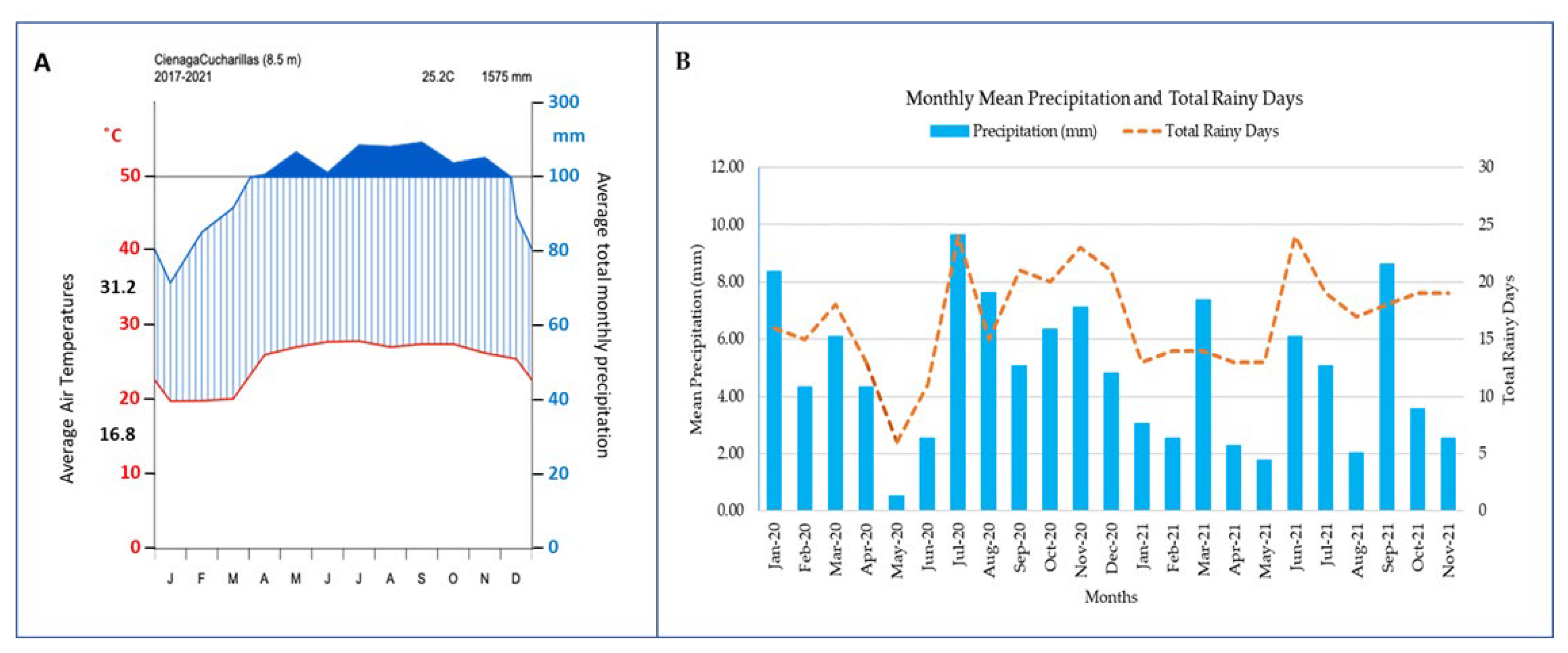
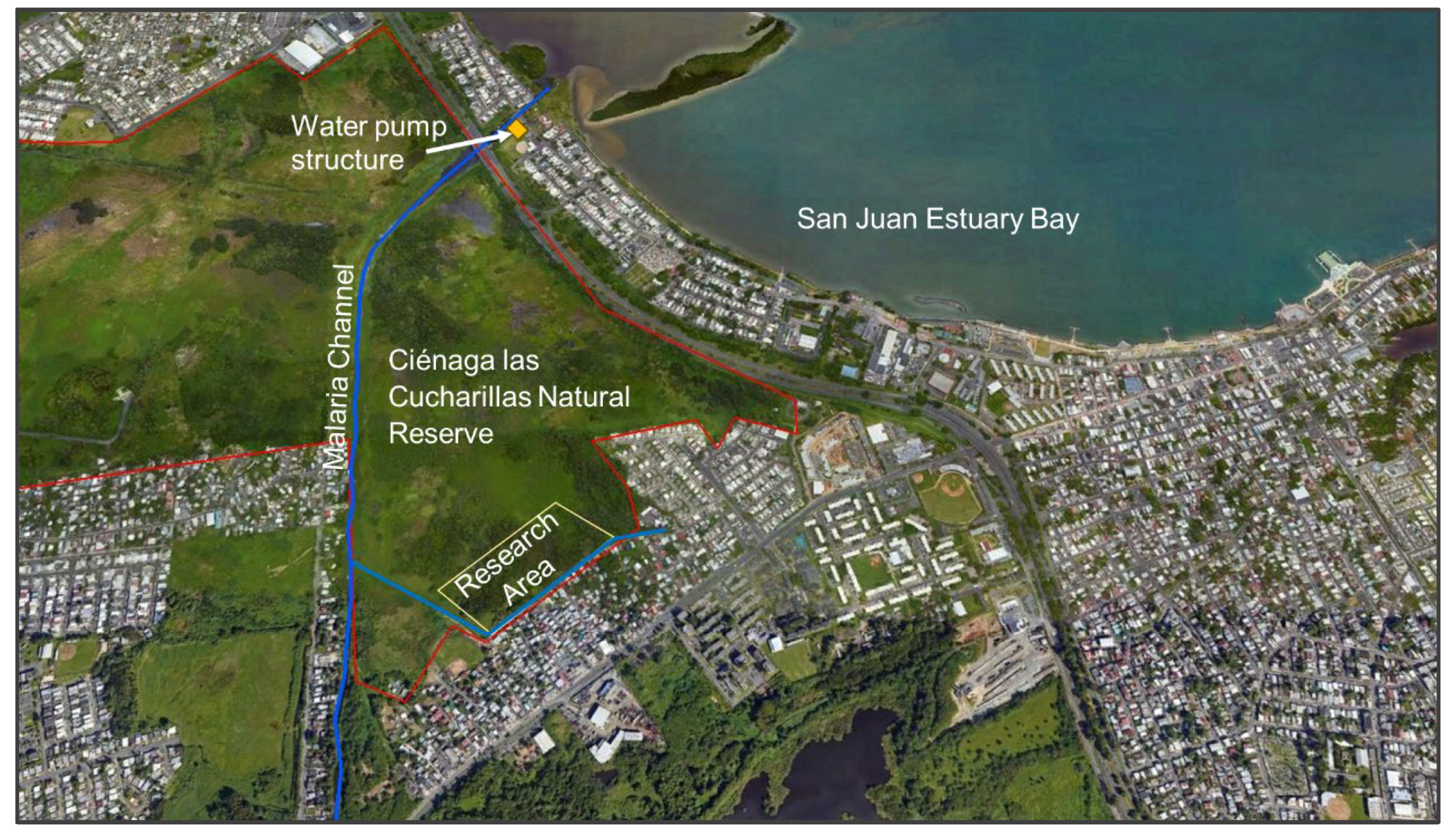
2.1. Study Area
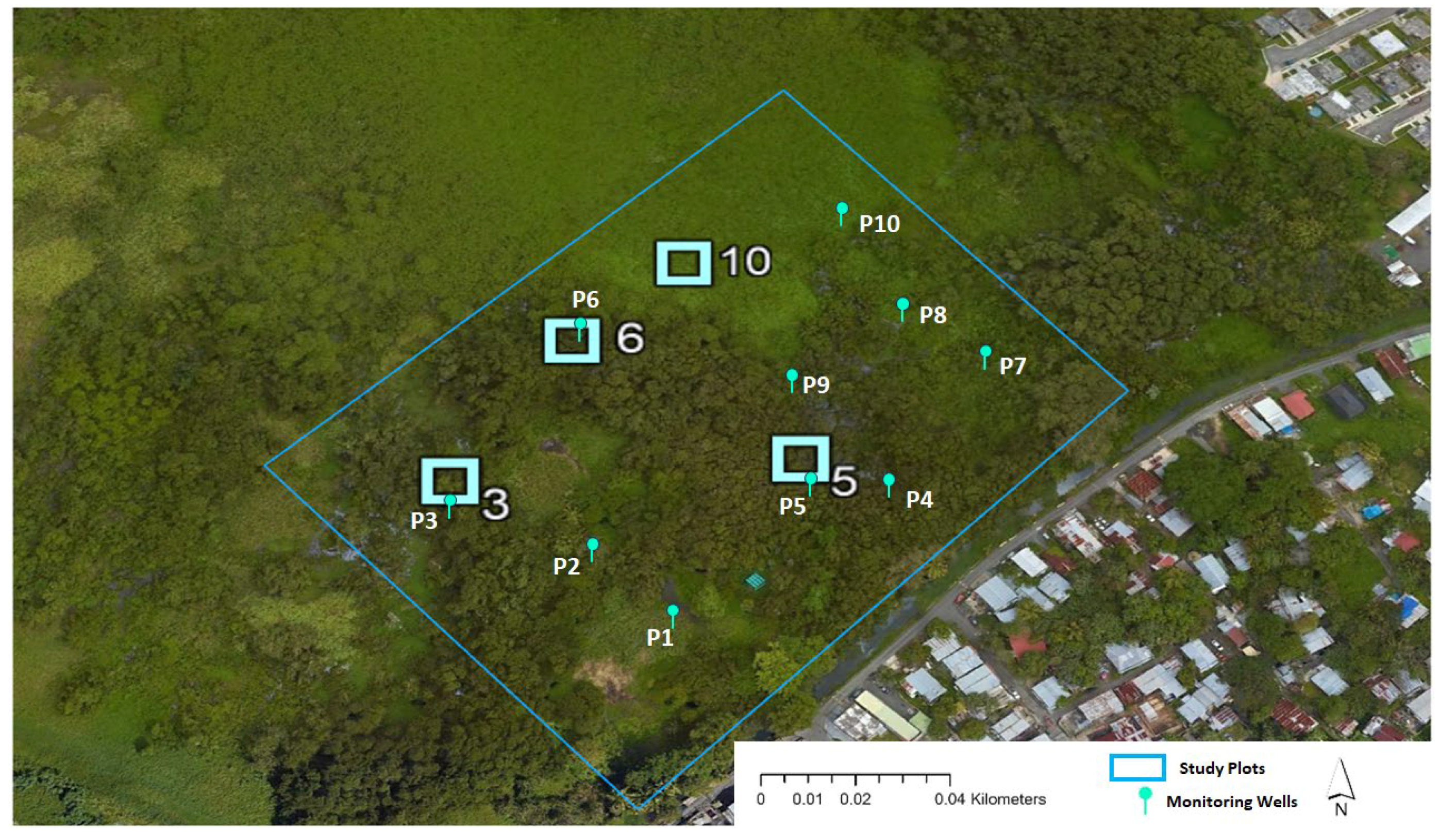
2.2. Research Area
2.3. Data Collection
2.4. Data Analysis
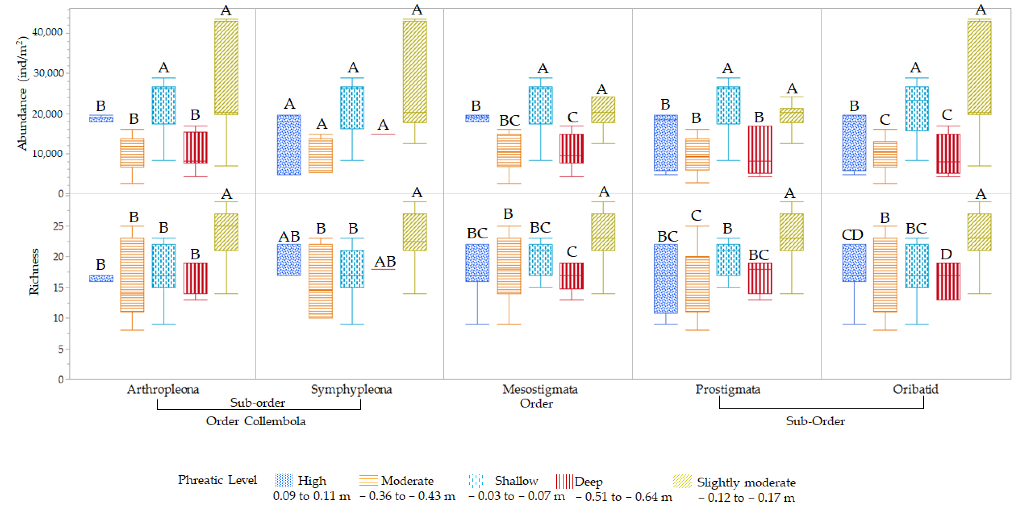
- High: 0.09 to 0.11 m
- Shallow/near surface: −0.03 to −0.07 m
- Slightly moderate: −0.12 to −0.17 m
- Moderate: −0.36 to −0.43 m
- Deep: −0.51 to −0.64 m
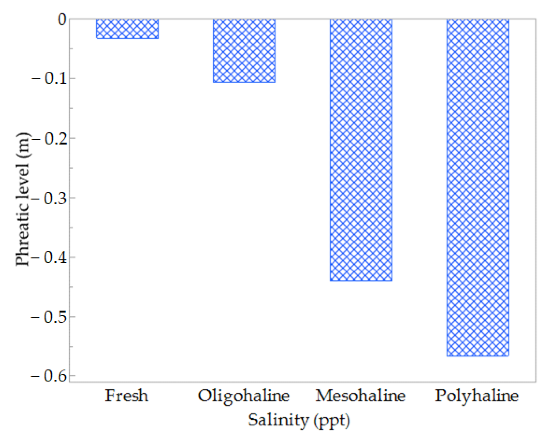
- Freshwater: 0 to 0.5 ppt
- Oligohaline: >0.5 to 5.0 ppt
- Mesohaline: >5.0 to 18.0 ppt
- Polyhaline: >18.0 to 33.0 ppt
3. Results
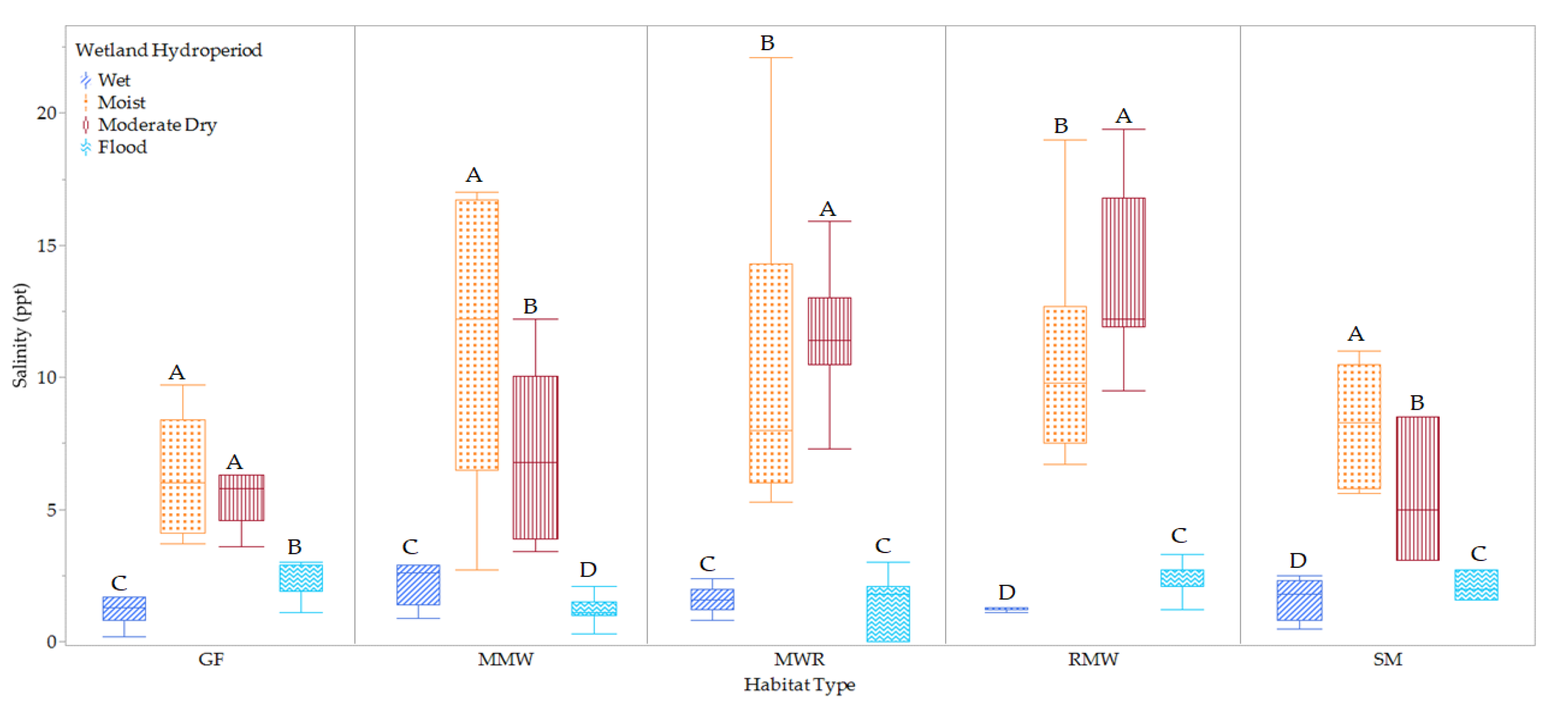
3.1. Variations in Habitat Phreatic Level and Salinity
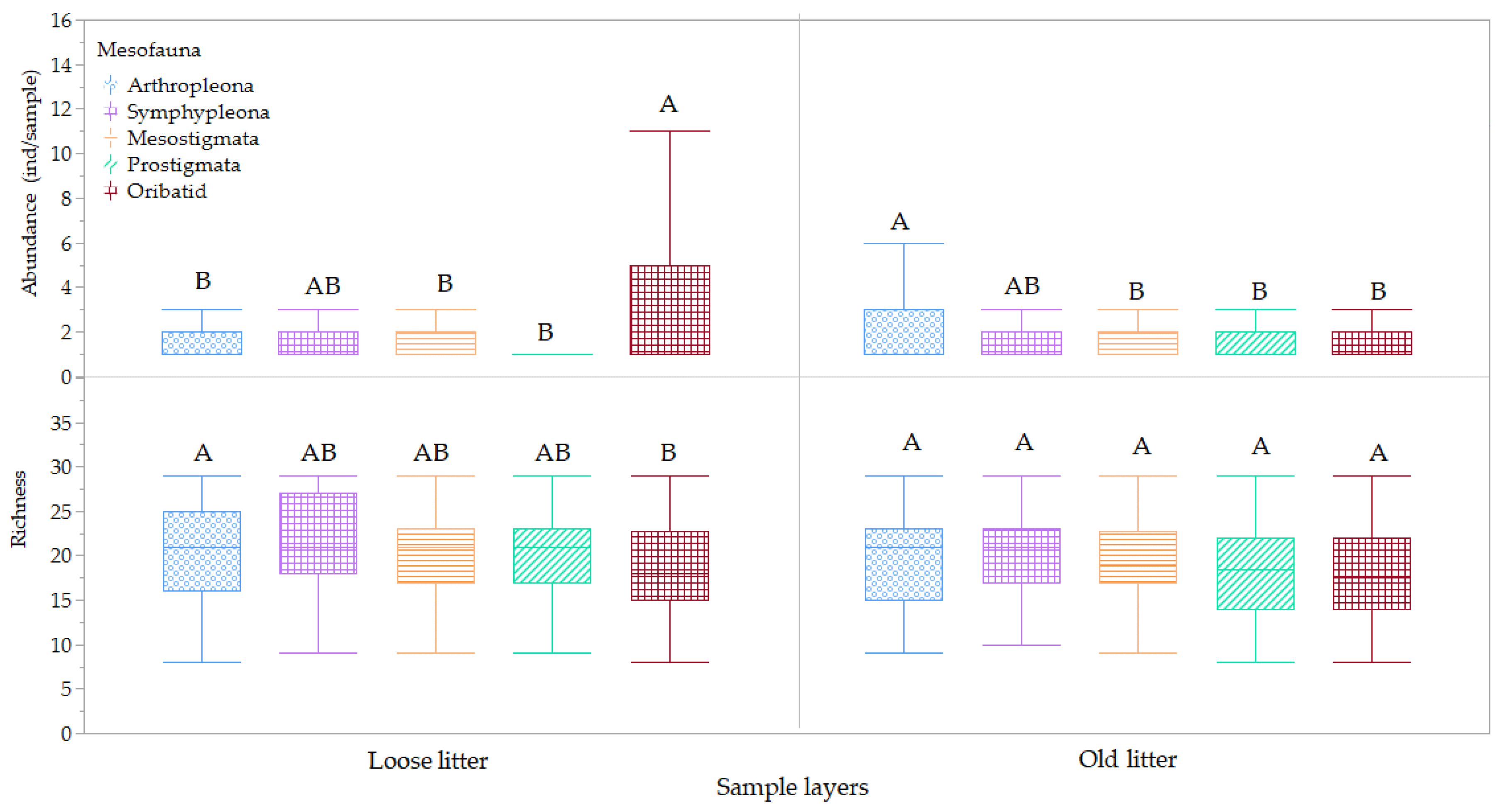
3.2. Mesofauna Diversity and Abundance between Habitat Types
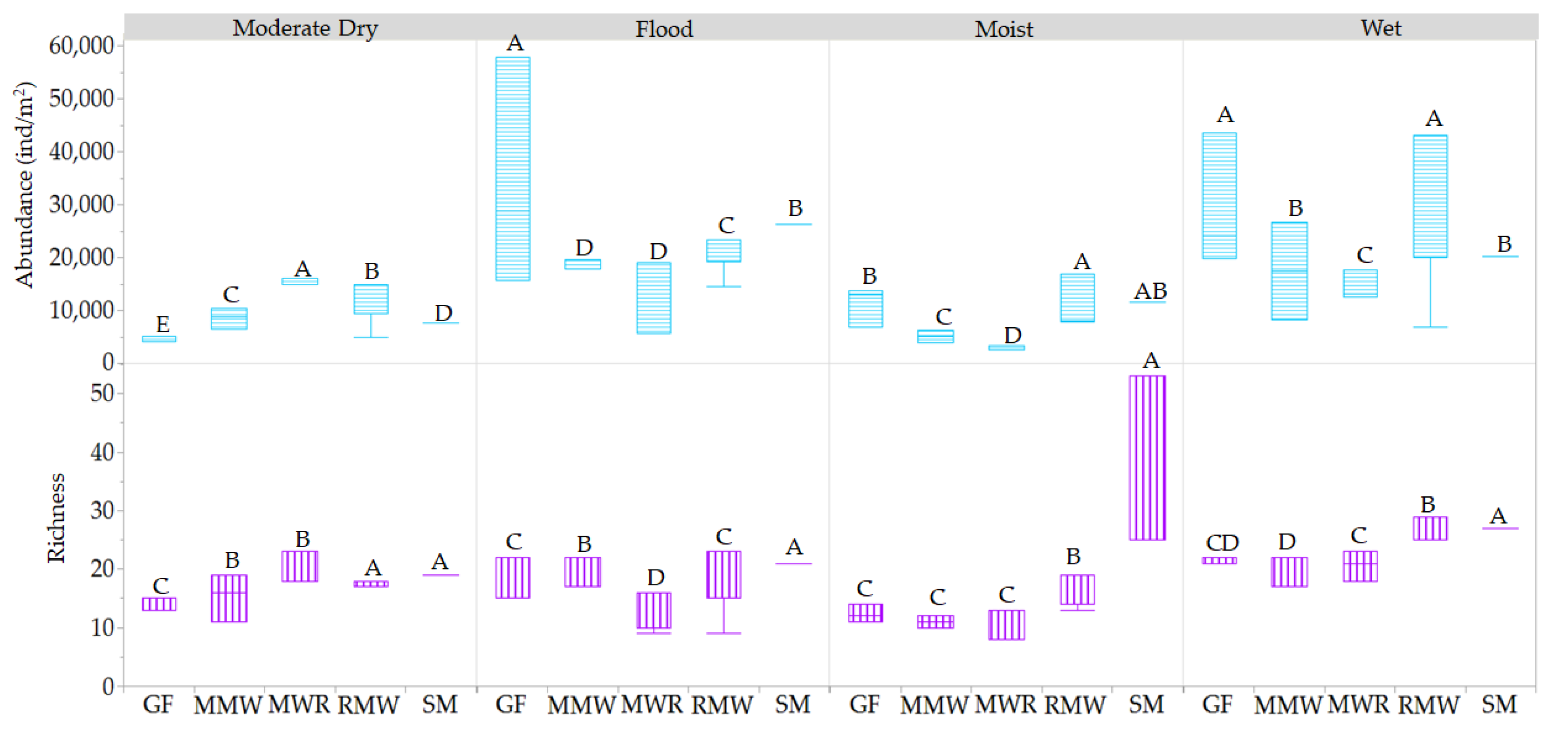
3.3. Influence of Hydroperiod Phreatic Level and Salinity on Mesofauna Diversity and Abundance
3.3.1. Hydroperiods
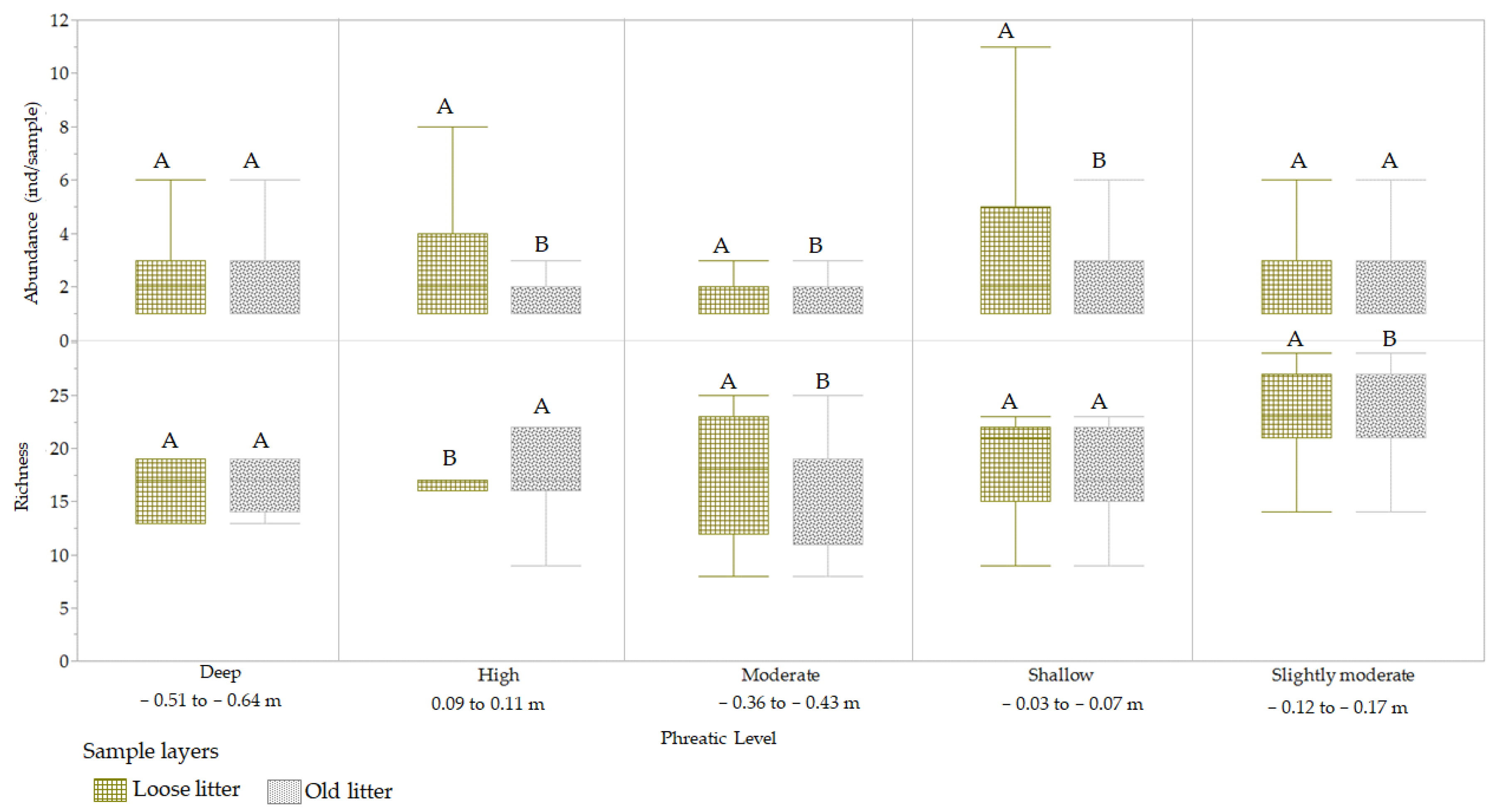
3.3.2. Phreatic Level
3.3.3. Salinity Conditions
4. Discussion
5. Conclusions
Author Contributions
Funding
Data Availability Statement
Acknowledgments
Conflicts of Interest
References
- Batzer, P.D.; Wu, H. Ecology of Terrestrial Arthropods in Freshwater Wetlands. Annual Reviews of Entomology 2020. Available online: https://www.annualreviews.org (accessed on 18 February 2022).
- Leonard, E.E.; Mast, A.M.; Hawkins, C.P.; Kettenring, K.M. Arthropod Assemblages in Invasive and Native Vegetation of Great Salt Lake Wetlands. Wetlands 2021, 41, 50. [Google Scholar] [CrossRef]
- Eckert, M.; Gaigher, R.; Pryke, J.; Samways, M.J. Soil arthropod assemblages reflect both coarse- and fine-scale differences among biotopes in a biodiversity hotspot. J. Insect Conserv. 2023, 27, 155–166. [Google Scholar] [CrossRef]
- Lavelle, P.; Decaëns, T.; Aubert, M.; Barot, S.; Blouin, M.; Bureau, F.; Rossi, J.P. Soil invertebrates and ecosystem services. Eur. J. Soil Biol. 2006, 42 (Suppl. S1), S3–S15. [Google Scholar] [CrossRef]
- Mulder, C.; Den Hollander, H.A.; Vonk, J.A.; Rossberg, A.G.; Jagers op Akkerhuis, G.A.; Yeates, G.W. Soil resource supply influences faunal size–specific distributions in natural food webs. Naturwissenschaften 2009, 96, 813. [Google Scholar] [CrossRef] [PubMed]
- Swift, M.J.; Heal, O.W.; Anderson, J.M.; Anderson, J.M. Decomposition in Terrestrial Ecosystems; University of California Press: Berkeley, CA, USA, 1979; Volume 5. [Google Scholar]
- Reilly, K.; Cavigelli, M.; Szlavecz, K. Agricultural management practices impact soil properties more than soil microarthropods. Eur. J. Soil Biol. 2023, 117, 103516. [Google Scholar] [CrossRef]
- Coleman, D.C.; Callaham, M.; Crossley, D.A., Jr. Fundamentals of Soil Ecology; Academic Press: Cambridge, MA, USA, 2017. [Google Scholar]
- Culliney, T.W. Role of Arthropods In Maintaining Soil Fertility. Plant Epidemiology and Risk Analysis Laboratory, Plant Protection, and Quarantine, Center for Plant Health Science and Technology, USDA-APHIS. Agriculture 2013, 3, 629–659. [Google Scholar] [CrossRef]
- Lavelle, P.; Blanchart, E.; Martin, A.; Martin, S.; Alister, S. A Hierarchical Model for Decomposition in Terrestrial Ecosystems: Application to Soils of the Humid Tropics. Biotropica 2013, 25, 130–150. [Google Scholar] [CrossRef]
- Wardle, D.A.; Bardgett, R.D.; Klironomos, J.N.; Setälä, H.; Van Der Putten, W.H.; Wall, D.H. Ecological linkages between aboveground and belowground biota. Science 2004, 304, 1629–1633. [Google Scholar] [CrossRef]
- Collins, W.W.; Qualset, C.O. (Eds.) Biodiversity in Agroecosystems; CRC Press: Boca Raton, FL, USA, 1998. [Google Scholar]
- Chaos of Delight. Soil Animals-Springtails, Soil Mites and Mesofauna. Available online: https://www.chaosofdelight.org/ (accessed on 25 July 2023).
- Menta, C.; Remelli, S. Soil health and arthropods: From complex system to worthwhile investigation. Insects 2020, 11, 54. [Google Scholar] [CrossRef]
- Socarrás, A. Mesofauna edáfica: Indicador biológico de la calidad del suelo. Pastos Y Forrajes 2013, 36, 5–13. [Google Scholar]
- Gerecke, R.; Krantz, G.W.; Walter, D.E. (Eds.) A manual of acarology (with contributions by V. Belan-Pelletier, D.R. Cook, M.S. Harvey, J.E. Keirans, E.E. Lindquist, R.A. Norton, B.M. OConnor and I. M. Smith), 3rd edn. Exp. Appl. Acarol. 2010, 52, 451–452. [Google Scholar] [CrossRef]
- Behan-Pelletier, V.; Lindo, Z. Oribatid Mites: Biodiversity, Taxonomy and Ecology, 1st ed.; CRC Press: Boca Raton, FL, USA, 2023. [Google Scholar] [CrossRef]
- Potapov, A.M.; Beaulieu, F.; Birkhofer, K.; Bluhm, S.L.; Degtyarev, M.I.; Devetter, M.; Goncharov, A.A.; Gongalsky, K.B.; Klarner, B.; Korobushkin, D.I.; et al. Feeding habits and multifunctional classification of soil-associated consumers from protists to vertebrates. Biol. Rev. Camb. Philos. Soc. 2022, 97, 1057–1117. [Google Scholar] [CrossRef] [PubMed]
- Capinera, J.L. Springtails (Collembola). In Encyclopedia of Entomology; Capinera, J.L., Ed.; Springer: Dordrecht, The Netherlands, 2008. [Google Scholar] [CrossRef]
- Lawton, J. Biology of springtails. Insecta: Collembola. By Stephen P. Hopkin. (Oxford: Oxford University Press, 1997). 344 pp. ISBN 0 19 8540484 1. Bull. Entomol. Res. 1998, 88, 106. [Google Scholar] [CrossRef]
- Kagainis, U.; Jucevica, E.; Salmane, I.; Ventins, J.; Melecis, V. Does Climate Warming Affect Soil Mesofauna? In Proceedings of the 2nd Global Soil Biodiversity Conference, Nanjing, China, 25 October 2017. Available online: https://www.researchgate.net/publication/320559698_Does_Climate_Warming_Affect_Soil_Mesofauna (accessed on 3 August 2022).
- Ghiglieno, I.; Simonetto, A.; Orlando, F.; Donna, P.; Tonni, M.; Valenti, L.; Gilioli, G. Response of the Arthropod Community to Soil Characteristics and Management in the Franciacorta Viticultural Area (Lombardy, Italy). Agronomy 2020, 10, 740. [Google Scholar] [CrossRef]
- Haarlov, N. Vertical Distribution of Mites and Collembola in Relation to Soil Structure. In Soil Zoology; Mc Kevan, D.K.E., Ed.; Butter Worths: London, UK, 1955; pp. 167–179. [Google Scholar]
- Bezemer, T.M.; Fountain, M.T.; Barea, J.M.; Christensen, S.; Dekker, S.C.; Duyts, H.; Van der Putten, W.H. Divergent composition but similar function of soil food webs of individual plants: Plant species and community effects. Ecology 2010, 91, 3027–3036. [Google Scholar] [CrossRef] [PubMed]
- Liu, Y.; Du, J.; Xu, X.; Kardol, P.; Hu, D. Microtopography-induced ecohydrological effects alter plant community structure. Geoderma 2020, 362, 114119. [Google Scholar] [CrossRef]
- Batzer, P.D.; Sharitz, R.R. Ecology of Freshwater and Estuarine Wetlands; The University of California: Berkeley, CA, USA, 2006. [Google Scholar]
- Kim, J.; Lee, J.; Cheong, T.; Kim, R.; Koh, D.; Ryu, J.; Chang, H. Use of time series analysis for the identification of tidal effect on groundwater in the coastal area of Kimje, Korea. J. Hydrol. 2005, 300, 188–198. [Google Scholar] [CrossRef]
- Hernández, E. Ecophysiological Responses of Plant Functional Groups to Environmental Conditions in a Coastal Urban Wetland, Ciénaga Las Cucharillas in Northeastern Puerto Rico; Ecolab, Department of Environmental Science, The University of Puerto Rico: San Juan, PR, USA, 2022. [Google Scholar]
- Krediet, A.F.; Ellers, J.; Berg, M.P. Collembola community contains larger species in frequently flooded soil. Pedobiologia 2023, 99, 150892. [Google Scholar] [CrossRef]
- Van Dijk, J.; Didden, W.A.; Kuenen, F.; van Bodegom, P.M.; Verhoef, H.A.; Aerts, R. Can differences in soil community composition after peat meadow restoration lead to different decomposition and mineralization rates? Soil Biol. Biochem. 2009, 41, 1717–1725. [Google Scholar] [CrossRef]
- Pereira, C.S.; Lopes, I.; Sousa, J.P.; Chelinho, S. Effects of NaCl and seawater induced salinity on survival and reproduction of three soil invertebrates species. Chemosphere 2015, 135, 116–122. [Google Scholar] [CrossRef]
- Batzer, D.; Wu, H.; Wheeler, T.; Eggert, S. Peatland invertebrates. In Invertebrates in Freshwater Wetlands; Springer: Cham, Switzerland, 2016; pp. 219–250. [Google Scholar] [CrossRef]
- IPCC. 2023: Climate Change 2023: Synthesis Report. In Contribution of Working Groups I, II and III to the Sixth Assessment Report of the Intergovernmental Panel on Climate Change; Core Writing Team, Lee, H., Romero, J., Eds.; IPCC: Geneva, Switzerland, 2023; pp. 35–115. [Google Scholar] [CrossRef]
- Filho, W.L.; Nagy, G.J.; Setti, A.F.F.; Sharifi, A.; Donkor, F.K.; Batista, K.; Djekic, I. Handling the impacts of climate change on soil biodiversity. Sci. Total Environ. 2023, 869, 161671. [Google Scholar] [CrossRef] [PubMed]
- Bardgett, R.D.; Yeates, G.W.; Anderson, J.M. Patterns and determinants of soil biological diversity. In Biological Diversity and Function in Soils; Cambridge University Press: Cambridge, UK, 2005; pp. 100–118. [Google Scholar] [CrossRef]
- Barberena-Arias, M.F.; Cuevas, E. Physicochemical Foliar Traits Predict Assemblages of Litter/Humus Detritivore Arthropods; InTech: Rijeka, Croatia, 2018. [Google Scholar] [CrossRef]
- Mazhar, S.; Pellegrini, E.; Contin, M.; Bravo, C.; De Nobili, M. Impacts of salinization caused by sea level rise on the biological processes of coastal soils—A review. Front. Environ. Sci. 2022, 10, 1212. [Google Scholar] [CrossRef]
- Wu, P.; Zhang, H.; Wang, Y. The response of soil macroinvertebrates to alpine meadow degradation in the Qinghai–Tibetan Plateau, China. Appl. Soil Ecol. 2015, 90, 60–67. [Google Scholar] [CrossRef]
- Wu, T.J. Effects of global change on soil fauna diversity: A review. J. Appl. Ecol. 2013, 24, 581–588. [Google Scholar]
- National Weather Service. Climatological Data for TOA BAJA LEVITTOWN, PR—Year 2020 to 2021. Available online: https://www.weather.gov/wrh/climate?wfo=sju (accessed on 9 September 2023).
- Kennaway, T.; Helmer, E.H. The forest types and ages cleared for land development in Puerto Rico. GIScience Remote Sens. 2007, 44, 356–382. [Google Scholar] [CrossRef]
- Pumarada-O’Neill, L. Los Puentes Históricos de Puerto Rico; Centro de Investigación y Desarrollo, Recinto de Mayagüez, Universidad de Puerto Rico: Mayagüez, PR, USA, 1991. [Google Scholar]
- Webb, R.M.; Gómez-Gómez, F. Synoptic Survey of Water Quality and Bottom Sediments, San Juan Bay Estuary System, Puerto Rico, December 1994–July 1995. In Water Resources Investigations Report; U.S. Geological Survey: Denver, CO, USA, 1998. [Google Scholar] [CrossRef]
- Cuevas, E.; (Ecolab, St. Paul, MN, USA); (University of Puerto Rico, San Juan, Puerto Rico). Personal communication, 2023.
- Branoff, B.; Cuevas, E.; Hernández, E. Assessment of Urban Coastal Wetlands Vulnerability to Hurricanes in Puerto Rico; DRNA: San Juan, Puerto Rico, 2018; Available online: http://drna.pr.gov/wp-content/uploads/2018/09/FEMA-Wetlands-Report.pdf (accessed on 3 August 2023).
- United States Department of Agriculture (USDA). NRCS Web Soils Survey. Ciénaga las Cucharillas. Available online: https://websoilsurvey.usda.gov/ (accessed on 16 June 2023).
- Chen, Y.; Wang, B.; Pollino, C.A.; Cuddy, S.M.; Merrin, L.E.; Huang, C. Estimate of flood inundation and retention on wetlands using remote sensing and GIS. Ecohydrology 2014, 7, 1412–1420. [Google Scholar] [CrossRef]
- Hernández, E.; (Ecolab, St. Paul, MN, USA); (University of Puerto Rico, San Juan, Puerto Rico). Personal communication, 2021.
- National Weather Service. Tropical Storm Isaias—29–31 July 2020. US Department of Commerce. National Oceanic and Atmospheric Administration. National Weather Service. Available online: https://www.weather.gov/sju/isaias2020 (accessed on 16 June 2023).
- National Weather Service. 21–23 August 2020. US Dept of Commerce. National Oceanic and Atmospheric Administration. National Weather Service. Available online: https://www.weather.gov/sju/laura2020 (accessed on 16 June 2023).
- Barberena-Arias, M.F. Single Tree Species Effects on Temperature, Nutrients, and Arthropod Diversity in Litter and Humus in the Guánica Dry Forest. Ph.D. Thesis, The University of Puerto Rico, San Juan, Puerto Rico, 2008. [Google Scholar]
- USDA Soil Quality Institute. Soil Quality Test Kit; Agricultural Research Service, Natural Resources Conservation Service: Washington, DC, USA, 1999. [Google Scholar]
- National Weather Service. Climatological Data for La Puntilla Station (ID Number 9755371), San Juan, Puerto Rico. 2021. Available online: https://www.ndbc.noaa.gov/station_page.php?station=sjnp4 (accessed on 16 June 2023).
- Herrera, F. Artrópodos del suelo como bioindicadores de recuperación de sistemas perturbados. Venesuelos 2003, 11, 67–78. [Google Scholar]
- Environmental Protection Agency. Chapter 14 of the Volunteer Estuary Monitoring Manual, A Methods Manual, 2nd ed.; Environmental Protection Agency: Washington, DC, USA, 2006; EPA-842-B-06-003. [Google Scholar]
- Zheng, X.; Wang, H.; Tao, Y.; Kou, X.; He, C.; Wang, Z. Community diversity of soil meso-fauna indicates the impacts of oil exploitation on wetlands. Ecol. Indic. 2022, 144, 109451. Available online: https://www.sciencedirect.com/science/article/pii/S1470160×22009244 (accessed on 17 March 2023). [CrossRef]
- Li, K.; Bihan, M.; Yooseph, S.; Methé, B.A. Analyses of the microbial diversity across the human microbiome. PLoS ONE 2012, 7, e32118. [Google Scholar] [CrossRef]
- Daghighi, E.; Koehler, H.; Kesel, R.; Filser, J. Long-term succession of Collembola communities in relation to climate change and vegetation. Pedobiologia 2017, 64, 25–38. [Google Scholar] [CrossRef]
- Kiernan, D. Natural Resources Biometrics. Open SUNY. Milne Library (IITG PI); State University of New York at Geneseo: Geneseo, NY, USA, 2014; Available online: https://open.umn.edu/opentextbooks/textbooks/205 (accessed on 4 June 2023).
- Cordes, P.; Maraun, M.; Schaefer, I. Dispersal patterns of oribatid mites across habitats and seasons. Exp. Appl. Acarol. 2022, 86, 173–187. [Google Scholar] [CrossRef] [PubMed]
- Walter, D.E.; Proctor, H.C. Life Cycles, Development and Size. In Mites: Ecology, Evolution & Behaviour; Springer: Dordrecht, The Netherlands, 2013. [Google Scholar] [CrossRef]
- Heydari, M.; Eslaminejad, P.; Kakhki, F.V.; Mirab-balou, M.; Omidipour, R.; Prévosto, B.; Lucas-Borja, M.E. Soil quality and mesofauna diversity relationship are modulated by woody species and seasonality in semiarid oak forest. For. Ecol. Manag. 2020, 473, 118332. [Google Scholar] [CrossRef]
- Barrios, E.; Sileshi, G.; Shepherd, K.; Sinclair, F. Agroforestry and Soil Health: Linking Trees, Soil Biota, and Ecosystem Services. Soil Ecol. Ecosyst. Serv. 2012, 14, 315–330. [Google Scholar] [CrossRef]
- Lugo, A.E.; Medina, E.; Cuevas, E.; González, O.R. Ecological and physiological aspects of Caribbean shrublands. Caribb. Nat. 2019, 58, 1–35. [Google Scholar]


| Plot | 3 | 5 | 6 | 10 | ||
|---|---|---|---|---|---|---|
| Micro-elevation | −0.79 | −0.72 | −0.86 | 0.1 | ||
| Habitat Type | Mangrove woodland (MMW) | Rehabilitated mangrove woodland (RMW) | Mangrove woodland (MWR) | >50 years Shrub (SM) | 6 years grass & ferns (GF) | |
| Stage | Mature | Rehabilitated; damaged by Hurricane Maria | Natural recolonization damaged by Hurricane Maria | Mature | Early successional | |
| % Cover Plants Species | 92.6% L. racemosa 3.2% Acrostichum sp. 4.2% grasses of the Poaceae family | 59.9% young and seedlings L. racemosa, 33.8% herbs and vines 4.2% grasses of the Poaceae family 2.0% Acrostichum sp. | 46.0% young and seedlings L. racemosa, 7.9% Acrostichum sp., 13.3% D. ecastaphyllum, 32.8% grasses of Poaceae family | 40.4% D. ecastaphyllum | 2.2% L. racemosa (young trees), 0.4% Acrostichum sp., 56.9% Echinochloa sp. | |
| Plant Type | Woody, fern, and grass | Woody, fern, herbs, and grass | Woody, fern, shrubs and grass | Shrubs | Woody, fern, and grass | |
| Soil Type | Mineral allochthonous embedded in an organic matrix (Martín Peña) | Organic (peat) Autochthonous (Saladar muck) | ||||
| Mean Salinity * | Wet Period | 3.4 ± 2 O | 2.8 ± 1 O | 2.4 ± 2 O | 2.1 ± 2 O | 2.1 ± 2 O |
| Dry Period | 4 ± 0.4 O | 12 ± 2 M | 11 ± 5 M | 7 ± 1 M | 7 ± 1 M | |
| Sampling Date | Sampling Time * | Tide (m) | Tide Description |
|---|---|---|---|
| 18 June 2020 | 7:00 | 0.22 | High |
| 10:00 | 0.05 | Low | |
| 25 June 2020 | 7:00 | 0.48 | High |
| 10:00 | 0.23 | Low | |
| 23 October 2020 | 7:00 | 0.31 | High |
| 10:00 | 0.14 | Low | |
| 19 March 2021 | 7:00 | 0.29 | High |
| 10:00 | 0.15 | Low | |
| 9 June 2021 | 7:00 | 0.22 | High |
| 10:00 | 0.10 | Low |
| Hydroperiod Phreatic Level (m) | |||
|---|---|---|---|
| Moderate Dry | Flood | Moist | Wet |
| −0.49 ± 0.06 D | −0.01 ± 0.07 A | −0.44 ± 0.12 C | −0.12 ± 0.03 B |
| Hydroperiod Phreatic Level (m) | ||||
|---|---|---|---|---|
| Habitats | Moderate Dry | Flood | Moist | Wet |
| GF | −0.51 B | −0.05 D | −0.36 A | −0.12 B |
| MMW | −0.41 A | 0.11 A | −0.43 B | −0.07 A |
| MWR | −0.41 A | 0.09 B | −0.36 A | 0.12 B |
| RMW | −0.54 C | −0.03 C | −0.64 C | −0.17 C |
| SM | −0.51 B | −0.05 D | −0.36 A | −0.12 B |
| Phreatic Level by Salinity | ||
|---|---|---|
| Habitats | Spearman ρ | Prob > |ρ| |
| GFM | −0.5 | <0.0001 |
| MMW | −0.8 | <0.0001 |
| MWR | −0.8 | <0.0001 |
| RMW | −0.6 | <0.0001 |
| SM | −0.7 | <0.0001 |
| Variable | By Variable | Spearman p | Prob > |p| |
|---|---|---|---|
| Richness | Phreatic Level | −0.5 | <0.0001 |
| Salinity (ppt) | 0.3 | <0.0001 | |
| Abundance (ind/m2) | Salinity (ppt) | −0.5 | <0.0001 |
| Phreatic Level | 0.5 | <0.0001 |
| Mesofauna Richness | Wald Chi-Squared | Prob > Chi-Squared | Mesofauna Total Abundance | Wald Chi-Squared | Prob > Chi-Squared |
|---|---|---|---|---|---|
| Habitat type | 658 | <0.0001 | Habitat Type | 568 | <0.0001 |
| Phreatic level | 472 | <0.0001 | Phreatic level | 260 | <0.0001 |
| Salinity | 57 | <0.0001 | Salinity | 12 | 0.0005 |
Disclaimer/Publisher’s Note: The statements, opinions and data contained in all publications are solely those of the individual author(s) and contributor(s) and not of MDPI and/or the editor(s). MDPI and/or the editor(s) disclaim responsibility for any injury to people or property resulting from any ideas, methods, instructions or products referred to in the content. |
© 2024 by the authors. Licensee MDPI, Basel, Switzerland. This article is an open access article distributed under the terms and conditions of the Creative Commons Attribution (CC BY) license (https://creativecommons.org/licenses/by/4.0/).
Share and Cite
Ortiz-Ramírez, G.; Hernández, E.; Pinto-Pacheco, S.; Cuevas, E. The Dynamics of Soil Mesofauna Communities in a Tropical Urban Coastal Wetland: Responses to Spatiotemporal Fluctuations in Phreatic Level and Salinity. Arthropoda 2024, 2, 1-27. https://doi.org/10.3390/arthropoda2010001
Ortiz-Ramírez G, Hernández E, Pinto-Pacheco S, Cuevas E. The Dynamics of Soil Mesofauna Communities in a Tropical Urban Coastal Wetland: Responses to Spatiotemporal Fluctuations in Phreatic Level and Salinity. Arthropoda. 2024; 2(1):1-27. https://doi.org/10.3390/arthropoda2010001
Chicago/Turabian StyleOrtiz-Ramírez, Gloria, Elix Hernández, Solimar Pinto-Pacheco, and Elvira Cuevas. 2024. "The Dynamics of Soil Mesofauna Communities in a Tropical Urban Coastal Wetland: Responses to Spatiotemporal Fluctuations in Phreatic Level and Salinity" Arthropoda 2, no. 1: 1-27. https://doi.org/10.3390/arthropoda2010001