Challenges and Solutions for Engineering Applications on Smartphones

Abstract

This paper starts by presenting the concept of a mobile application. A literature review is conducted, which shows that there is still a certain lack with regard to smartphone applications in the domain of engineering as independent simulation applications and not only as extensions of smartphone tools. The challenges behind this lack are then discussed. Subsequently, three case studies of engineering applications for both smartphones and the internet are presented, alongside their solutions to the challenges presented. The first case study concerns an engineering application for systems control. The second case study focuses on an engineering application for composite materials. The third case study focuses on the finite element method and structure generation. The solutions to the presented challenges are then described through their implementation in the applications. The three case studies show a new system of thought concerning the development of engineering smartphone applications.

1. Introduction

This paper focuses on defining the challenges in developing and implementing an engineering application on a smartphone platform.

An engineering application is a form of software that offers the user the ability to conduct operations and simulations related to an engineering domain. The use of desktop engineering applications has become a staple in all engineering fields and disciplines, such as P-spice in Electronics Engineering, AutoCAD in civil engineering, MATLAB in Control Systems Engineering, and others. However, engineering applications on smartphone platforms are still in their early stages and offer much lower levels of depth and simulation capability in comparison to their desktop counterparts. The objective of this work is to present the set of challenges that currently prevents smartphone-based engineering applications from reaching these levels, as well as presenting a working set of solutions to these challenges.

The importance of this work is due to the rapid increase in the widespread of smartphones in comparison to their desktop counterparts. According to the International Data Corporation, shipments of smartphones reached approximately 1.205 billion [1], whereas personal computer (PC) sales reached approximately 310 million [2]. Figure 1 [3] shows the differences in sales between desktops and smartphones in the period of 2019–2022. This increase in reach also shows an increase in dependency on smartphones for regular and daily activities beyond mobile services. Business intelligence estimated the value of in-store mobile payments in the USA at USD 128 billion in 2021 [4]. The accessibility of smartphones and their future potential have led researchers to study the possibilities of mobile technology in several domains, such as automating construction site monitoring [5]. As stated above, one of the younger and less-explored domains of smartphone applications is the field of engineering, as explored further in the literature review below. Current developments focus on smartphones’ hardware components or the smartphone as an outlet of connection, such as cloud-based simulations instead of smartphone-based simulations. One example is MATLAB Mobile, MATLAB’s mobile application, which connects the user to the Mathworks cloud, where all operations and data are sent from the mobile to the Mathworks server to be processed [6]. This, in turn, leads to limitations in innovation in such applications due to the development of the hardware/software in smartphones and the cloud. With the increase in system demand from simulations and modeling, engineering-based smartphone applications currently lag behind their PC counterparts in terms of advancement and innovation.

The methodology for the research presented in this paper begins with a literature review covering standard engineering-based smartphone applications. This is intended to show the level and depth of current standard engineering-based smartphone applications, as well as their current limitations. Subsequently, a set of challenges is conceptualized based both on the work of the authors on engineering-based smartphone applications (used later as case studies) and the limitations that were evident in the applications shown in the literature. The applications developed by the authors are used as case studies to offer a functional presentation of the solution to each of the explained challenges. While not all the challenges are present in all of the developed applications, the challenge that was most evident in each concerned application is addressed. The contribution of this research is in the provision of a set of potential challenges that should be considered from the start of the development of an engineering-based smartphone application alongside a solution example, which, in turn, will allow future work to efficiently bypass these challenges.

This paper starts by defining the concept of the mobile application in Section 2 and then discusses the literature surrounding engineering-based smartphone applications in Section 3. Next, the challenges are discussed in Section 4. Case studies are then introduced to present real-time solutions to the challenges described. The listed applications are smartphone-based and web-based. The first case study, in Section 5, concerns smartphone applications for systems control. The second case study, in Section 6, focuses on a smartphone application for composite materials. The third case study, in Section 7, is a smartphone application using the finite element method. The aim is to show a detailed solution to each of the challenges.

2. Mobile Application Concept

The term “application” is used for all electronic platforms and includes both smartphones and desktops. In simple terms, an application is a program that is intended to serve a specific purpose. A mobile application is designed to run on mobile devices which include smartphones and tablets [7]. The two most known Operating Systems (OS) for smartphones are Android and Mac OS, but several other Operating Systems have been developed [8]. Figure 2 [9] shows the components of a standard mobile application architecture.

The Presentation Layer is the front end of the application and represents the main connection between the user and the application. It is composed of the User Interface (UI) elements and the related parts [10]. The Business Layer contains the defined business entities alongside the workflows and holds the main connection between the front end and the back end of the application [11]. The Service Layer is composed of the service interfaces where data is translated between the business layer and external data contacts [12]. The Data Layer is formed of the data utilities and the data accessed components [13].

Smartphone application tools can be classified into two categories: native mobile application tools (XCode, Android Studio, App Code, etc.) and cross-platform mobile application development tools (Xamarin, Ionic, React Native, etc.). The latter category allows the development of an application to be deployed for several platforms.

In broader terms, mobile applications are similar to desktop applications. However, it is through the analysis of this definition that a smartphone application would differ from standard desktop applications in several aspects other than technical.

To start on the technical side, desktop applications are developed on the same targeted platform, i.e., via other desktop applications, whereas smartphone applications are not developed on smartphones but on desktops alongside the use of emulators and simulators in order to design and test the application [14].

In addition, the nature of the usage of smartphones dictates that applications are highly preferred to be fast with low downtime and quick results. Smartphone users might tend to switch around between several applications that are constantly running in the smartphone background unlike in the case of desktop applications where such are usually intended to be solely used for a longer period of time. The varying usage types can lead to different performance and resource costs for the same application depending on the given scenario [13].

3. State of the Art

The main increase in engineering dependency has been mostly apparent in field service engineering domains. This advancement is backed by the constantly developing digital technology features that come with smartphones such as the different sensors, smart camera Artificial Intelligence (AI), and others [15]. Application prototypes are constantly being developed and marketed in order to test the reaction of engineers in the concerned fields [16]. The following state of the art aims to explore the fields that have shown a major increase in smartphone dependency.

3.1. Building Information Modeling (BIM)

BIM is a digital representation of a building and its internal features. It contains intelligent construction components that can include data attributes and parameter rules per item as shown in Figure 3 [17]. BIM offers consistent and coordinated views alongside a representation of the 3D model that is supported by a reliable 4D representation, which is time, and 5D data, which is the cost for design, construction, and operation of built assets. These features have been widely praised for their advancement and operation [18]. This modeling process has attracted worldwide attention in Architecture, Engineering, Construction, and Resource Management as there is growing evidence that adopting BIM increases efficiency and productivity [19]. BIM architecture management and editing tools are widely used in conflict detection, model and location communication, and planning. Some of the notable BIM smartphone applications include AR Mapper, Revizto, ARKi, and BIMx.

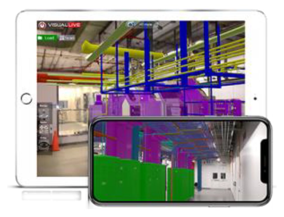
3.2. Augmented Reality (AR)

This technology first appeared in the fields of retail, travel, entertainment, social communication, and advertising but its increased affordability and ease of use has made the implementation of the technology in industry fields like the construction industry more feasible and approachable [20]. One of the important benefits observed is the possibility of reducing the time and cost behind explanation and design description, which hinder the efficiency of conducting value-adding tasks. Related studies show a generally low effectiveness rate on explanation and description tasks [21]. Recent AR applications use different tracking configurations that can be categorized into ‘mark-based’ and ‘marker-less’ types [22]. AR implementation is still a relatively new field in construction but some applications have already been present such as GAMMA AR, Morpholio AR, and DAQRI Smart Helmet.

3.3. Data Acquisition of Projects

A study from 2012 in the USA showed that 87% of subcontractors and 93% of the general contractors sampled were utilizing mobile devices on job sites in order to boost productivity [23]. Commercial applications have been developed in order to improve construction monitoring alongside detailing progress on the site. One example of such is ‘Site Progress’ which is designed to work with a database that is developed using the Asta Powerproject software.

3.4. Measurement and Data Collection

Smartphones have already built-in sensors that can be used for scientific measurements where they can be considered a multi-functional tool such as in magnetometry for detecting safe electromagnetic devices [24]. Other uses include tacheometry and telemetry. An example of this is the work of Dong-Hoon P. et al. [25], which aims to build an application that aids in the identification of a Volatile Organic Compound (VOC). This is through the collection of the standard testing paper result through the cellphone camera and the identification of the gas by analyzing the visual results with the application’s database. Another example of this is the work of Angela M. et al. [26], which introduces a smartphone-based instructional particle image velocimetry educational tool for Android that is open source and low cost. The concerned work offers users guided instruction that is backed by the technological infrastructure that allows them to visualize and study authentic flow fields in real time.

In addition to data measurement, smartphones can be used as widespread pinpoint devices for conducting wide surveys and mass data collection because of their large popularity and ease of carry. An example of such usage is in meteorology where a smartphone network can be implemented to monitor tropospheric delays and variations based on the changes in data collected by smartphone sensors [27].

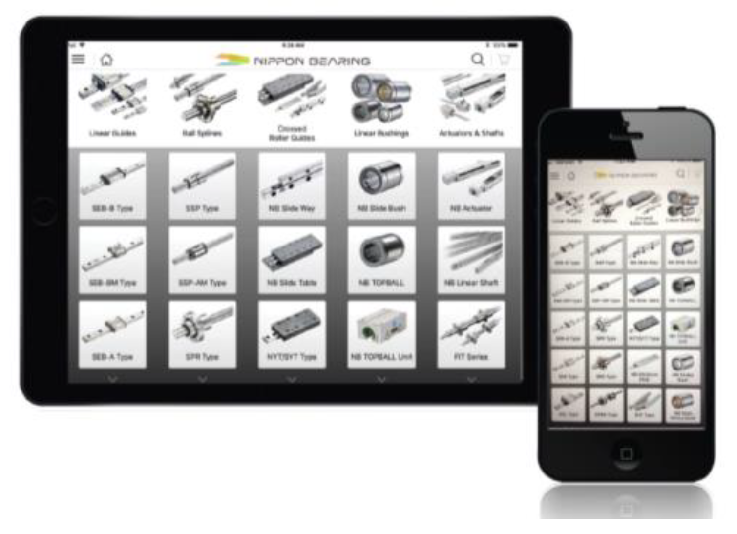
3.5. Computer-aided Design

CAD represents the technology that is related to the implementation of computer systems to assist in the creation, analysis, and modification of a design. With the increase in development and complexity of smartphones, CAD mobile applications have seen a rise after a somewhat shaky start [28]. Figure 4 [29] shows a developed CAD application for medical sensors and devices. While several known desktop CAD applications like AutoCAD have introduced their smartphone version, several other new applications are present such as Infinite Design, cadTouch, A360, and eDrawing.

3.6. Computer-aided Manufacturing (CAM)

Computer Aided Manufacturing can be seen as the use of computer-based systems in order to manage, plan, and optimize the operations of a manufacturing plant through a given computer interface. Simulation design and analysis are conducted with the aim to acquire insight into these complex systems, testing new methods of operations or resource policies and new concepts before implementing them as seen in Figure 3. The main benefit would be gathering the knowledge and information without disturbing the actual system or wasting resources, time, and cost [30].

An example of this is the Arduino mobile application that can connect the user to an Arduino printed circuit board (PCB) via their smartphone through a WAN connection. Other manufacturing applications on the smartphone platform include Manufacturing 360, Lean App, and Manufacturing MRP.

3.7. Discussion about Engineering Smartphone Applications

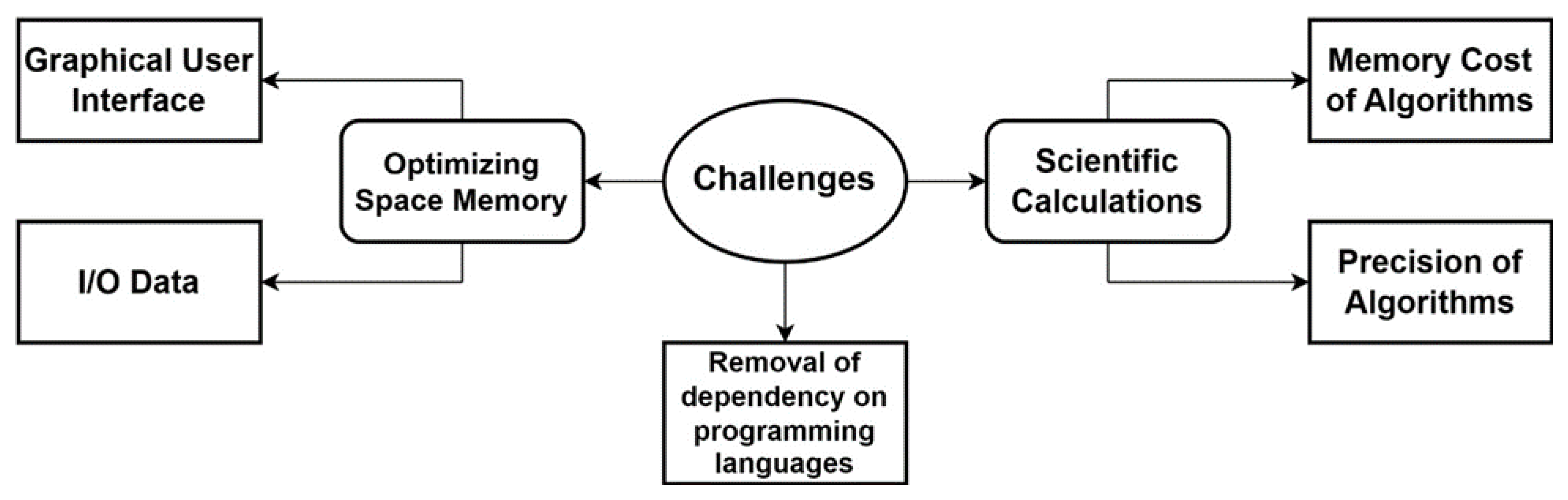
The examples and work shown above vary between several domains and fields. However, they share several similarities. For instance, a large portion of them heavily relies on the use of one or several of the smartphone’s sensors and other hardware features mainly the camera. The related smartphone components are the central point of operations, and the software/simulation to accompany it is secondary or just an attachment to the main operation. The work shown highlights the smartphone as a primary tool for measurement with less focus on computing and simulation. In addition, the presented state of the art might not completely encompass all of the recorded and published work and research, but most of which has been brought to light in recent years. Therefore, it is apparent that there is a certain lack in the density of research surrounding the topic despite a previous surge of interest in the earlier years. The relatively small amount of research can be contributed to several factors such as the increase in investment in cloud computing, the rapid development of smartphone capabilities or others. Thus, as stated before, scientific smartphone applications are mainly being developed with the focus on smartphones as being a compact set of tools all in one device, or as a visual enhancement to the camera’s input as it is seen with augmented reality, or as portals for desktop work such as blueprints and designs. However, research related to utilizing the smartphone’s computing capacities for simulation is still small and young if not nonexistent. With the lack of proper direct work towards smartphone scientific applications for simulation, any work that is related is seen through the introduction of new algorithms that replace old ones with the same efficiency and output. This is accompanied by computing less and memory requirements such as the introduction of less-demanding iterative methods for standard-used direct methods that are more demanding. It is to be noted that the reliance on the hardware development of smartphones to be able to accommodate more demanding simulation applications might not be feasible because desktop applications have shown to be advancing in requirements at a faster capacity. While smartphones are less likely to fully replace desktops in use and purpose, a large portion of scientific concepts and methods can be developed to remove the need for desktops for support.

4. Challenges

While other challenges are present and can influence the success of the development of the smartphone scientific calculation, the following have been found as the main challenges for implementation and development. Figure 5 shows the challenges in the discussion. They are primarily the result of the smartphone’s limited memory capacity, which leads to the impact of these challenges on smartphones where a large portion of them tend to be tolerable on desktop platforms.

4.1. Optimizing Space Memory

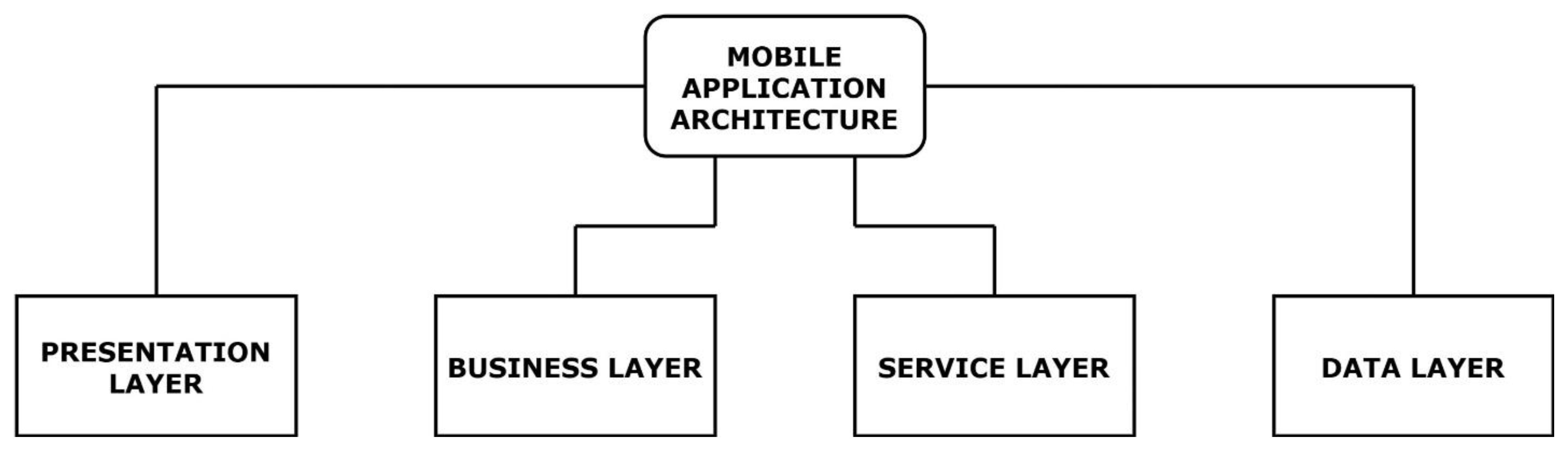
4.1.1. User Graphical Interface

Graphical User Interfaces (GUI) in scientific applications tend to be heavy in performance demands because of the standard amount of information and data that needs to be displayed to the user and manageable by the user. Unlike other applications, scientific applications mostly have a unique and dedicated interface for each application because of the difference between their respective fields. This is apparent in the variation between the research and published work throughout the different domains such as in spectral analysis [31], radiogenomic studies [32], agriculture [33], and others. Concerning mobile applications in general, the scientific study of usability guidelines for mobile applications is still young in development. Most of the conventional guidelines are based on common attributes between established mobile applications [34]. Despite the risks of increasing memory costs, UI studies and developments are generally designed with user preferences and tendencies as the highest priority [35]. An efficient User Interface offers the basis for improving the overall performance of the system [36]. A proper balance must be found between user satisfaction and memory costs where the latter must not heavily compromise the first. Several high-quality applications in the market have not gathered sufficient popularity due to complexity and an unattractive or confusing User Interface [37].

4.1.2. Data Management for Input/Output

Scientific applications tend to rely on a large set of input and output data for simulation and execution. E. Deelman et al. [38] show the difference in data management demands between standard applications and scientific applications because of the data-intensive nature of scientific workflow in these applications. While this cost can be negligible on desktop platforms because of the standard large space available, it becomes far more noticeable on smartphone platforms [39]. This is also noticeable because of the large amount of memory and disk space occupied by built-in systems and applications [40]. The optimization of saved data does not only improve disk space costs but the efficiency of access to this data [41]. In addition, the work of A. Carroll et al. [42] highlights the direct relation between storage size and energy consumption on smartphone platforms.

4.2. Scientific Calculations

4.2.1. Memory Cost of Algorithms

Scientific algorithms can lead to a large increase in complexity and memory costs for execution. Complexity results from the large and increasing scale of operations and simulations. A common example of this is matrix inversion. M. Ataeeshojai et al. [43] and M. Albreem [44] show the complexity challenges in matrix inversion despite modern computing. The cited work addresses the complexity issue on desktops which would be more staggering on smartphones. An algorithm’s performance varies based on external and internal factors. External factors usually vary between platforms and software whereas internal factors are related to the efficiency of algorithms both in memory space usage and time [42]. The potential cost of complex algorithms has led to research that focuses on mitigating the impact. An example of this is Shared-memory Parallelism [45].

4.2.2. Precision of Algorithms

A large portion of the standard algorithms used in scientific calculations are approximation algorithms where the output has a provable guarantee on the distance of the returned solution to the optimal one [46]. Approximation algorithms are commonly used in optimization problems where problems cannot be solved exactly in polynomial time. While iterative algorithms optimize memory costs, their implementation can result in increased runtime. This increase is due to the linear execution of operations [44]. In addition, standard iterative algorithms can have varying output efficiency based on the scenario and environment of execution. A common example of this in algorithm execution is Least-squares Method (LSM). Several methods derived from LSM include Partial-least Squares (PLS) and Regularized-least Squares (RLS) with each having varying performance results based on the given scenario. PLS run time is slower than other methods and is only efficient when variable number are more than compound numbers in the data set [47] and RLS is more efficient only when the coefficients are penalized or else it has more run time for same efficiency [48]. This example highlights the importance of the given scenarios and parameters on the performance of the employed algorithm.

4.3. Removal of Dependency on Programming Languages

Programming language compilers are costly on memory because of the compiler’s limited knowledge of the runtime execution of the compiled program [49]. In addition, non-optimized written codes can remove the consistency guarantees of the program both on memory cost and runtime [50]. The evolution in the domain of programming languages has been first observed by the transition from text-based language towards the implementation of Model Transformation Language (MTL) [51]. Model transformations are considered the basis of model-driven engineering (MDE), and dedicated MTLs emerged with the popularity of the MDE paradigm. MTLs claim to increase the ease of development of model transformations by abstracting from recurring transformation aspects and hiding complex semantics behind a simple and intuitive syntax. Nonetheless, MTLs are rarely adopted in practice, and thus there is still no empirical evidence for the claim of easier development [52]. In addition, implementing MTL does not remove the major requirement of programming languages which is skill, experience, and a deep knowledge of the meta-models involved [53]. User knowledge and skill can directly impact memory costs because of the risk of non-optimized written codes. Therefore, dedicated programming languages on smartphones are not common on the platform because of the high memory costs as well as the resulting disadvantages. For such reasons, the challenge is not to adopt the same concept of programming languages on the smartphone platform but to simply provide its advantages, which are mainly the customization possibilities they provide. In addition, the presented customization possibilities should also account for the scalability potential that is offered with the use of programming languages, therefore allowing the customization of both the details and size of the targeted projects.

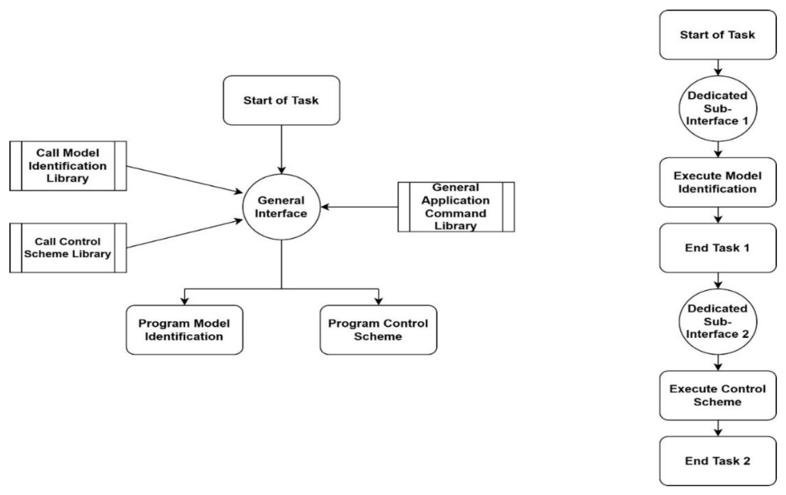
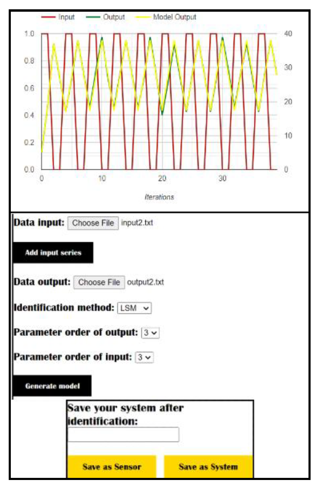
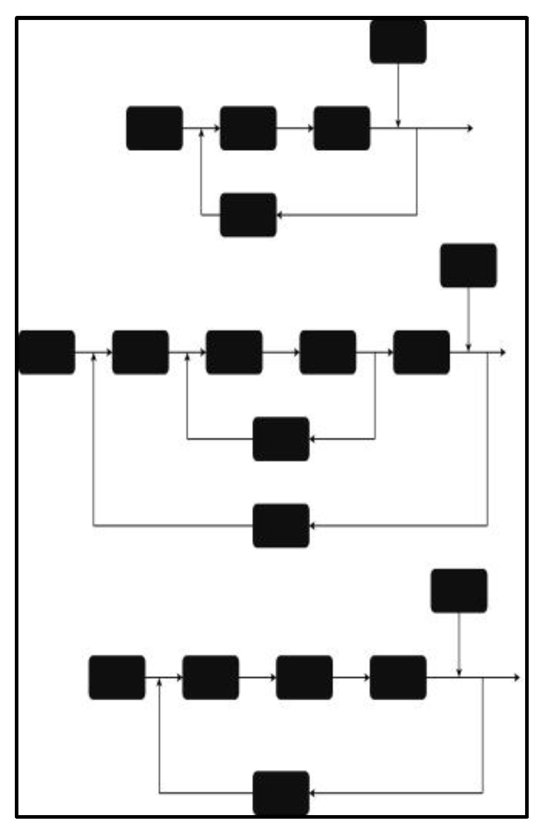
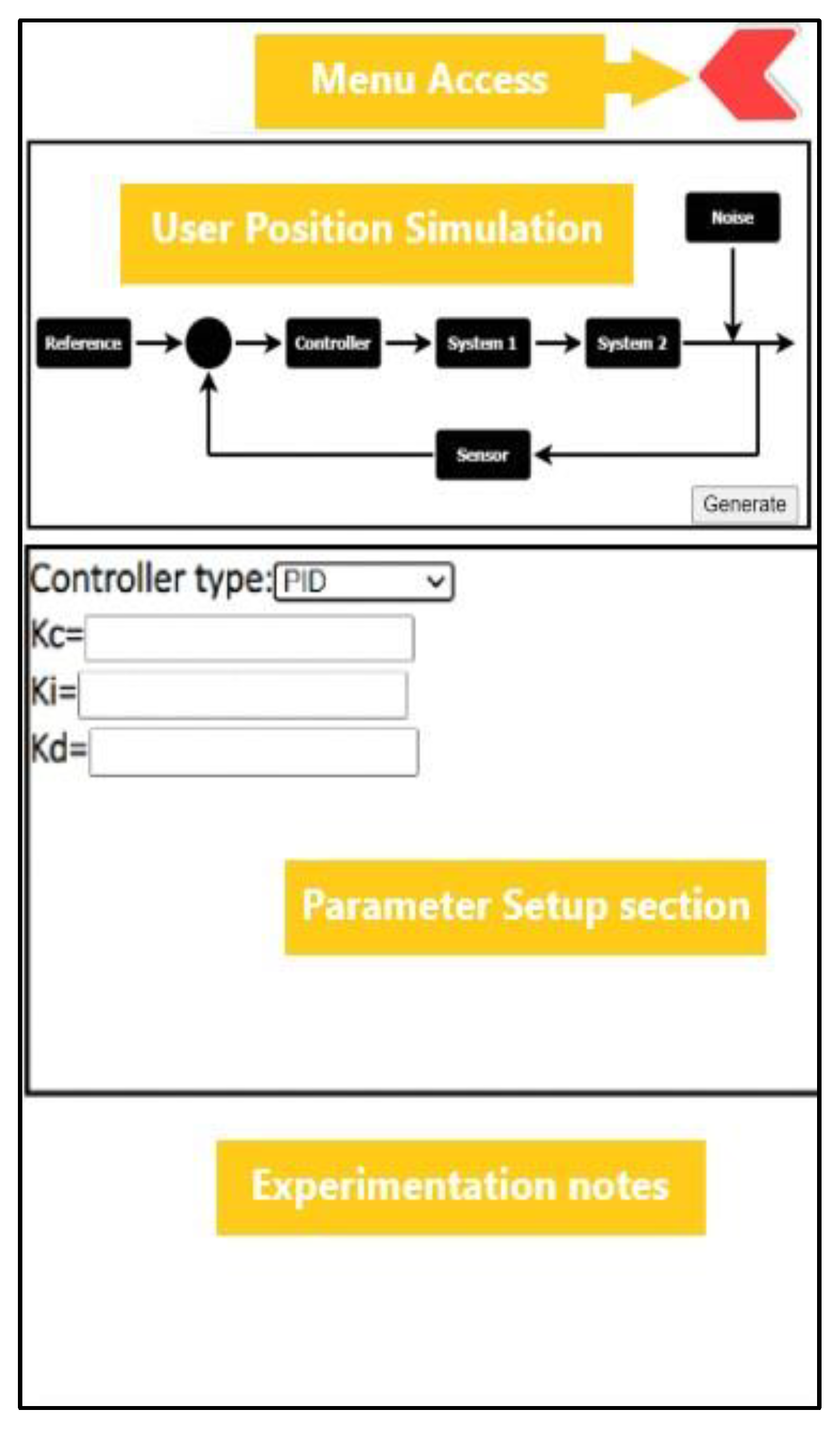
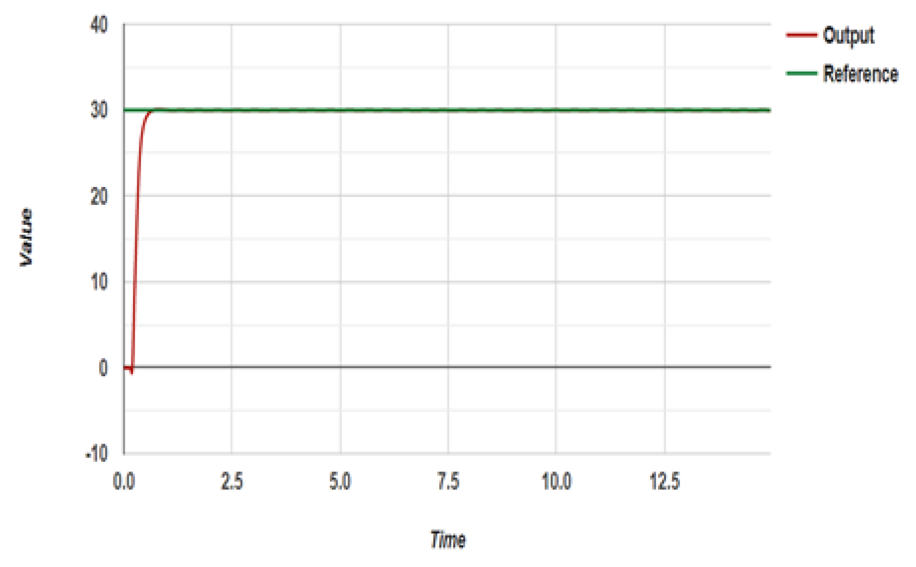
5. Case Study: Engineering Application for Systems Control

5.1. Concept

A smartphone application for control simulation is an application that accepts the data that is collected by any given system after the input and output of the system are collected where a model is identified for the system via model identification. Afterward, the resulting model is implemented in a control block diagram to be tested for control. The user sets up the proper sensors, controllers, feedback models, and other parameters. Other important aspects of system study are included such as stability testing, Bode diagram, state-space form, and others. Therefore the result would be a full-scale simulation from data measurement to control all through the smartphone. As discussed again later, current large-scale control simulations and methods are designed based on heavy hardware/software capacity, which is mainly found in computers and servers which highly surpass smartphone capabilities. Thus, the concept of the application in discussion cannot only rely on the currently known methods but a new set of methods and ideas need to be introduced in order to satisfy the smartphone constraints.

5.2. Proposed Solution

Two main challenges were present in the development of this application: the first concerning the GUI and the second concerning the removal of dependency on programming languages. These challenges are mainly due to the range of parameters, options, and data that are generally abundantly present in the domain of systems control.

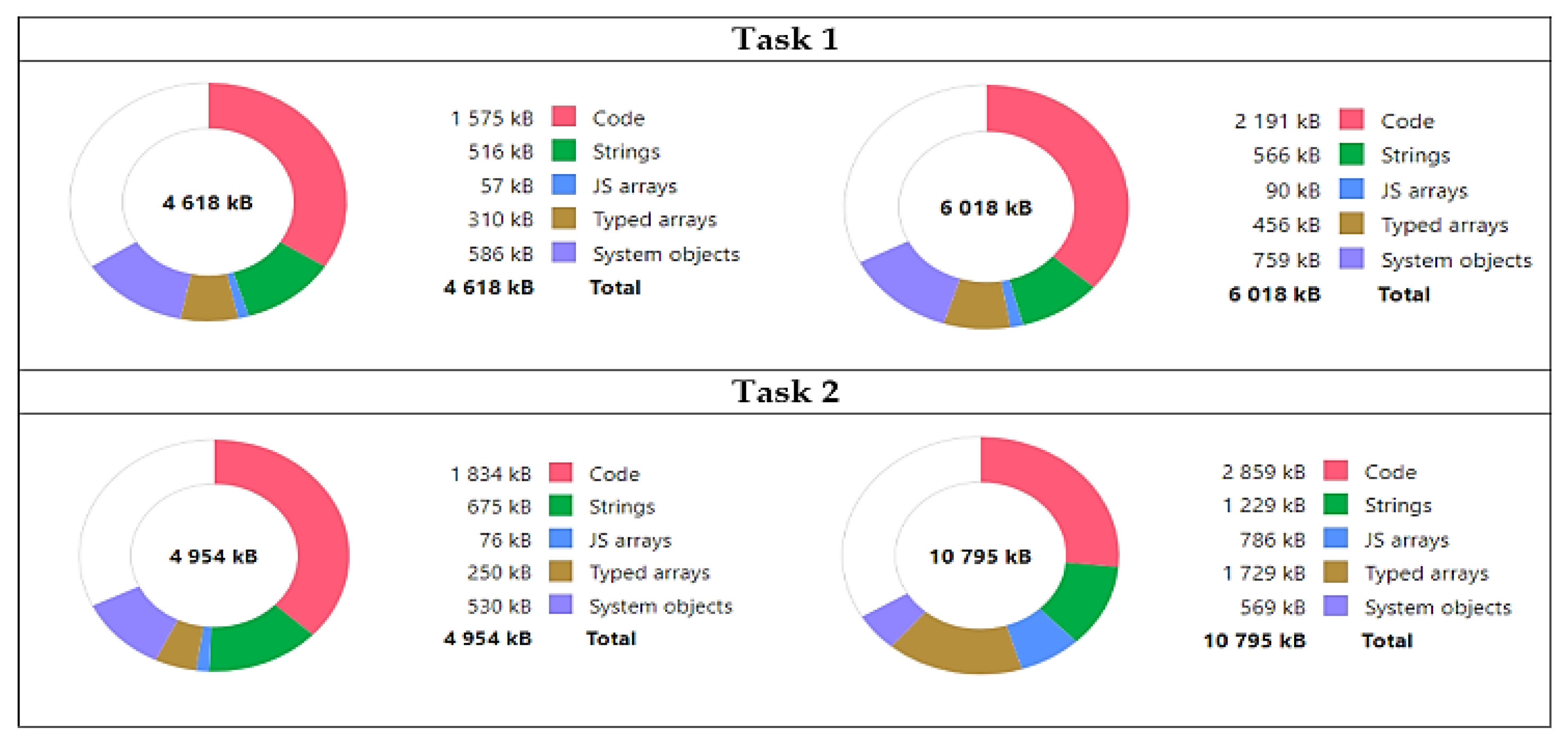
5.2.1. Challenge: Optimizing Space Memory for User Graphical Interface

This solution is based on the design of the used toolbox that enables the implementation of a varied set of dedicated sub-interfaces that spreads the tasks between sequentially connected and separated interfaces. In addition, the step-by-step filtering of the data to be used and methods reduce the memory costs behind simultaneously displaying and utilizing all of the resources needed. From the application’s side, this filtering can be applied not just to the possible options but also to the mathematical method choice as well. Moreover, sequential filtering would allow the application to execute smaller operations between each step. This decreases the number of operations conducted in the final execution and, therefore, splitting memory cost over the entirety of the process and not conducting all operations in one execution. This solution can be further explained by examining a task that is handled in a conventional interface and then in the proposed interface. The concerned task is to identify a system through model identification and then design and execute the control process. The difference between the 2 interfaces is shown in Figure 6.

In the conventional interface, all of the libraries and tools for the 2 tasks are present. The user cycles between the given options and commands in order to design the execution of the 2 given tasks. The output of task 1 and that of task 2 are simultaneously displayed for the user; therefore, increasing after task-execution memory cost as well.

In the proposed interface, the tasks are distributed on 2 dedicated sub-interfaces. Only the libraries used by the task are called and presented in the concerned sub-interface alongside the tools. After the execution of Task 1, the progress is saved to be used in the second sub-interface after the memory cost of the first sub-interface is cleared. Figure 7 details the memory costs both before Task 1 execution and after its execution and the same data for Task 2.

Figure 7 shows that the maximum after-execution memory cost of the 2 tasks is 10.795 MB. This is in comparison to the minimum memory requirements of other standard known scientific applications for control (MATLAB: 4 GB; Labview: 4 GB; Wolfram Mathematica: 4 GB) and after taking into consideration possible future scaling and worst-case-scenarios for the costs of the proposed solution.

5.2.2. Challenge: Removal of Dependency on Programming Languages

The removal of the need for programming languages dictates that the application should be providing all of the customization options and scenarios for systems control. Considering the large range of customization in control, the approach is to start from a general or major parameter and then move towards its own options and parameters. An example of the user experience during a task is presented in Figure 8.

The main task is to identify a model based on the data of an observed system and to design and test the control process of the obtained model. During the first step of model identification, the user is provided with a list of options for the method of model identification alongside the type of the resulting model. Each option is followed by a list of its parameters as well such as the number of input parameters and output parameters for the chosen model type. Afterward, the user saves the system and moves on to the control process. The same customization potential is presented. The user first starts by choosing the general design of the control process which is based on a broad range of standardized and conventional designs. The user then proceeds to customize the parameters of each block of the control scheme. Same as before, each block option chosen is followed by a subset of options and parameters to choose and tune. An example of this is the controller type choice; a chosen proportional–integral–derivative (PID) type controller presents the user with the Kp, Ki, and Kd parameters. Optional components are provided as well. An example of this is the ability to add noise to the system, whether it is Gaussian, Poisson or another, or to not have any type of noise. While the applications aim to provide all of the possible combinations and design options, this task is considerably staggering in systems control because of the large set of combinations and possible scenarios. For such reasons, the success of this approach relies on the knowledge and research capabilities of the developer and designer in the concerned domain.

5.3. Application

The example used to show the applications consists of identifying a DC servo system and its control process. The first step is the identification of the parameters by uploading the input and output, choosing the desired regressive model and the parameter number. This step is shown in Figure 9. Afterward, the user saves the system for control study later on. The user can also study the system further such as stability testing, Unit Step Response, Nyquist, and others. In the control study section, the user first chooses the controller type and moves on to choose the system to be studied and the remaining characteristics such as sensor, noise, the desired reference, and the controller characteristics. Several scheme customization options are provided in order to offer the user the potential to scale and fully customize concerned projects. Figure 10 shows the built-in control design options offered to the user. Figure 11 shows the User Interface and the associated toolbox to the left that allows the user to cycle between the different blocks of the control scheme. Figure 12 shows the output display.

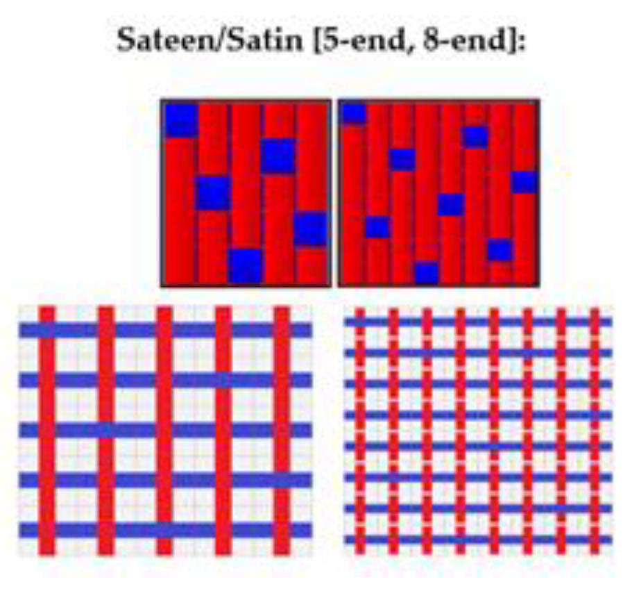
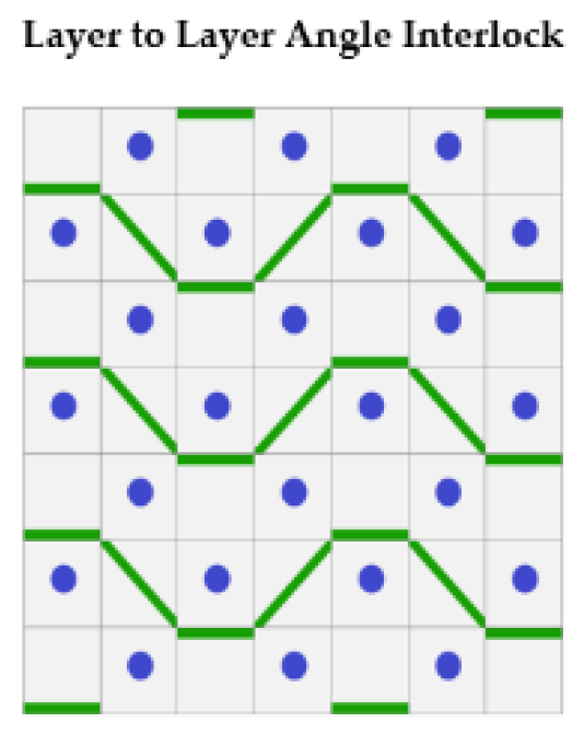
6. Case Study: Engineering Application for Composite Materials

6.1. Concept

The internal geometry of fabric reinforcement is an important factor in strengthening and reinforcement performance during composite production and service life of composite materials. When a 2.5 or 3D composite component is affected, the reinforcement is disabled in place (compressed, stretched, and sheared), and any model that defines the internal geometry of the reinforcement must undergo this modification. The code presented in this paper uses a general definition of the internal structure of the fabric reinforcement at the cell unit level, combined with the flexible and deformed models of UD—2D, 2.5D, and 3D woven, interlock, sandwich, and laminates. It is integrated with the modeling of resin flow, micro-mechanical calculations of properties of textile-based composites, and micro–macro analysis of composite parts, finite element models, and virtual reality software. This section describes this family of models, using an integrated description of the geometry of the reinforcement unit cell. It also summarizes these developments, with the aim of facilitating its future use of fabric models compiled by other researchers.

The general definition of the internal structure of the fabric reinforcement has been improved in K.U. Leuven. It is the final result of a development that began in the mid-1990s, with Vandeurzen et al. [54,55] on woven fabric composites and Gommers et al. [56]. Both authors are based on the definition of the internal geometry of the fabric in empirical data in the orientation of the thread, obtained by optical or electron microscopical detection on dry textiles and on the cross-section of textile composite. The main drawback of these early models was their reliance on strongly defined definitions of the inner geometry of the fabric. A major step forward can be reached when working with S.V. Lomov, who designed the 2D- and 3D-weaves internal geometric model (the CETKA model [57]), based on a small number of topological data (weaving style, inter-yarn distance) and yarn mechanical properties.

A further step was the full integration of geometric models with other speculative and predictive models suitable for combination analysis and performance prediction. Permeability tensors can be predicted by mimicking the flow of resin by reinforcement [58]; homogenized mechanical properties and local stress and strains can be performed by micro-mechanical calculations of composite structures [54] and can be linked to micro–macro composite analysis of composite components [55], finite elements models [59] and virtual reality software [60]. All of these models use an integrated geometric definition of the reinforcement unit cell.

The WiseTex and Texgen software package is widely used in the standard modeling of textile mesh structures and woven composite [61]. Incorporated with resin flow models, weft-knit and non-crimp warp-knit fabrics and laminates, thermodynamics, and micromechanical woven material counting. It is safe to say that there are a few other ways to build a visual sample for finite element analysis (FEA). Said et al. [62] proposed a Voronoi tessellation novel to create a virtual model of contrasts and heterogeneous material. Blacklock et al. [63] used the Monte-Carlo reconstruction algorithm based on the construction of the Markov series to produce a virtual sample.

6.2. Proposed Solution

The first main challenge present here was the memory cost of I/O data management. This is because of the density of the graphical components that form the output of the application. The second challenge concerns the removal of dependency on programming languages. This challenge is because of the range of elements and options included in the domain of composite material.

6.2.1. Optimizing Space Memory for I/O Data Management

The application Texgen is used here as a standard point of comparison and a staple of the conventionally used applications in this field.

There are two versions of the executable available: texgen-3.x.x.exe and texgen-bundle-3.x.x.exe. TexGen requires the Python interpreter to be installed in order to run. The standard installation package named texgen-3.x.x.exe does not include Python and the Python interpreter must be preinstalled manually. The installation package comes with the Python interpreter which means that no separate Python installation is required, as shown in Figure 13.

In Figure 13, the texgen-bundle-64bit-Python27-3.12.2.exe is up to 33.9 MB and texgen-Python27-3.12.2.exe is 25.6 MB. The required space to install the program is up to 100 MB. Moreover, from version 3.6.0, the default Windows download is the 64-bit version so there is no 32-bit format. On the other hand, the user can download the application discussed here [64] with less than 8 MB of space memory. The chosen format for saving is data files that contain data from multiple data sources, such as Microsoft Access and SQL Server databases. They are paired with a corresponding .dat file, which contains the project data schema and object information. Due to their tab-delimited format, data files may be imported into Microsoft Excel once their header information is stripped. A DAT file is a data file that contains specific information about the program used to create it. This file always has the .dat file extension, which is a generic format that can contain any information—video, audio, PDF, and virtually any other type of file. Many desktop and mobile apps reference DAT files, so these files would have the .dat extension. And there are many other cases where you might encounter these files. For video, audio, PDF, and other types of files, you need to open them with relevant apps such as media players, Adobe Reader, and so on.

A user can now open all kinds of .dat files on mobile phones just by using an application called “.dat file opener”. This app is the appropriate tool that allows the user to achieve this. It is also a cool dat file converter for Android and it is free to download. First, download “.dat file opener” from Play Store. Second, click on the install button to install the app on the phone. Third, open the newly installed app and click on the select file button and select your required .dat file. Finally, the content of your .dat file would be displayed on the screen. As mentioned earlier, the user can record all the information at any stage. Where the user can save the information about the fiber and its properties or construct the puzzle as in the case of 2D and 2.5D, and can even save the results and modify them. At any given time, the user can restore this data, update it, and continue its work.

Previous examples were calculated or structured and saved for the user to load them and use them at any time. Next, the file “interlock expmpl1” will be loaded.

Figure 14 shows an incomplete project made by the author to demonstrate the ability of the save and load feature that does not take up any large space, which is ideal for mobile applications and its uses, and shows a great tendency to easily use. Each color (green, blue) displays a different fiber type that is previously set. On the other hand, to work on any module today, such as TexGen, after the hard installation process and with its unavailability on mobile apps, the user is obliged first to create an AutoCAD drawing with all its complexity, time-consuming, storage memory needed and unable to simplify the work by a click and drop user-friendly way such as the author’s work. So, this kind of software is complex to use because it requires specific training and is expensive because it takes a long time to develop. It also requires significant computing power to manage fine simulation models and representatives.

The potential benefit of the current code lies in its ability to allow the fabrication of the textiles model from the fabrication of the textile fabric to its solution, which includes the production of mesh made using an integrated writing method, thus requiring much less human time and memory storage than conventional finite element models. The suggested hypothesis is the simplest that can be applied for determining the engineering data with all required information, and specifications from the user are presented in a “user-friendly” form that can make studying and searching a new level of excitement and interactivity. As shown in the Methodology section, applying the algorithm is easy and simple. All this research can be accessed easily with all its codes and models, along with its regulations and explanations needed. Working on these codes will eliminate the hard work caused by the computational efforts using software such as ABAQUS, Ansys, etc.

6.2.2. Challenge: Removal of Dependency on Programming Languages

This section aims to show the list of customization options offered by the application in order to remove the need for programming languages. In each category, the user should choose the subcategory if it exists. For example, in the laminate category and ABD sub-category (the matrix that describes the connection between the applied loads and the associated strains in the laminate), the user should specify the number of plies for the laminate composite material, for the number of plies is a key parameter of the ABD matrix. Then, after specifying the number of plies (let us say 3), the user has to fill in the mechanical properties by clicking on the filling parameter button, and, finally, the user submits the input parameters and the results should be shown automatically. As for the sandwich composite category and sandwich subcategory, for example, the user should specify the number of plies for each upper and lower skin of the sandwich composite and fill in the parameters. Finally, for the categories such as 2D fabric and interlock, the first step is to identify the dimensions of the structure by the user. The next step is building the puzzle after designing the composite structure and the code will run the tests to check if the structure is geometrically valid or if there is structural error. The user should fill in the engineering data, submit the values and the results shall appear automatically. Figure 15 shows the separate elements offered in the engineering application for composite materials. These elements are combined by the user in order to form the final design.

6.3. Application

This section provides a guide to the production of real-time fabric specimens, needed for the most reliable imitation and simulations. Virtual specimens are then created using advanced simulation techniques such as experimental calculations. In the last step, a virtual representation of the textile geometry is constructed in geometrical modeling code, in comparison with WiseTex software as shown in Figure 16 and Figure 17, where the first image set in each figure shows the result in WiseTex software and the grid image shows the result in the application in question. Figure 18 shows the building process after designing the composite structure. Each color (red, blue) shows a different fiber type that is preset.

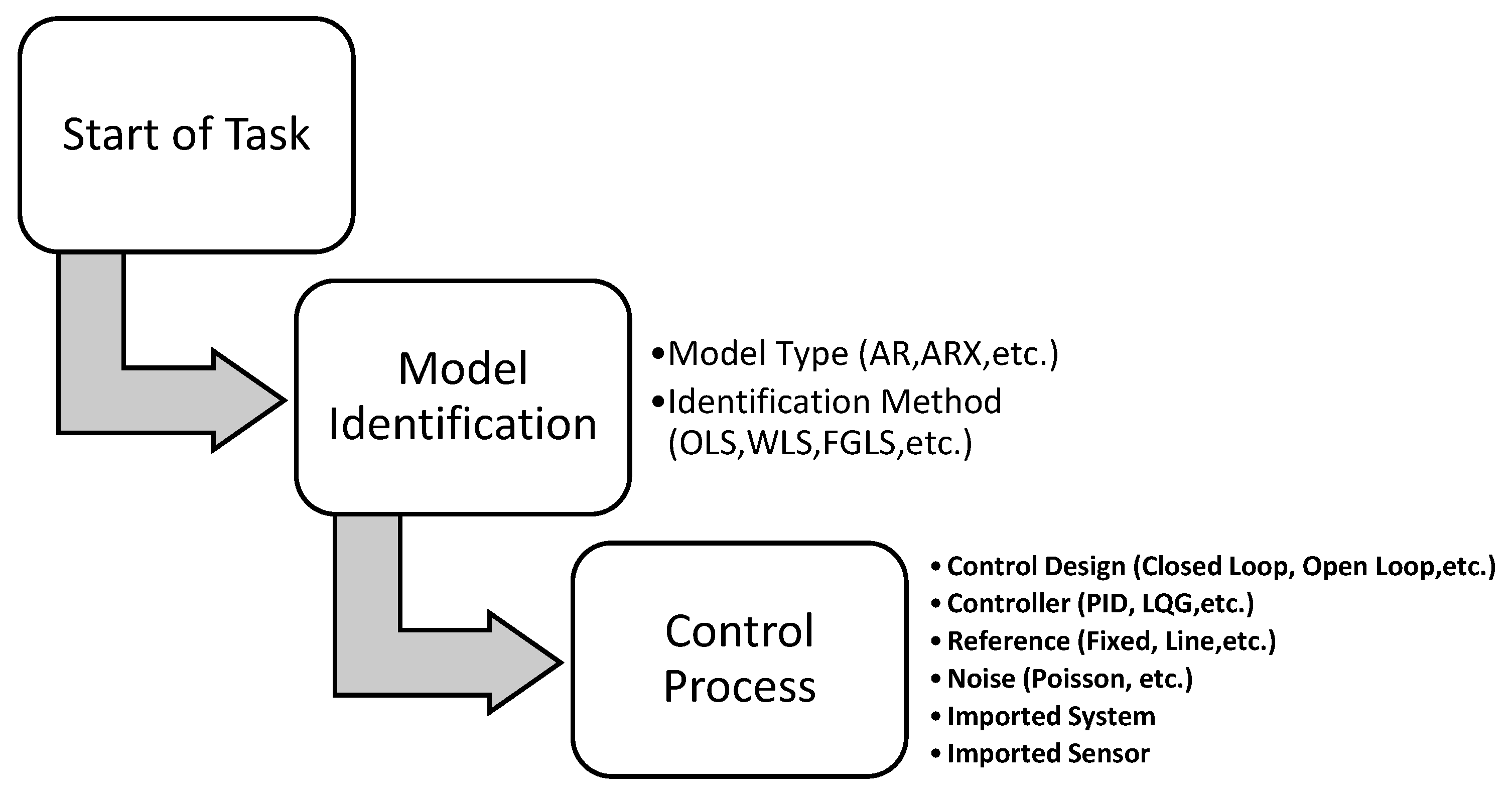
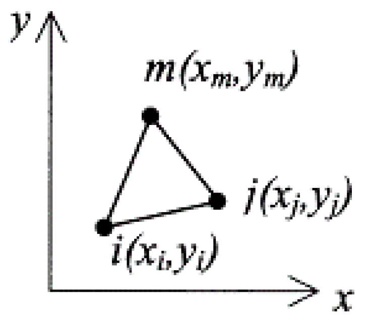
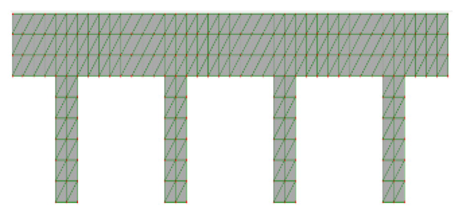
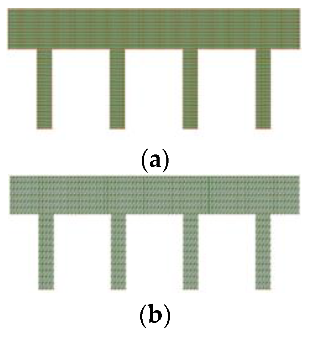
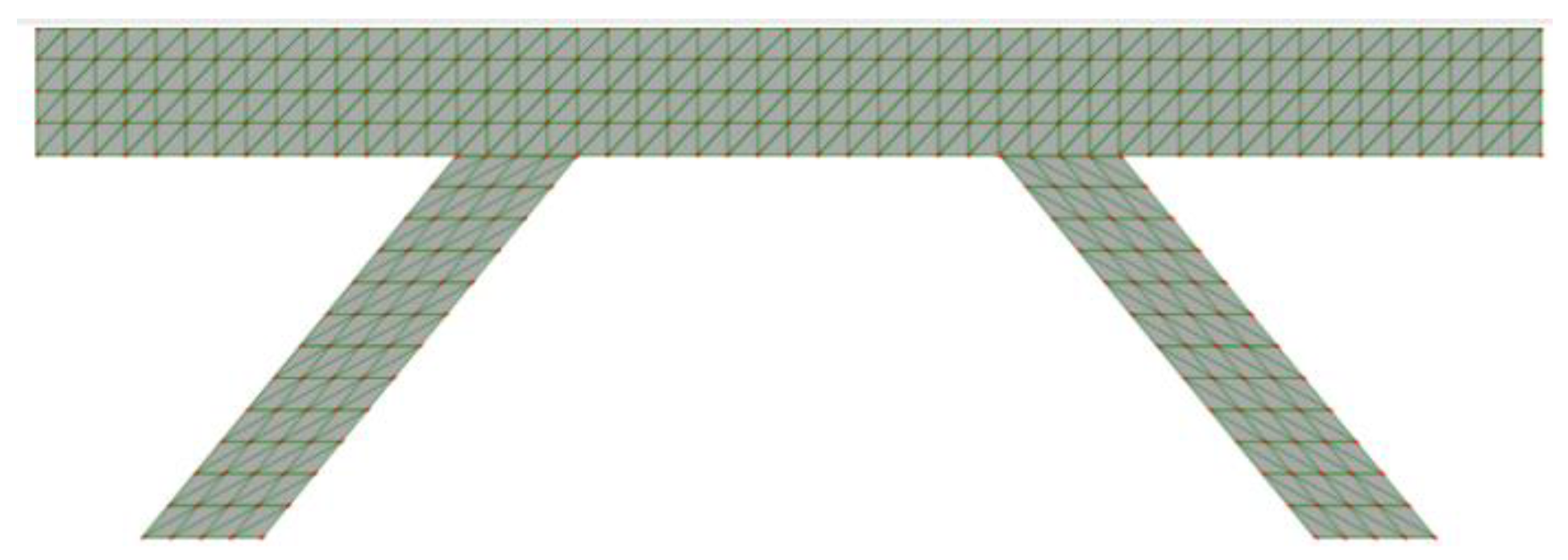
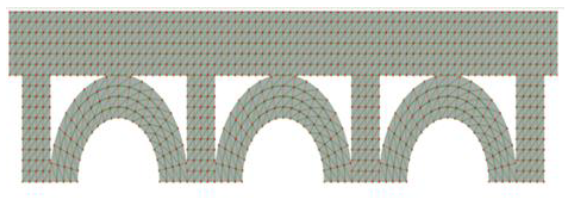
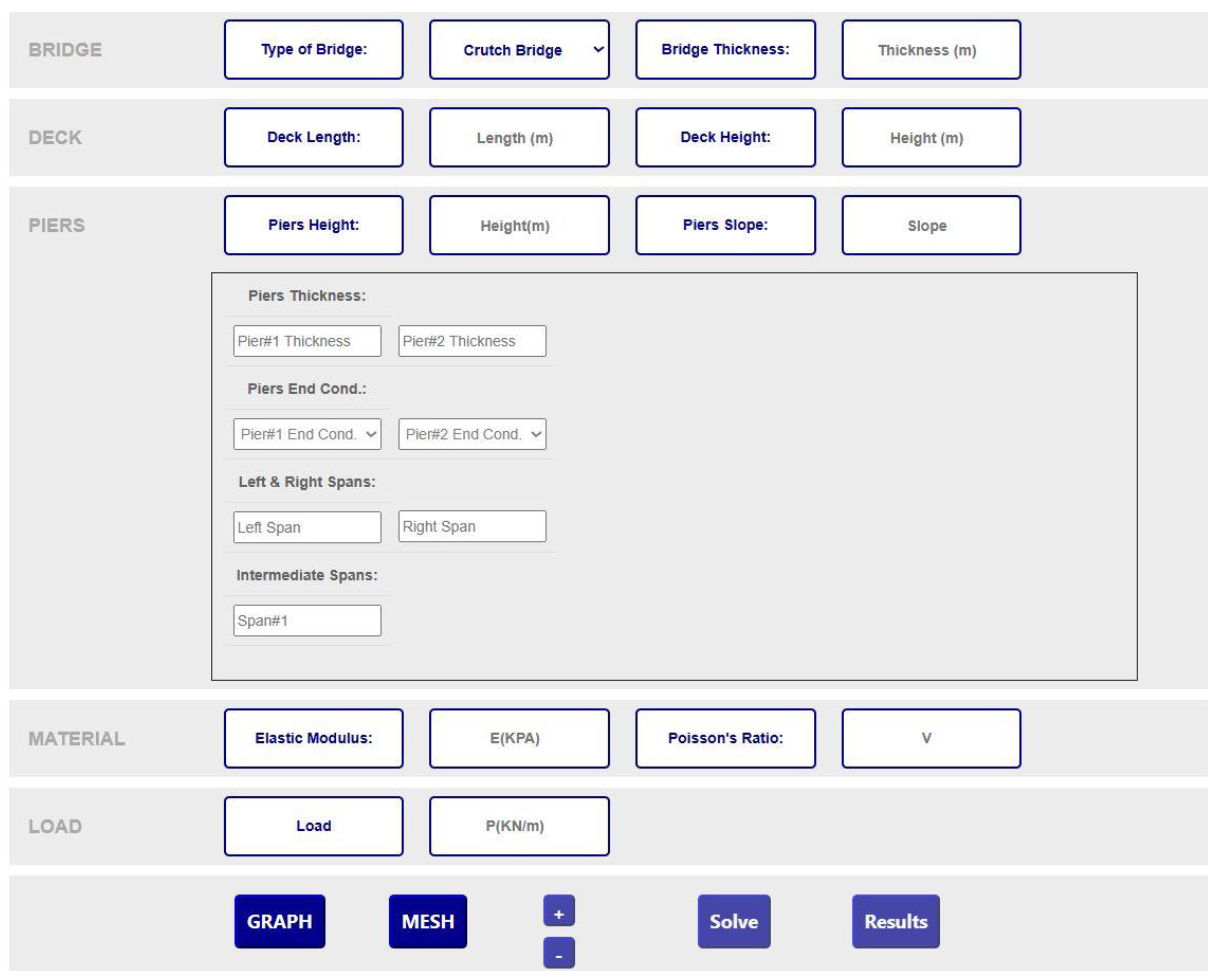
7. Case Study: Engineering Application for Finite Element Method

7.1. Concept

Finite element codes were traditionally developed in Fortran [65] and then in Fortran 90 [66]. During the last couple of decades, FEM developers started to use other languages. Some of them advocate using objects and C++ language in order to handle complexity in finite element software.

Zimmermann et al. [67] described the governing principles for object-oriented finite element programming before describing an implementation using SmallTalk [68] and C++ [69]. Also, a number of authors [70] have described object-oriented implementations of the finite element method using C++.

Moreover, Nikishkov [71] described the design of an object-oriented Java finite element code for the 2D and 3D analysis of elastic and elasto-plastic structural solids. The code was developed using Java 1.5 and utilized the Java3D API to allow for the visualization of the results. On the other hand, a User Interface was not developed and model specification was handled via an input text file which was read using a scanner.

However, smartphone applications for finite element analysis have received little attention until now despite some commercial endeavors, so there are very few studies concerning the development of a finite element code that takes into consideration the specifications and limitations of a smartphone. For example, a paper published by B.J Mac Donald [72], concerning a very simple finite element application that only solves 1D and 2D truss problems. Moreover, there are no studies concerning smartphone applications that solve large finite element problems, for complex structures.

One of the important reasons for this delay in FEA mobile application studies is the orientation of current developments towards cloud-based simulation instead of smartphone-based simulation. For example, MATLAB Mobile is MATLAB’s mobile application that connects the user to the MathWorks cloud where all operations and data are sent from the mobile to the MathWorks server to be processed [6]. Such development renders the smartphone a mere outlet of connection and not the base of operations.

Finally, with the increase in system demands by simulations and modeling, FEA smartphone applications stand currently behind in advancement and innovation compared to their PC counterpart.

7.2. Proposed Solution

The two main challenges here revolve around scientific calculations, both concerning memory costs and output precision. This is due to the number of the elements involved in each output generation as well as the scaling of element numbers.

7.2.1. Optimizing Memory Costs for Scientific Calculations

The approach for FEA smartphone application, taking into consideration the limitation of smartphones in terms of memory consumption, is, first, by the creation of a predefined mesh with a fast refinement procedure that is presented in this article. Moreover, in the next stage of work, the management of computational memory allocation is studied. The linear triangular element is chosen for meshing in the application. The linear triangular element is a two-dimensional finite element. This element can be used for the problems of plane stress or plane strain in elasticity. The linear triangular element has a modulus of elasticity E, a Poisson’s ratio ν, and a thickness t. Each linear triangle has three nodes with two degrees of freedom in the plane at each node, as shown in Figure 19. The global coordinates of the three nodes are denoted (Xi, Yi), (Xj, Yj), and (Xm, Ym). The order of nodes for each element is important—they should be listed counter-clockwise starting from any node.

The element stiffness matrix is given by [73]:

$$K^e=\det \left(J\right){{\displaystyle \int }}_{A_e}^{}d\xi d\eta =\frac{1}{2}\det \left(J\right)t{\left(B^e\right)}^{T}D{B}^e$$

where the three nodes matrix $B^e$ is:

$$B^e=\frac{1}{\det \left(J\right)}\left(\begin{array}{cccccc}{J}_{22}& 0& -J_{12}& 0& -J_{22}+J_{12}& 0\\ 0& -J_{21}& 0& J_{11}& 0& J_{21}-J_{11}\\ -J_{21}& J_{22}& J_{11}& -J_{12}& J_{21}-J_{11}& -J_{22}+J_{12}\end{array}\right)$$

And the Jacobien is:

$$J=\left(\begin{array}{cc}\frac{\partial x}{\partial \xi }& \frac{\partial y}{\partial \xi }\\ \frac{\partial x}{\partial \eta }& \frac{\partial y}{\partial \eta }\end{array}\right)=\left(\begin{array}{cc}{x}_1-x_3& y_1-y_3\\ x_2-x_3& y_2-y_3\end{array}\right)=\left(\begin{array}{cc}{J}_{11}& J_{12}\\ J_{21}& J_{22}\end{array}\right)$$

For cases of plane stress, the matrix [D] is given by

$$\left[D\right]=\frac{E}{\left(1+v\right)\left(1-2v\right)}\left[\begin{array}{ccc}1-v& v& 0\\ v& 1-v& 0\\ 0& 0& \frac{1-2v}{2}\end{array}\right]$$

For cases of plane strain, the matrix [D] is given by

$$\left[D\right]=\frac{E}{\left(1+v\right)\left(1-2v\right)}\left[\begin{array}{ccc}1-v& v& 0\\ v& 1-v& 0\\ 0& 0& \frac{1-2v}{2}\end{array}\right]$$

The global stiffness matrix is obtained through the assembly process. The algorithm for assembling the stiffness matrix consists of the following steps:

1. Initialize the global stiffness matrix K with zeros, sized (2n × 2n), where n is the total number of nodes in the system.

2. Iterate through each element in the mesh:

a. Determine the element stiffness matrix $K^e$ for the current element from the equation above.

b. Retrieve the global node indices associated with the element.

c. Add the local stiffness matrix ${\mathrm{K}}^{\mathrm{e}}$ to the corresponding submatrix of K using the global node indices.

3. Return the assembled global stiffness matrix K.

It is clear that the linear triangular element has six degrees of freedom, two at each node. Consequently, for a structure with n numbers of nodes, the global stiffness matrix K will be of size 2n × 2n (since we have two degrees of freedom at each node).

Once the global stiffness matrix K is obtained, the following structure equation is:

$$\left[K\right]\left[U\right]=\left[F\right]$$

(1)

where U is the global nodal displacement vector and F is the global nodal force vector. At this step, the boundary conditions are applied to the vectors U and F. Then, the matrix Equation (1) is solved.

In the finite element analysis conducted, force and displacement boundary conditions were incorporated to accurately simulate the behavior of the system. The force boundary condition was defined as:

F = F₀

where F represents the nodal force vector and F₀ is the prescribed force vector applied at specific nodes. The components of F₀ were determined based on the magnitude and direction of the applied forces, taking into account the physical requirements of the problem.

Simultaneously, the displacement boundary condition was expressed as:

U = U₀

where U represents the nodal displacement vector and U₀ denotes the prescribed displacement vector imposed at designated nodes.

Finally, once the unknown displacements and reactions are found from Equation (1), the stress and strain vectors are obtained for each element as follows:

$$\left[\epsilon \right]=\left[B\right]\left[u\right]$$

(2)

$$\left[\sigma \right]=\left[D\right]\left[\epsilon \right]$$

(3)

where [σ] is the stress vector in the element (of size 3 × 1) and [u] is the (6 × 1) element displacement vector. The vector a is written for each element as {σ} = $\left[{\sigma }_x {\sigma }_y {\tau }_{xy}\right]$.

The solution for the second part of the solution is explored in the same applications as well. It is to be noted that optimizing in scientific calculations is not only done in the main general algorithm but in the basic operations as well. In relation to this algorithm, one of the potentially largest memory cost operations is the matrix inverse, especially because of the large number of elements in each matrix. Adopting an iterative method of solving the matrix inverse instead of the direct method would significantly reduce memory costs. To further understand this, the two methods are presented.

Matrix inverse direct method:

$$A^{-1}=\frac{1}{\left|A\right|}\tilde{A}$$

$\mathrm{Equations} \mathrm{set} \mathrm{to} 10\times 10 \mathrm{determinant} \mathrm{calculation}\max \mathrm{per} \mathrm{equation}$

$$Iterations for \left|A\right|=n{\displaystyle \prod }_{i=1}^{n-10}{\left(n-i\right)}^{}$$

${\mathrm{Set} \mathrm{M}}_{\mathrm{ij}}{ \mathrm{submatrix} \mathrm{by} \mathrm{removing} \mathrm{i}}^{\mathrm{th}}{\mathrm{row} \mathrm{and} \mathrm{j}}^{\mathrm{th}}\mathrm{column} \mathrm{from} \mathrm{A}$

$$A_{ij}=\left|M_{ij}\right|$$

$$Iterations for \left|M_{ij}\right|=n^2{\displaystyle \prod }_{i=2}^{n-10}{\left(n-i\right)}^{}$$

$\mathrm{Total} \mathrm{major} \mathrm{iterations}: T=n{\displaystyle \prod }_{i=1}^{n-10}{\left(n-i\right)}^{}$ + $n^2{\displaystyle \prod }_{i=2}^{n-10}{\left(n-i\right)}^{}$.

The resultant space complexity for subjugate matrix calculation is represented as:

$$M=n^2\left(4+8\right)+4n^2{(n-1)}^2$$

Matrix inverse iterative method:

This method is based on the Gauss–Jordan matrix inversion. One of the strongest points of the method is the removal of the need to calculate the determinant.

The resultant space complexity is found as:

$$M=64n^2$$

The difference in the results between the two approaches highlights the cascading impact of altering even the smallest of operations on the entire performance and requirements of the simulation.

7.2.2. Challenge: Precision of Algorithms in Scientific Calculations

In order to present a more optimized graphical interface that reduces memory requirements, and takes into consideration the limitations of a smartphone in memory, a specific mesh is developed. This is a predefined mesh for a structure of defined geometry, these geometric shapes are actually suitable for shapes for bridges.

The approach presented consists of two steps: (1) an initial node placement is obtained using a linear node distribution, and (2) a fast refinement procedure is performed for 6-node triangular meshes or large-scale meshes in order to obtain an accurate solution and precision.

Therefore, a mesh is presented for three structural shapes: rectangular shape, trapezoidal, and arch shape.

First, for the rectangular-shaped structure, the “MeshGeneratorForRectangularShape” function is created. The “MeshGeneratorForRectangularShape” function generates a structured triangular mesh for a rectangular-shaped structure for finite element analysis.

As outputs, the code generates a 3-node triangular mesh and the coordinates x and y of each element node also we obtained the total number of elements and nodes.

The inputs are the following: dimensions of the rectangle in each direction (width and height) and the number of divisions in each direction x and y which depend on the level of mesh refinement requested.

For example:

L_x = width of the rectangular structure

L_y = height of the rectangular structure

N_x = number of divisions on the x-axis

N_y = number of divisions on the y-axis

The number of elements is:

$$N_E=\left(2N_X\right)\times N_Y.$$

And the number of nodes is:

$$N_N=\left(N_x+1\right)\times \left(N_Y+1\right).$$

So, for a girder bridge which is presented in the figure below, the bridge length is equal to 40 m, consisting of 4 piers with 2 m thick and 6 m high each.

As it is shown in Figure 20 below, the algorithm generates 240 elements and 144 nodes for the rectangular structure (girder 40 × 3 m) with respect to 40 divisions on the x-axis and 3 on the y-axis.

Also, in the mesh generator, a coarse mesh obtained is successively refined to produce a finer mesh. In addition, the refinement allows us to create a 6-node triangulation easily. A regular refinement is used; all triangles are divided into four triangles of the same shape by bisection of their edges.

So, by taking the example presented in Figure 20, the refinement of the grider mesh increases the number of elements from 240 to 960 (Figure 21a), then to 3840 elements (Figure 21b).

A triangular mesh for a trapezoidal-shaped structure is also developed by using the transformation matrix. The function “context.setTransform(a,b,c,d,e,f)” and a built-in function in Canvas.js allows us to easily transform a rectangular structure into a trapezoidal one. Figure 22 below shows the mesh of the trapezoidal-shaped part of the crutch bridge.

Similarly, a triangular mesh of arc-shaped structures is created, the nodes are spaced along the perimeter of the arc, and then it is offset by a distance that depends on the level of refinement. Figure 23 below shows the mesh of the arc-shaped part of the arch bridge.

7.3. Application

The finite element calculation consists of several steps that should be followed sequentially in order to reach the desired result.

Here are all the steps required:

• Step 1: Discretizing the domain—this step involves subdividing the domain into elements and nodes;
• Step 2: Writing the element stiffness matrix—the element stiffness equations need to be written for each element in the domain;
• Step 3: Assembling the global stiffness matrix—this will be done using the direct stiffness approach;
• Step 4: Applying the boundary conditions—like supports, applied loads and displacements;
• Step 5: Solving the linear equations [A] [X] = [B];
• Step 6: Post-processing—to obtain the reactions, element forces and stresses.

This application presents various types of bridges, three of these bridges are presented here: girder bridge, crutch bridge and arch bridge users can specify the dimensions of each part of the bridge, including the number of piers and arches, as well as choose the material specifications, the boundary conditions and input loads; see Figure 24. Here, Figure 25, Figure 26 and Figure 27 present the codes in JavaScript.

The application also generates the meshing process as seen in the previous section of this case study. The meshing is generated based on the previously discussed calculations.

Regarding the results, we are presenting below the yy-stress and y-deformation results for a concrete girder bridge supporting a linear load of 400 kN/m. The figures below show two sets of images for each result: the first set shows the result obtained from our application, while the second set shows the result obtained from the RDM6 software. We have validated the results obtained from our application by comparing them with the results obtained from the RDM6 software and found them to be consistent. Figure 28 and Figure 29 show the deformation and stress results.

8. Conclusions

This paper aimed to conceptualize and assess the challenges related to the development of engineering applications for the smartphone platform. The conducted state of the art shows that this concept is still in its early phase where the related applications are mostly an extension to smartphone tools or a connection to other servers and not independent simulation applications. While the reasons behind the lack of this type of application are not related to the domain of engineering, simulations in this field are considered heavy and demanding both in hardware/software. Nevertheless, the demand for it is evidently present which leads to this work. The challenges presented were explored in order to properly formulate and develop the basis of an achievable solution as seen previously. The presented solutions show that a change in the smartphone hardware/software is not sufficient to achieve the goal but a change in the culture of thought, and the basis of the developed algorithms is needed as well. The presented case studies show the development of applications that follow this new approach in the fields of control, composite materials, and the finite element method. These case studies show an effective approach to the challenges presented alongside a working solution. The goal of these solutions is mainly to optimize memory costs on several levels, whether it is on the front end (GUI) or the back end (algorithm execution), hence tackling the major cause behind the discussed challenges. The adoption of these solutions allows the bypassing of these challenges which in turn increases the potential and depth of future engineering applications on smartphones. This would allow further development and improvement of such types of applications where research in this field remains in its early stages. However, while the solutions given here are general approaches to a standard engineering application, the challenge related to memory cost and precision of algorithms differ between each engineering field because of the need for mathematical optimization of specific algorithms used. This mathematical optimization of standard algorithms in the concerned fields is the primary focus of future work because of the impact of this optimization on the general performance of the application and the relatively higher difficulty of achieving this solution.

References

1. International Data Corporation, Smartphone Shipments Declined in Fourth Quarter but 2021 Was Still a Growth Year with a 5.7% Increase in Shipments; IDC Media Center: Needham, MA, USA, 2022.
2. International Data Corporation, PC Demand Remained Strong in the Second Quarter Amid Early Signs That Market Conditions May Be Cooling, According to IDC; IDC Media Center: Needham, MA, USA, 2022.
3. Taylor, P. Global Smartphone unit shipments 2009–2022. In Statista Technology & Telecommunications; Statista: Hamburg, Germany, 2023. [Google Scholar]
4. GSMA. The Mobile Economy 2021; GSM Association: London, UK, 2021. [Google Scholar]
5. Zaher, M.; Greenwood, D.; Marzouk, M. Mobile Augmented Reality Applications for Construction Projects. Constr. Innov. 2018, 18, 152–166. [Google Scholar] [CrossRef]
6. Matlab. Matlab Documentation, Matlab Help; Matlab: Natick, MA, USA, 2022. [Google Scholar]
7. Phongtraychak, A.; Dolgaya, D. Evolution of Mobile Applications. MATEC Web Conf. 2018, 155, 01027. [Google Scholar] [CrossRef]
8. Hayfaa, M.; Subhi, Z.; Rizgar, Z.; Mohammed, S. A Comprehensive Study of Kernel (Issues and Concepts) in different operating systems. Asian J. Res. Comput. Sci. Inf. Technol. 2021, 8, 16–31. [Google Scholar]
9. Department of Computer Science and Engineering. School of Computing, Mobile Application Development, Sathyabama, Institute of Science and Technology. Available online: https://www.sathyabama.ac.in/course-materials/mobile-application-development-0 (accessed on 4 March 2023).
10. SCarvalho; Aniche, M.; Verssimo, J.; Durelli, R.; Gerosa, M. An empirical catalog of code smells for the presentation layer of Android apps. Empir. Softw. Eng. 2019, 24, 3546–3586. [Google Scholar] [CrossRef]
11. Vishal, K.; Kushwaha, S. Mobile Application Development Research Based on Xamarin Platform. In Proceedings of the 4th International Conference on Computing Sciences (ICCS), Jalandhar, India, 30–31 August 2018; pp. 115–118. [Google Scholar]
12. Swetina, J.; Lu, G.; Jacobs, P.; Ennesser, F.; Song, J. Toward a standardized common M2M service layer platform: Introduction to oneM2M. IEEE Wirel. Commun. 2014, 21, 20–26. [Google Scholar] [CrossRef]
13. Qian, F.; Wang, Z.; Gerber, A.; Mao, Z.; Sen, S.; Spatscheck, O. Profiling resource usage for mobile applications: A cross-layer approach. In Proceedings of the 9th International Conference on Mobile Systems, Applications, and Services, Bethesda, MD, USA, 28 June 2011–1 July 2011; pp. 321–334. [Google Scholar]
14. Chau, N.; Jung, S. Dynamic analysis with Android conatiner: Challenges and opportunities. Digit. Investig. 2018, 27, 38–46. [Google Scholar] [CrossRef]
15. Welderufael, T.; Aleksy, M.; Andersson, K.; Lehtola, M. Mobile Computing Application for Industrial Field Service Engineering: A Case for ABB Service Engineers. In Proceedings of the 38th Annual IEEE Conference on Local Computer Networks, Sydney, NSW, Australia, 21–24 October 2013; pp. 188–193. [Google Scholar]
16. Moustefaoui, G.; Tariq, F. Mobile Apps Engineering: Design, Development, Security, and Testing; CRC Press: Boca Raton, FL, USA, 2018. [Google Scholar]
17. Pei-Huang, D.; Naai-Jung, S. BIM-Based AR Maintenance System (BARMS) as an Intelligent Instruction Platform for Complex Plumbing Facilities. Appl. Sci. 2019, 9, 1592. [Google Scholar]
18. Williams, G.; Gheisari, M.; Chen, P. An efficient BIM Translation to Mobile augmented reality applications. J. Manag. Eng. 2015, 31, A4014009. [Google Scholar] [CrossRef]
19. VisualLive, Mobilive, Mixed Reality (AR) for iOS/Android, VisualLive. Available online: https://visuallive.nl/mobilive-mixed-reality-ar-for-ios-android/ (accessed on 5 March 2023).
20. Meza, S.; Turk, Z.; Dolenc, M. Measuring the potential of augmented reality in civil engineering. Adv. Eng. Softw. 2015, 90, 1–10. [Google Scholar] [CrossRef]
21. Golpavar, F. Assessment of Collaborative Decision-Making in Design Development. Master’s Thesis, University of British Columbia, Vancouver, BC, Canada, 2006. [Google Scholar]
22. Shakil, A. A Review on Using Opportunities of Augmented Reality and Virtual Reality in Construction Project Management. OTMC Int. J. 2019, 10, 1839–1852. [Google Scholar]
23. Yoora, P.; Hyojoo, S.; Changwan, K. Investigating the determinants of construction professionals’ acceptance of web-based training: An extension of the technology acceptance model. Autom. Constr. 2012, 22, 377–386. [Google Scholar]
24. Nazar, A.; Jiao, P.; Zhang, Q.; Egbe, K.; Alavi, A. A new structural health monitoring approach based on smartphone measurements of magnetic field intensity. IEEE Instrum. Meas. Mag. 2021, 24, 49–58. [Google Scholar] [CrossRef]
25. Park, D.H.; Heo, J.M.; Jeong, W.; Yoo, Y.H.; Park, B.J. Smartphone-Based VOC Sensor Using Colorimetric Polydiacetylenes. ACS Appl. Mater. Interfaces 2018, 10, 5014–5021. [Google Scholar] [CrossRef]
26. Minichiello, A.; Armijo, D.; Mukherjee, S.; Caldwell, L.; Kulyukin, V.; Truscott, T.; Elliott, J.; Bhouraskar, A. Developing a mobile application-based particle image velocimetry tool for enhanced teaching and learning in fluid mechanics: A design-based research approach. Comput. Appl. Eng. Educ. 2020, 29, 517–537. [Google Scholar] [CrossRef]
27. De Oliveira, M.T.; Maija, M.; Leslie, M.; Terhi, L.; Sarang, T.; Ville, L. Towards tropospheric delay estimation using GNSS smartphone receiver network. Adv. Space Res. 2021, 68, 4794–4805. [Google Scholar] [CrossRef]
28. Kanetaki, Z.; Stergiou, C.; Bekas, G.; Kanetaki, E. Machine Learning and Statistical Analysis applied on Mechanical Engineering CAD course: A Case Study During ERTE Pahse in the Context of Higher Education. In Proceedings of the 2020 4th International Symposium on Multidisciplinary Studies and Innovative Technologies, Istanbul, Turkey, 22–24 October 2020. [Google Scholar]
29. Modic, E. Linear Bearing CAD Models on the Fly; Today’s Medical Development: Valley View, OH, USA, 2018. [Google Scholar]
30. Olivotti, D.; Dreyer, S.; Kolsch, P.; Herder, C.; Breitner, M.; Aurich, J. Realizing availability-oriented business models in the capital goods industry. In Proceedings of the 10th CIRP Conference on Industrial Product-Service Systems, IPS2 2018, Linköping, Sweden, 29–31 May 2018; pp. 29–31. [Google Scholar]
31. Kahriman, F.; Liland, K. SelectWave: A graphical user interface for wavelength selection and spectral data analysis. Chenometrics Intell. Lab. Syst. 2021, 212, 104275. [Google Scholar] [CrossRef]
32. Zanfardimo, M.; Castaldo, R. MuSA: A graphical user interface for multi-OMICs data integration in radiogenomic studies. Sci. Rep. 2021, 11, 1550. [Google Scholar] [CrossRef]
33. Carruth, D.; Hudson, C.; Fox, A.; Deb, S. User Interface for an Immersive Virtual Reality Greenhouse for Training Precision Agriculture. In HCII 2020: Virtual, Augmented and Mixed Reality. Industrial and Everyday Life Applications; Springer International Publishing: Berlin/Heidelberg, Germany, 2020. [Google Scholar]
34. Alturki, R.; Gay, V. Usability Attributes for Mobile Applications, a Systematic review; Faculty of Engineering and Information Technology, University of Technology Sidney: Ultimo, NSW, Australia, 2018. [Google Scholar]
35. Punchoojit, L. Usability Studies on Mobile User Interface Design Patterns: A Systematic Literature Review. Adv. Hum.-Comput. Interact. 2017, 2017, 6787504. [Google Scholar] [CrossRef]
36. Bennett, K.; Nagy, A.; Flash, J. Visual Display, Handbook of Human Factors and Ergonomics; John Wiley & Sons: Hoboken, NJ, USA, 2012. [Google Scholar]
37. Abdalha, A.; Muasaad, A. A study of the interface usability issues of mobile learning applications for smartphones from the user’s perspective. In Proceedings of the International Journal on Integrating Technology in Education (IJITE), Lyon, France, 19–22 May 2008; Volume 3. [Google Scholar]
38. Deelman, E.; Chervenak, A. Data Management Challenges of Data-Intensive Scientific Workflows. In Proceedings of the 2008 Eighth IEEE International Symposium on Cluster Computing and the Grid, Lyon, France, 19–22 May 2008. [Google Scholar]
39. Sosa, J.; Thomas, P.; Delia, L.; Caseres, J. Mobile Application Development Approaches: A Comparative Analysis on the Use of Storage Space. In Argentine Congress of Computer Science XXIV; SEDICI: Seaford, UK, 2018. [Google Scholar]
40. Vandenbrouke, K.; Ferreira, D.; Goncalvez, J. Mobile cloud storage: A contextual experience. In Proceedings of the 16th International Conference on Human-Computer Interaction with Mobile Devices & Services, Toronto, ON, Canada, 23–26 September 2014. [Google Scholar]
41. Li, C.; Bai, J.; Tang, J. Joint optimization of data placement and scheduling for improving user experience in edge computing. J. Parallel Distrib. Comput. 2019, 125, 93–105. [Google Scholar] [CrossRef]
42. Carroll, A.; Heiser, G. An Analysis of Power Consumption in a Smartphone. In Proceedings of the 2010 USENIX Conference on USENIX Annual Technical Conference, Boston, MA, USA, 22–25 June 2010. [Google Scholar]
43. Ataeeshojai, M.; Elliott, R.; Krzymien, W.; Tellambura, C.; Maljevic, I. Iterative Matrix Inversion Methods for Precoding in Cell-Free Massive MIMO Systems. IEEE Trans. Veh. Technol. 2022, 71, 11972–11987. [Google Scholar] [CrossRef]
44. Albreem, M. Approximate Matrix Inversion Methods for Massive MIMO Detectors. In Proceedings of the IEEE 23rd International Symposium on Consumer Technologies (ISCT), Ancona, Italy, 19–21 June 2019. [Google Scholar]
45. Wu, J.; Bose, A. A new successive relaxation scheme for the W-matrix solution method on a shared memory parallel computer. IEEE Trans. Power Syst. 1996, 11, 233–238. [Google Scholar]
46. Williamson, D.; Shmoys, D. The Design of Approximation Algorithms; Cambridge University Press: Cambridge, UK, 2011. [Google Scholar]
47. Hanrahan, G.; Patil, D. Chemometrics & Statistics; Multivariate Calibration Techniques, Encyclopedia of Analytical Science, 7th ed.; Elsevier: Amsterdam, The Netherlands, 2005. [Google Scholar]
48. Steinwart, I.; Hush, D.; Scovel, C. Optimal Rates for Regularized Least Squares Regression; Los Alamos National Laboratory: Los Alamos, NM, USA, 2009. [Google Scholar]
49. Cooper, K.; Harvey, T. Compiler-controlled memory. ACM SIGOPS Oper. Syst. Rev. 1998, 32, 2–11. [Google Scholar] [CrossRef]
50. Ou, P.; Desmky, B. Towards understanding the costs of avoiding out-of-thin-air results. In Proceedings of the ACM on Programming Languages, Boston, MA, USA, 24 October 2018; Volume 2. [Google Scholar]
51. Gotz, S.; Tichy, M.; Kehrer, T. Dedicated Model Transformation Languages vs. General-Purpose Languages: A Historical Perspective on ATL vs. Java; Science & Technology Publications: Setúbal, Portugal, 2021. [Google Scholar]
52. Hopner, S.; Kehrer, T.; Tichy, M. Contrasting dedicated model transformation languages versus general purpose languages: A historical perspective on ATL versus Java based on complexity and size. Softw. Syst. Model. 2022, 21, 805–837. [Google Scholar] [CrossRef]
53. Gotz, S.; Tichy, M.; Kehrer, T. Claimed advantages and disadvantages of (dedicated) model transformation languages: A systematic literature review. Softw. Syst. Model. 2021, 20, 469–503. [Google Scholar] [CrossRef]
54. Van Den Brouke, B.; Tumer, F.; Lomov, S.; Verpoest, I.; De Luka, P.; Dufort, L. Micro–macro structural analysis of textile composite parts: Case study. In Proceedings of the 25th International SAMPE Europe Conference, Paris, France, 30 March–1 April 2004. [Google Scholar]
55. Lomov, S.; Van Den Brouke, B.; Tumer, F.; Verpoest, I.; De Luka, P.; Dufort, L. Micro–macro structural analysis of textile composite parts. In Proceedings of the ECCM-11, Rodos, Greece, 31 May–3 June 2004; pp. 194–199. [Google Scholar]
56. Gommers, B.; Verpoest, I.; Van Houtte, P. The Mori–Tanaka method applied to textile composite materials. Acta Mater. 1998, 46, 2223–2235. [Google Scholar] [CrossRef]
57. Lomov, S.; Truevtzev, N. A software package for the prediction of woven fabrics geometrical and mechanical properties. Fibres Text East Eur. 1995, 3, 49–52. [Google Scholar]
58. Belov, E.; Lomov, S.; Verpoest, I.; Peeters, T.; Roose, D.; Parnas, R. Modelling of permeability of textile reinforcements: Modelling of permeability of textile reinforcements. Compos. Sci. Tecnol. 2004. [Google Scholar] [CrossRef]
59. Carvelli, V.; Chi, T.; Larosa, M.; Lomov, S.; Poggi, C.; Ranz, D. Experimental and numerical determination of the mechanical properties of multi-axial multiply composites. In Proceedings of the ECCM-11, Rodos, Greece, 31 May–3 June 2004. [Google Scholar]
60. Lomov, S.; Mikolanda, T. Textile Virtual Reality. In Proceedings of the TechTextile Symposium, Frankfurt, Germany, 6–9 June 2005. [Google Scholar]
61. Verspoest, I.; Lomov, S. Virtual Textile Composites Software: Integration with micromechanical, permeability and structural analysis. Compos. Sci. Technol. 2005, 65, 2563–2574. [Google Scholar] [CrossRef]
62. ASTM. A Standard Test Method for Tensile Properties of Polymer Matrix Composite Materials; ASTM: West Conshohocken, PA, USA, 2008. [Google Scholar]
63. Blacklock, M.; Shaw, J.; Zok, F.; Cox, B. Virtual Specimens for analyzing strain distributions in textile ceramic composite. Compos. Part A Appl. Sci. Manuf. 2016, 85, 40–51. [Google Scholar] [CrossRef]
64. Kaddaha, M.; Younes, R.; Lafon, P. New Geometrical Modelling for 2D Fabric and 2.5D Interlock Composites. Textiles 2022, 2, 142–161. [Google Scholar] [CrossRef]
65. Bathe, K. Finite Element Procedures; Prentice-Hall: Englewood Cliffs, NJ, USA, 1996. [Google Scholar]
66. Smith, I.; Griffiths, D. Programming the Finite Element Method; Wiley: Chichester, UK, 1998. [Google Scholar]
67. Zimmerman, T.; Dubois, Y.; Bomme, P. Object-oriented Finite Element Programming: I. Governing Principles. Comput. Methods Appl. Mech. Eng. 1992, 98, 291–303. [Google Scholar] [CrossRef]
68. Zimmerman, T.; Dubois, Y.; Bomme, P. Object-oriented Finite Element Programming: II. A Prototype Program in Smalltalk. Comput. Methods Appl. Mech. Eng. 1992, 98, 361–397. [Google Scholar] [CrossRef]
69. Zimmerman, T.; Dubois, Y.; Bomme, P. Object-oriented Finite Element Programming: II. An Efficient Implementation in C++. Comput. Methods Appl. Mech. Eng. 1993, 108, 165–183. [Google Scholar]
70. Donescu, P.; Laursen, T. A Generalized Object-Oriented Approach to Solving Ordinary and Partial Differential Equations Using Finite Elements. Finite Elements Anal. Des. 1996, 22, 93–107. [Google Scholar] [CrossRef]
71. Nikishkov, G. Object Oriented Design of a Finite Element Code in Java. Comput. Model. Eng. Sci. 2006, 11, 81–90. [Google Scholar]
72. Macdonald, B. An Object-Oriented Smarpthone Application for Structural Finite Element Analysis. Int. J. Adv. Comput. Sci. Appl. 2014, 5, 59–66. [Google Scholar]
73. Calcul Des Structures Par Elements Finis Legay PDF. Available online: http://antoinelegay.free.fr/Calcul_des_structures_par_elements_finis_Legay.pdf (accessed on 20 April 2023).
Figure 1. Smartphone and desktop sales (in millions). This figure was adapted from [3].
Software 02 00017 g001
Figure 2. Mobile application architecture. This figure was adapted from [9].
Software 02 00017 g002
Figure 3. VisualLive smartphone application [18].
Software 02 00017 g003
Figure 4. Medical CAD application [28].
Software 02 00017 g004
Figure 5. Smartphone scientific application challenges.
Software 02 00017 g005
Figure 6. Conventional interface and proposed interface for GUI.
Software 02 00017 g006
Figure 7. Tasks 1 and 2: memory cost pre-execution and after execution.
Software 02 00017 g007
Figure 8. Engineering application for systems control UX map.
Software 02 00017 g008
Figure 9. Model identification.
Software 02 00017 g009
Figure 10. Control scheme design choices.
Software 02 00017 g010
Figure 11. Toolbox prototype.
Software 02 00017 g011
Figure 12. Control simulation result.
Software 02 00017 g012
Figure 13. TexGen download storage.
Software 02 00017 g013
Figure 14. Saved example for 2.5 D interlock.
Software 02 00017 g014
Figure 15. Engineering application for composite material customization map.
Software 02 00017 g015
Figure 16. Plain weave and twill weave fabric.
Software 02 00017 g016
Figure 17. Sateen/satin weave fabric.
Software 02 00017 g017
Figure 18. Layer to layer.
Software 02 00017 g018
Figure 19. Linear triangular element.
Software 02 00017 g019
Figure 20. Grider bridge mesh.
Software 02 00017 g020
Figure 21. (a) Refined grider bridge mesh. (b) Refined grider bridge mesh.
Software 02 00017 g021
Figure 22. Crutch bridge mesh.
Software 02 00017 g022
Figure 23. Arch bridge mesh.
Software 02 00017 g023
Figure 24. Inputs options for a crutch bridge.
Software 02 00017 g024
Figure 25. Girder bridge.
Software 02 00017 g025
Figure 26. Crutch bridge.
Software 02 00017 g026
Figure 27. Arch bridge.
Software 02 00017 g027
Figure 28. y-deformation result.
Software 02 00017 g028
Figure 29. yy-stress result.
Software 02 00017 g029
Disclaimer/Publisher’s Note: The statements, opinions and data contained in all publications are solely those of the individual author(s) and contributor(s) and not of MDPI and/or the editor(s). MDPI and/or the editor(s) disclaim responsibility for any injury to people or property resulting from any ideas, methods, instructions or products referred to in the content.