Article

Comparing Measured Agile Software Development Metrics Using an Agile Model-Based Software Engineering Approach versus Scrum Only

Department of Systems Engineering, Walter Scott, Jr. College of Engineering, Colorado State University, Fort Collins, CO 80523, USA
*
Author to whom correspondence should be addressed.
Software 2023, 2(3), 310-331; https://doi.org/10.3390/software2030015
Submission received: 27 June 2023 / Revised: 18 July 2023 / Accepted: 20 July 2023 / Published: 26 July 2023
(This article belongs to the Topic Software Engineering and Applications)

Abstract

:
This study compares the reliability of estimation, productivity, and defect rate metrics for sprints driven by a specific instance of the agile approach (i.e., scrum) and an agile model-Bbased software engineering (MBSE) approach called the integrated Scrum Model-Based System Architecture Process (sMBSAP) when developing a software system. The quasi-experimental study conducted ten sprints using each approach. The approaches were then evaluated based on their effectiveness in helping the product development team estimate the backlog items that they could build during a time-boxed sprint and deliver more product backlog items (PBI) with fewer defects. The commitment reliability ( C R ) was calculated to compare the reliability of estimation with a measured average scrum-driven value of 0.81 versus a statistically different average sMBSAP-driven value of 0.94. Similarly, the average sprint velocity ( S V ) for the scrum-driven sprints was 26.8 versus 31.8 for the MBSAP-driven sprints. The average defect density ( D D ) for the scrum-driven sprints was 0.91, while that of the sMBSAP-driven sprints was 0.63. The average defect leakage ( D L ) for the scrum-driven sprints was 0.20, while that of the sMBSAP-driven sprints was 0.15. The t-test analysis concluded that the sMBSAP-driven sprints were associated with a statistically significant larger mean C R , S V , D D , and D L than that of the scrum-driven sprints. The overall results demonstrate formal quantitative benefits of an agile MBSE approach compared to an agile alone, thereby strengthening the case for considering agile MBSE methods within the software development community. Future work might include comparing agile and agile MBSE methods using alternative research designs and further software development objectives, techniques, and metrics.

1. Introduction

The increasing complexity of software systems makes the risk of failure higher [1]. Unfortunately, software projects often do fail [2]. Several works of the literature discuss the history, factors, and impact on information technology (IT) projects’ failure [3,4,5]. A study of 5400 large IT projects exceeding $15 million found that, on average, large IT projects run 45% over budget and 7% behind schedule while delivering 56% less value than initially planned [6]. Other work has found that software projects carry the highest risk of cost and schedule overruns [7]. The reasons for large IT project failures has been summarized into four categories: missing focus, content issues, skills issues, and execution issues. Examples of multi-million challenged information systems include the UK National Programme for IT (£10.1bn), the US Air Force Expeditionary Combat Support System ($1bn), FiReControl (£469m), MyCalPays ($373m), and others [8].
During the 1990s, a number of lightweight software development methods evolved in response to the prevailing heavyweight methods that were perceived as overly regulated and planned. These lightweight methods included: the Rapid Application Development (RAD), in 1991 [9]; the Agile Unified Process (AUP) [10], and the Dynamic Systems Development Method (DSDM) [11]—both conducted in 1994—the Scrum [12] in 1995; the Crystal Clear Method [13] and the Extreme Programming (XP) [14]—both conducted in 1996—and the Feature-Driven Development (FDD) [15] in 1997. These software methods are collectively referred to as agile software development methods, although these all originated before the publication of the Agile Manifesto.
One of the benefits of agile is its alignment with systems engineering models such as the ISO/IEC/IEEE 15288 standards [16] and the widely-used V-model [17]. As software systems increase in size and complexity, new approaches to abstraction, concurrency, and uncertainty must be devised [11]. Agile methodologies do provide realistic and appealing strategies to evolve systems and software engineering to address these concerns [11].
To help address the various challenges of software development, a Model-Based Software Engineering (MBSE) approach can support the management of information system complexity during the architecting and development process [18]. Some researchers have proposed combining MBSE with agile to leverage the benefits of both worlds in addressing the complexity of information technology systems, especially if adopted during the system architecting process [19,20,21,22,23,24]. However, sources that provide considerable and persuasive data about the convergence of MBSE and agile are still in their infancy, despite researchers’ efforts. The lack of research that quantitatively compares agile MBSE with agile one impedes the consideration of agile MBSE for technology-based systems.
This article aims to compare an instance of agile MBSE, called the Scrum Model-Based Systems Architecture Process (sMBSAP) [24], with scrum. sMBSAP integrates a particular MBSE approach, MBSAP [25], with a specific agile approach, scrum [26]. The overarching objective is to investigate how the software development performance using agile MBSE is compared to that of the agile methodology alone when developing software systems. This article specifically compares the reliability of estimation, productivity, and defect rate of the sMBSAP vs. that of scrum. This will be achieved by analyzing the results from a quasi-experimental study conducted to investigate the effects of sMBSAP and scrum on the software development performance while developing a software system for a health technology system.
The remainder of the paper is organized as follows. Section 2 provides a background of agile and agile MBSE methods, including the three dependent variables used in the experiment—reliability of estimation, productivity, and defect rate—and concludes with the research purpose. Section 3 explains the experimental design, techniques, and procedures used, and, finally, the factors are considered to minimize threats to reliability and validity. Section 4 presents the results of the experiment. Section 5 provides a conclusion and outlines future work that will be required to further explore the effect of agile MBSE on software development objectives.

2. Background

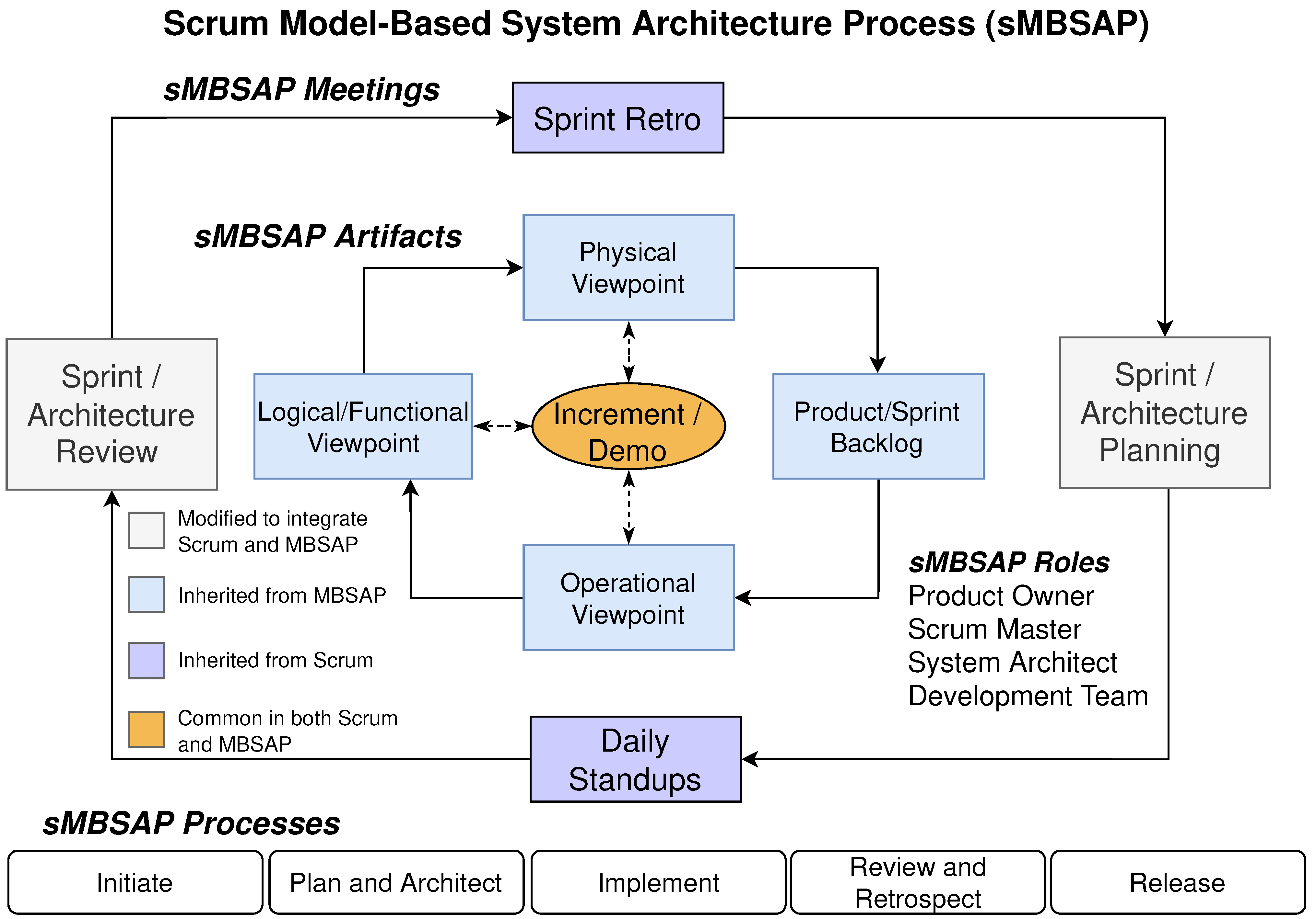
2.1. Scrum and Agile MBSE Methods

The scrum software development process is an agile method that is used for managing and directing the development of complex software and products by using incremental and iterative techniques [27]. Model-Based Software Engineering (MBSE) is a software development approach in which models play an important central role [28]. MBSE was developed to overcome the drawbacks of the conventional Document-Based Systems Engineering (DBSE) method, which became apparent as information-intensive systems became more complex [29]. The MBSAP outlines object-oriented design methods to create an architecture for a system through structured decomposition into modular and manageable levels of complexity by using object-oriented principles, such as abstraction, encapsulation, modularity, generalization, aggregation, interface definition, and polymorphism [25]. Agile MBSE presented itself as a possible solution for two issues that faced system development, namely, rigidity and waterfall orientation [11]. Agile MBSE also presented itself as a potential solution for the competing views and challenges related to documentation and requirement traceability [13,19].
Recent work by Huss et al. has developed an agile MBSE named sMBSAP, which involves a development method that integrates scrum and the MBSAP [24]. In addition to the main characteristics of scrum and the MBSAP, the sMBSAP emphasizes the engagement of the product development team in customizing the MBSE tool, using UML-based and non-UML-based models to describe the system and leveraging the built-in models (provided in some tools) to arrive at an initial version of the model more quickly. Figure 1 summarizes the sMBSAP meetings, artifacts, processes, and roles. The sMBSAP approach includes five main artifacts: product/sprint backlog, operational viewpoint (OV), logical/functional viewpoint (LV), physical viewpoint (PV), and product increment, as well as four roles: the product owner, scrum master, system architect, and product development team. The sMBSAP updates the artifacts to keep system information within the model. The five sMBSAP phases include initiate, plan and architect, implement, review and retrospect, and release. sMBSAP is application agnostic, as it can be applied to other software or engineered systems.

2.2. Reliability of Estimation

Effort estimation is a vital part of managing software projects. There is plenty of research regarding effort estimation models, techniques, and tools [30,31,32,33]. What makes estimation in agile software projects unique is that the software is developed incrementally, and customer feedback significantly influences the subsequent iterations. This also implies that product estimations and planning need to be done progressively. This is achieved in scrum by planning iteratively at three levels (i.e., release planning, sprint planning, and daily planning) [34]. Common estimation techniques in agile software development include expert opinion, analogy, and dis-aggregation [34]. Planning poker [35] is another widely used technique, especially in scrum [36,37]. A study about using planning poker for user story estimation found that planning poker produced more accurate estimates than unstructured group estimates [38]. Other studies found that planning poker in scrum projects yielded less optimistic and more accurate estimates than a statistical combination of individual expert estimates [39,40].
Estimation accuracy in software development has also been investigated. An in-depth study on 18 different companies and project managers of 52 different projects found that average effort overruns were 41%, and that the estimation performance has not changed much in the last 10–20 years [41]. Several researchers studied and analyzed the use of the commitment reliability ( C R ) metric (referred to as say/do ratio, estimation accuracy, or simply planned vs. actuals) in software projects [42,43,44,45]. Although agile teams use other reliability of estimation metrics, C R is the most widely used metric in practice. The C R metric used by agile teams is identical to the earned value (EV) metric, which is part of the earned value management (EVM) methodology used in traditional project management.

2.3. Productivity

One of the reasons that scrum is widely used in agile software development is the positive correlation between scrum and project productivity [14]. Other outcomes such as product quality, client satisfaction, cost reduction, and team motivation have been found to be associated with productivity [14]. In a systematic review of productivity factors in software development, it was found that soft factors are often not analyzed with equal detail as more technical factors [46]. It has been argued that the factors influencing productivity depend on the business domain the software is produced for [47]. It has also been found that more than a third of the time a typical software developer spends is not concerned with technical work [48] and that reusability has a significant effect on productivity [49].
In software development, the count of lines of code ( C L O C ) and story points ( S P ) (sometimes referred to as function points) are traditionally used as measures of productivity [46]. sprint velocity ( S V ) is the number of S P completed by the product development team in one sprint [34]. Several researchers have studied and analyzed the use of S V in software projects [50,51,52]. Although agile teams use other metrics, the most influential metrics in many of the studies are S V and effort estimate [53]. S V is a function of the direction and speed [54]. Although the direction is more easily overlooked, both factors should be equally considered [54]. The challenge for teams is to decide how time should be split between ceremonies and product build tasks, have been investigated by researchers [55]. velocity fluctuation ( V F ) is a vital graph that product managers watch during sprint planning and execution because it helps them plan more accurately for future sprints. V F has been studied to identify the sources of issues arising in scrum implementations, and it was found that fluctuations in velocity are caused by the team missing their commitments that, in turn, depend on the unaccounted complexities of different sub-systems [56].

2.4. Defect Rate

IEEE defines error, defect, and failure in its standard glossary of software engineering terminology [57]. A software defect is an error in coding that causes failure in the software [58]. It is a form of deficiency that causes the software to produce an incorrect, unintended, or unexpected result [59]. An error is an incorrect action on the part of a programmer [57]. With software’s growing size and complexity, software testing plays a critical role in capturing software defects. Detecting and fixing software defects are the most expensive part of the software development lifecycle [60]. Researchers investigated the increasing cost of detecting defects throughout the software development lifecycle [61]. During the development step, detecting and fixing defects tend to cost $977 per defect; the cost increases to $7,136 (or 630%) per defect in the testing phase; then, it is further doubled in the maintenance phase, reaching $14,102 [62]. It is no wonder that software defect prediction is a popular research topic in the software development field with such high penalties [63].
Defect density ( D D ) is another widely used defect rate metric [64,65,66], which is defined as the number of defects divided by size [66]. Some researchers studied and calculated D D using thousands (Kilo) of lines of code ( K L O C ) as a measure of size [66]. Other researchers use other size metrics such as S P [67], user stories, or product backlog items (PBIs) [34,68], and developer’s efforts (measured by person-hours or man-days) [69]. The defect leakage ( D L ) [70,71,72,73] is another known defect rate metric, which is the ratio of defects found during testing vs. the defects found during the next phase.

2.5. Research Purpose

Although few researchers discuss the integration between MBSE and agile and their qualitative benefits, the literature that provides quantitative comparative analysis is still limited. This scarcity hinders considering agile MBSE as an option for technology-based systems. The literature sparsity on this problem leads to the following research question:
Comparing sMBSAP and scrum, are there measurable benefits to software development performance when using one approach over the other?
The return-on-investment (ROI) for software system development methodologies, including agile and MBSE, is commonly measured in terms of development cost, development time, impact on quality (measured in the number of defects) [74], accuracy in estimation, and increased productivity [75]. The purpose of this research is to conduct an experiment to compare the sMBSAP [24] and scrum in terms of the reliability of estimation, productivity, and defect rate. The development of a health tech system that provides dietary recommendations to users based on their health profile [24] was used as a context for this experiment.
In this experiment, the dependent variables were the software development performance, namely (1) the reliability of estimation; (2) the defect rate; and (3) the productivity. The categorical independent variable was the system development approach consisting of two groups: one treatment (sMBSAP) and one control (Scrum).

3. Research Methods

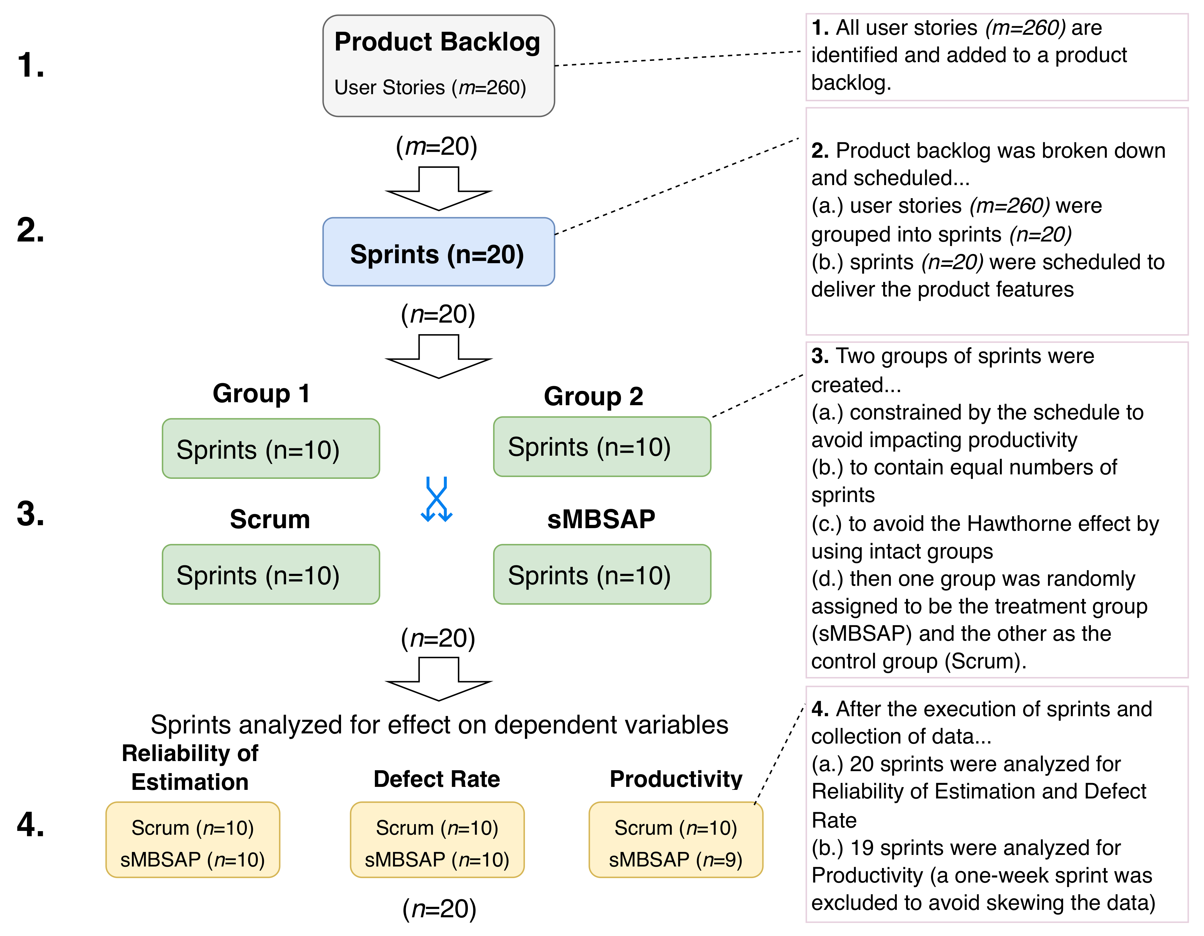
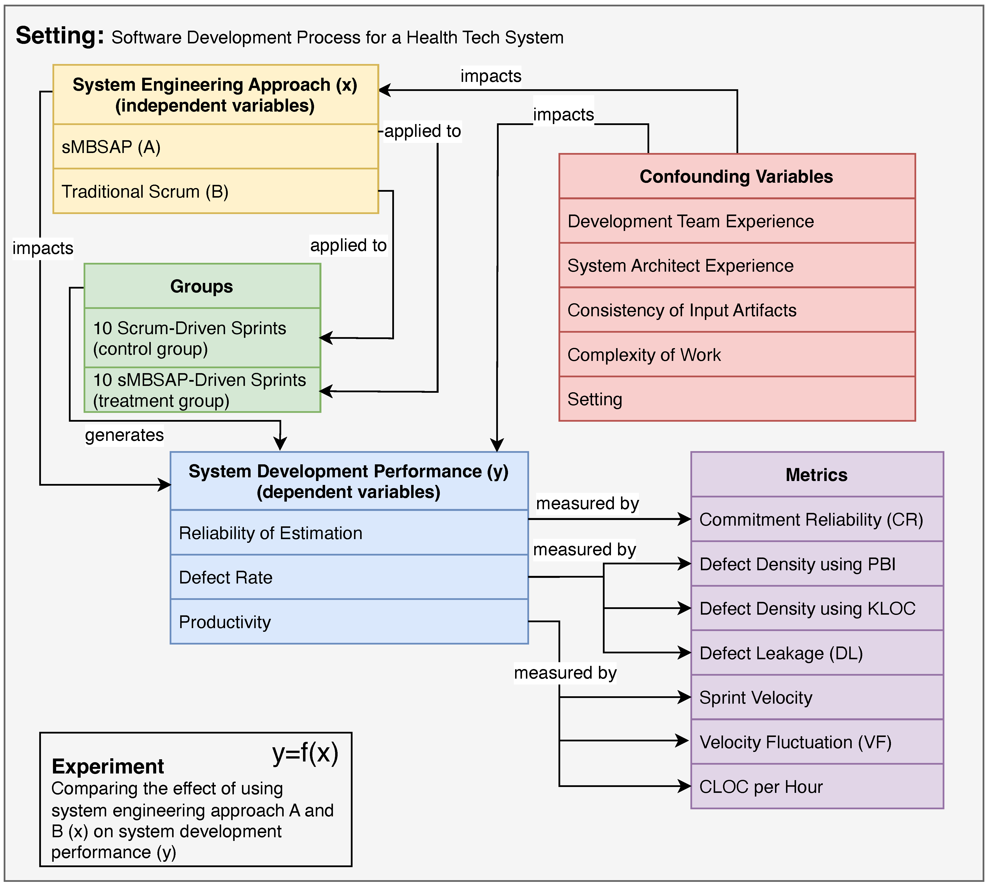
3.1. Experimental Design

In order to explore the differences between sMBSAP and scrum development, here we use an experimental research strategy to probe this comparison. Specifically, we describe the quasi-experimental posttest-only with non-equivalent group studies conducted. The non-equivalent groups’ design was used when the control group and the experimental group did not have pre-experimental sampling equivalence [76,77]. Rather, the groups constituted naturally assembled collectives.
First, all user stories ( m = 260 ) were created and added to a product backlog (Step 1 in Figure 2). Bigger user stories were broken down into tasks (up to 20 tasks per user story). The user stories ( m = 260 ) were reviewed and analyzed to deliver the core system modules (groups of related functions) through sprints ( n = 20 ) (Step 2 in Figure 2). In order to create randomly assigned samples using intact clusters of sprints, all sprints ( n = 20 ) identified in Step 2 were placed into one of two heterogeneous groups (Step 3 in Figure 2). These two groups, containing equal numbers of sprints, were then randomly assigned: one to the treatment group ( n = 10 ) sMBSAP and the other to the control group ( n = 10 ) scrum. These groups were formed in order to avoid the Hawthorn effect [78]. Moreover, the researcher created a model that included a set of viewpoints and perspectives used for both approaches. This artifacts model was created to control one of the confounding variables, that is, “consistency of input artifacts”, by ensuring as many similarities between the sprints as possible.
In scrum, the number of user stories per sprint with a predefined development time window can vary depending on several factors, including team size, the complexity of the stories, and the sprint duration. While there is no strict industry standard or fixed rule of thumb, a commonly recommended guideline is to aim for 5 to 15 user stories per development team member per sprint and assignment of work that is expected to be completed within the given time frame.
The strongest research design for experiments is true experimental design with random sampling from a given population to ensure equivalent groups [76]. Another slightly more elaborate non-equivalent group design, called the pretest–posttest non-equivalent group design, which is used to assess the nature of initial selection differences between the groups and to take account of the effects of these selection differences [77]. However, within the context of this experiment, achieving random assignments without interrupting project delivery and momentum was found to be extremely difficult. The solution researchers offered to address this constraint was assigning the treatment to one intact group or to the other randomly [76,77]. The four steps used in the random assignment of the intact groups for this study are presented in Figure 2.
Now, the dependent variables are the software system development performance objectives, namely, (1) the reliability of estimation, as measured by the C R ; (2) the defect rate, as measured by the D D using the PBI, where the D D is measured using the K L O C and D L ; and (3) the productivity, as measured by the S V , V F , and C L O C p e r h o u r . The experiment overview illustrating the independent, dependent, and confounding variables is shown in Figure 3. This research is a longitudinal study where repeated observations of the same variables were collected for one year (between May 2020 and May 2021). The dependent variables from the executed sprints in both groups ( n = 20 ) were collected and analyzed. Twenty sprints were executed and analyzed for the reliability of estimation and defect rate. All executed sprints were two-week sprints except the last sprint, which was a one-week sprint. To avoid skewing the productivity data, the one-week sprint was excluded from the analysis, so only 19/20 sprints were analyzed (Step 4 in Figure 2).
The research was conducted in a technology startup during the development of a health technology system. The study used the alpha version of the health tech system as the core development effort of the study.

3.2. Techniques and Procedures

There were five main activities (steps) carried out during the quasi-experiment, as explained below.

3.2.1. Step 1: Plan Experiment

The purpose of the first step was to control one of the confounding variables (shown in Figure 3), which was the consistency of the input artifacts. At a high level, these artifacts are the information that the product development ream receives from the system architect at the beginning of a sprint to use in building the software and writing the software code. An architecture framework defining the artifacts for each perspective and the viewpoint of the systems was developed [24]. The framework reduces the threat to validity by ensuring that both the control and treatment groups are as similar as possible by ensuring that the product development team receives comparable artifacts used in writing the software code. In other words, it ensures that both control and treatment groups receive structural, data, behavioral, and requirements artifacts that describe the system.

3.2.2. Step 2: Identify the Metrics for Software Development Performance

Metrics for Reliability of Estimation 

The primary metric used to assess the reliability of estimation is the commitment reliability ( C R ) for each completed sprint:
C R = C o m p l e t e d S P P l a n n e d S P .
In order to assess the C R for all scrum-driven sprints vs. all sMBSAP-driven sprints, the average C R was used. The average C R using a particular approach is defined as follows:
A v e r a g e C R = C R N u m b e r o f S p r i n t s .

Metrics for Productivity 

The primary metric used to assess productivity is S V , which is the sum of the capabilities (features, user stories, requirements, or PBIs) that are successfully delivered in a sprint, which are measured in S P and defined asthe following:
S V = C o m p l e t e d S P D u r i n g a S p r i n t .
In order to assess the S V for all scrum-driven sprints vs. sMBSAP-driven sprints, the average S V was used. The average S V using a particular approach is defined as follows:
A v e r a g e V e l o c i t y = S p r i n t V e l o c i t y N u m b e r o f S p r i n t s .
V F is another way to monitor S V , and it represents the S V variance from the average. Monitoring the V F helps analyze the root cause of the team missing their commitment [56] and is calculated as the following:
V F = A v e r a g e V e l o c i t y S p r i n t V e l o c i t y A v e r a g e V e l o c i t y .
Finally, the total C L O C p e r h o u r was used as a secondary metric to assess productivity:
C L O C p e r h o u r = C L O C D e v e l o p m e n t D u r a t i o n ( h r s ) .

Metrics for Defect Rate 

The primary metric used to assess the defect rate is D D , which is the number of defects found within the PBI executed during a sprint as the following:
D D = D e f e c t C o u n t s ( pre - delivery and post - delivery ) S i z e ( measured in PBI ) ,
where “pre-delivery” defects refer to the defects found during the testing phase, while “post-delivery” defects refer to the defects found after the testing phase.
In order to assess the D D for all dcrum-driven sprints vs. sMBSAP-driven sprints, the average D D was used. The average D D using a particular approach is defined as follows:
A v e r a g e D D = D D N u m b e r o f S p r i n t s .
Another way to calculate the D D is by assessing the number of defects found within the K L O C . The D D using the K L O C approach is calculated as follows:
D D = D e f e c t C o u n t s ( pre - delivery and post - delivery ) S i z e ( measured in KLOC )
Finally, the D L was used as a secondary metric to assess the defect rate. It represents the ratio of defects found during the next phase (post-delivery) vs. the defects found during testing (pre-delivery) and is measured in defects count. Monitoring the D L would help analyze the root cause of leaked defects in order to avoid them before leakage [59] and is calculated as the following:
D L = D e f e c t C o u n t ( post - delivery ) D e f e c t C o u n t ( pre - delivery ) .
In order to assess the D L for all scrum-driven sprints vs. sMBSAP-driven sprints, the average D L was used. The average D L using a particular approach is defined as follows:
A v e r a g e D L = D L N u m b e r o f S p r i n t s .

3.2.3. Step 3: Execute Scrum and sMBSAP Drive Sprints (Scrum and sMBSAP Phases)

The scrum-driven and sMBSAP-driven sprints were executed according to their schedule. The scrum method includes three main components: roles, ceremonies, and artifacts [26]. The scrum processes were grouped into five phases: initiate, plan and estimate, implement, review and retrospect, and release [79]. Also, there were three distinct roles in the scrum process: the product owner, the scrum team, and the scrum master [13]. The scrum method includes periodic meetings known as ceremonies, which include sprint planning, saily scrum (standup), sprint review, and sprint retrospective [22,80,81,82]. In addition to the scrum roles and ceremonies, the scrum process delivers three main artifacts, namely, the product backlog, the sprint backlog, and the product increment [22,80,81,82].
The sMBSAP approach follows a combination of scrum and MBSAP [24]. Two of the four main scrum meetings were used during the sMBSAP approach, namely, daily standups and sprint retro. The other two scrum meetings were modified for sMBSAP. The sprint planning meeting was modified to be a sprint/architecture planning meeting. The same applied to the sprint review meeting, which was modified to be a sprint/architecture review meeting. The typical MBSAP viewpoints generate the architecture artifacts to drive the development process. MBSAP artifacts and sprint backlogs that include user stories are the key information that the product development team uses to execute the product development and show the progress to stakeholders. The sMBSAP [24] approach also included the many typical MBSAP artifacts that included, but were not limited to, a glossary, product breakdown, class diagrams, object diagrams, data model, use-case diagrams, and capabilities. During and at the end of each sprint, the primary data were collected, as explained in the next step.

3.2.4. Step 4: Collect System Development Performance Data

Planning poker [36] and Fibonacci scale [83] techniques were used for planning the amount of work for all sprints. Planning poker is a scrum estimation technique that determines the relative sizing using S P and playing cards [37]. During sprint planning, the PBIs are captured in an agile tool such as ClickUp [84]. During sprint execution, the tracked data elements for each PBI are updated daily. The updated data include the start date, due date, actual closing date, planned S P , and completed S P . At the end of each day, the completed PBIs are marked as“closed”, and the closing date is noted along with the sprint duration. Also, the S P associated with the PBIs were summed up.
The completed S P were plotted on a burnup chart, thus allowing a visual comparison between the ideal and actual progress. At the end of each sprint, the reliability of estimation and productivity metrics were calculated. The data were extracted from ClickUp onto an Excel spreadsheet, which were then imported to PowerBi [85] for analysis and visualization.
To monitor defects, the tester logged the defect under the relevant list using a GitHub repository. Based on the nature of the defect, the tester assigned the defect to a member of the product development team. The product manager reviewed the logged defects, prioritized them, and ensured that each one was assigned to the right person to address that defect. The testers were encouraged to provide as many details as possible when logging a defect on GitHub. They were encouraged to provide steps to reproduce the error, provide screenshots of the defect, and annotate the screenshot for additional clarity. The person who was assigned to a defect may ask questions or add comments, and the tester may respond until the defect is marked as closed and verified by the product manager.
At the end of each sprint, the defects found during testing (pre-delivery) and after passing testing (post-delivery) were captured using GitHub. At the end of the last sprint, the defect-related data points were captured, including sprint duration, PBI, defects captured pre-delivery, defects captured post-delivery, and C L O C .

3.2.5. Step 5: Analyze Data and Compare Results

Descriptive statistics, including means and standard deviations, were used to describe and summarize data to discover emerging patterns. Descriptive data were also used to examine the dispersion of the data sets concerning their mean and standard deviation and were visually inspected using boxplots and bar charts.
The normality test was also used for all three dependent variables [86] to assess the normal distribution. The unpaired t-test was also conducted. The unpaired t-test is a type of inferential statistic that shows how significant the differences between two groups are. In other words, it shows whether those differences (measured in means) could have happened by chance. The t-test is considered to be a robust test against the normality assumption [87,88]. The assumptions required for the independent samples of the t-test were evaluated prior to conducting each t-test and are discussed in Section 3.3.3. The descriptive statistics, normality test, and t-test were performed using GraphPad Prism version 8.0.0 for Mac [89].

3.3. Quality of the Research Design

3.3.1. Minimizing Threats to Reliability

The threats to reliability include an error or bias from the participant’s or researcher’s side. Although the product development team is not the subject of the experiment, the researcher attempted to minimize any error or bias from their side. The researcher identified four sources that could potentially pose threats to reliability: (1) participant error, (2) participant bias, (3) researcher error, and (4) researcher bias. In order to mitigate the first threat, the researcher ensured the control of any factor that could adversely alter how a member of the product development team behaved. As for the second threat, the researcher did not observe any inconsistency in how the product development team planned or executed the sprints. Also, the researcher reviewed all defects detected internally and externally, and no known inconsistencies were observed.
To mitigate the third threat, the researcher did not hesitate to ask the product development team for clarification when the researcher was in doubt during any phase of the experiment. A researcher’s bias may come from any factor that induces bias in the researcher’s input recording [90]. As indicated earlier, given the nature of this quantitative experiment, the interpretation is very limited, and the reliance is mainly on the collected quantitative data. The possibility of the researcher’s bias when recording the data, as they are generated by the product development team, is very limited. For example, when the team reports 20 defects during a sprint, the researcher would record this number without further interpretation from his side.

3.3.2. Minimizing Threats to Validity

A variety of factors may jeopardize experimental and quasi-experimental research’s internal validities. The threats are listed below, along with an explanation of how the researcher sought to reduce them.
  • Selection bias: In this study, some selection bias was introduced by the fact that sprints were chosen to be in one group or the other based on the scheduling of the sprints. The product development team thought it would be counterproductive to execute one sprint using one approach and the following related sprints with the other approach. Although this non-random assignment is considered a threat to internal validity, the benefit of it is that it mitigated the risk of impacting the product development team momentum, which, if occurred, would have affected the productivity measures. Further details on the steps followed to apply random assignment of the intact groups are provided in Section 3.1.
  • Testing effect: Two measures were taken to address this threat. First, having a control group that was executed with scrum helped guard against this threat, since the sprints of the control group were equally subject to the same effect. Second, the researcher did not share with the product development team the details of the study or the specific variables under investigation.
Other threats that were monitored included the history effect, instrumentation effect, and mortality effect. None of these effects were observed or occurred during the experiment. Experimental and quasi-experimental research’s external validities may be also jeopardized by a variety of factors. The factors jeopardizing external validity are listed below, along with the mitigation strategies that the researcher implemented.
  • Changes to the causal relationship due to variations in the implementation within the same approach: During the execution of both groups of sprints, no variations were observed.
  • Interactions of causal relationships with settings: This factor considers the setting in which the cause–effect relationship is measured, thus jeopardizing external validity [91]. The researcher believes that the experimental setting was similar to most development projects after COVID-19, in which team members work and collaborate remotely. However, the research acknowledges that conducting this experiment in other settings would provide further insights into this factor.
  • Interactions of causal relationships with outcomes: This outcome refers to the fact that a cause–effect relationship may exist for one outcome (e.g., more accurate commitment reliability) but not for another seemingly related outcome (e.g., productivity) [92]. The researcher studied the impact of the two approaches on three outcomes. The established causal relation has not been extended from one outcome to another without data collection and measurement, which gives a fuller picture of the treatment’s total impact.
  • The reactive or interactive effect of testing [76]: Given that this quasi-experiment is a posttest only, this factor does not apply to this experiment.

3.3.3. Minimizing Threats to Statistical Conclusion Validity

Examining the dispersion of the data and screening for errors prior to conducting an in-depth analysis is important [93]. All system development performance data were screened for missing items or inconsistencies. To accurately and reliably interpret the test results, some assumptions essential to all data analyses should be proven to be maintained [94]. The assumptions and related tests used before performing the independent samples t-test are considered and discussed in this section. Independent t-tests involve the following assumptions: (1) random assignment, (2) independence, (3) level of measurement, (4) normality and outliers, and (5) homogeneity of variance.
  • Given that the two groups of sprints were not assembled randomly, due to scheduling constraints, the two groups were considered non-equivalent (pre-existing groups). The schedule has been found to play a role in the assignment of subjects to experimental groups in other quasi-experiments in software engineering [95]. In such cases, researchers suggest assigning the treatment to one of the pre-existing (intact) groups or to the other randomly [76,77]. This approach has been borrowed and implemented by researchers in various fields [96], including software engineering [95], and it has also been implemented in this experiment. Therefore, the assumption of the random assignment of intact groups was tenable.
  • The assumption of independence suggests that the data are gathered from groups that are independent of one another [87,97]. In this experiment, special consideration was given to the sequence of the sprint implementation to better ensure that the independence assumption held for the observations within each group. The independence assumption for the t-test refers to the independence of the individual observations within each group rather than the interdependencies between sprints. To best satisfy this assumption, each observation should be unconditionally unrelated and independent of the others in terms of data collection or measurement. Violations of the independence assumption, such as having repeated measures or correlated observations, can lead to biased or incorrect results when using the independent t-test. As an example from the context of this experiment, the number of defects observed in Sprint 6 (a scrum-driven sprint) was independent of that observed in Sprint 7 (also a scrum-driven sprint), and it was also independent of that observed in Sprint 9 (an sMBSAP-driven sprint). A higher or lower number of defects in Sprint 6 had no relationship to the number of defects in Sprints 7 or 8, although there was a schedule interdependency between the three sprints. In summary, while the sprints may have had scheduling dependencies, given that the observations within each group were generally independent of each other, the assumption of independence was tenable for the independent t-test.
  • The dependent variables must be continuous and measured at the interval or ratio scale in order to satisfy the level of measurement assumption for the independent t-test. The level of measurement assumption also requires a categorically independent variable with two groups: one treatment and one control [87]. The type of data collected (ratio scale and interval data) and having had two groups satisfied this assumption.
  • The assumption of normality for each set of system performance data, where the mean was calculated and was visually evaluated, involved the following: first, we used a boxplot to eliminate outliers; then, we used a bar chart; finally, we statistically calculated the data using the normality test [86].
  • Levene’s test was used to assess the argument that there is no difference in the variance of data between groups. A statistically significant value ( 0.05 ) denotes that the assumption has not been satisfied and that the variance between groups is significantly different. Equal variance was not assumed when Levene’s test was significant. Similarly, an equal variance was assumed when Levene’s test was not significant ( p > 0.05 ) [98].

4. Results and Discussion

This section compares the reliability of estimation, productivity, and defect rate metrics from Section 3.2.2 for both the scrum-driven and sMBSAP-driven sprints. The comparisons of the reliability of estimation were conducted based on the results of the C R . The comparisons of the productivity were conducted based on the results of the S V , V F , and C L O C p e r h o u r . Finally, the comparisons of the defect rate were conducted based on the results of the D D and D L . Abbreviations used in this section include the number of samples (N), arithmetic mean (M), and standard deviation ( S D ).

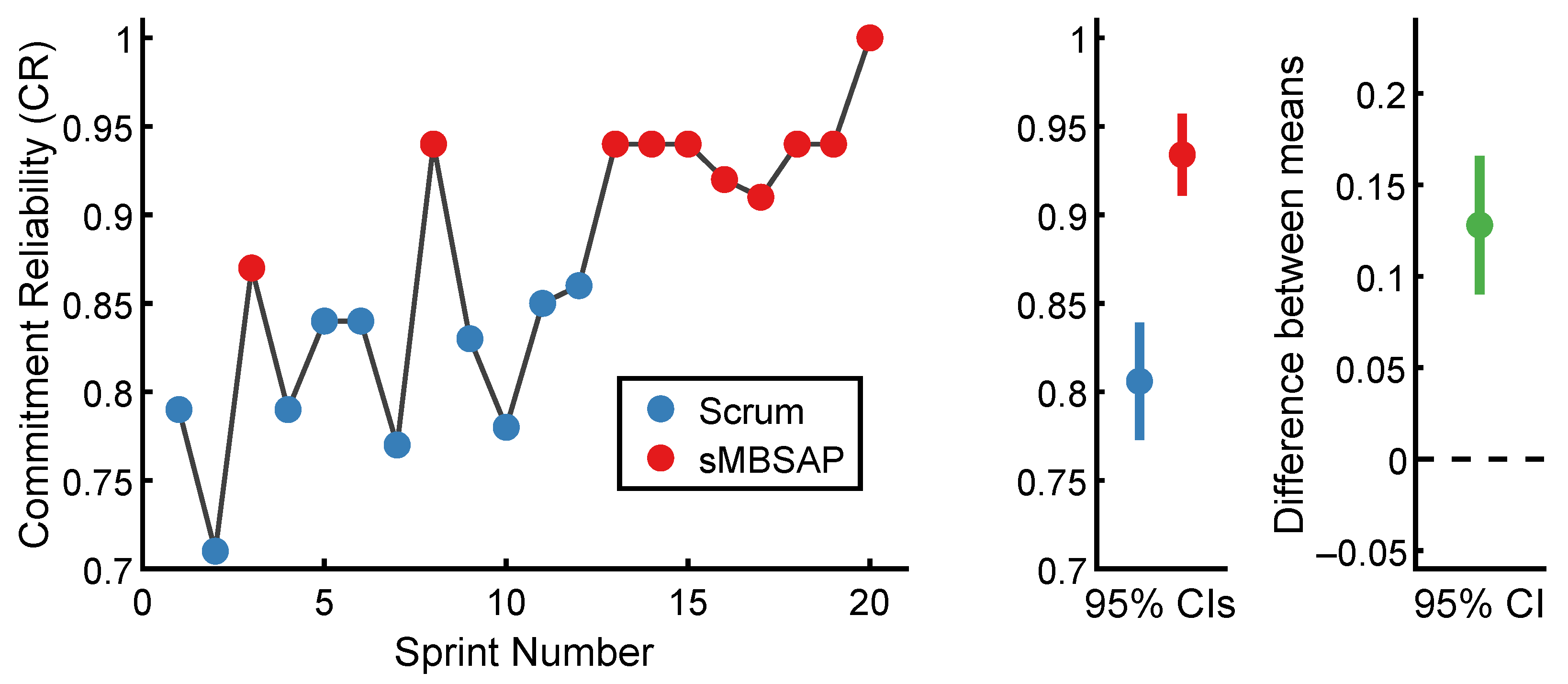
4.1. Reliability of Estimation Results

Commitment Reliability (CR) Comparison

The C R of each sprint in chronological order is presented in Figure 4. For the scrum-driven sprints, the lowest C R was 0.71 for Sprint 2, while the highest C R was 0.86 for Sprint 2. For the sMBSAP-driven sprints, the lowest C R was 0.87 for Sprint 3, while the highest C R was 1.0 for Sprint 20. The scrum-driven sprints ( N = 10 ) were associated with a commitment reliability ratio of M = 0.81 ( S D = 0.046 ). By comparison, the sMBSAP-driven sprints ( N = 10 ) were associated with a numerically larger commitment reliability ratio of M = 0.93 ( S D = 0.032 ). The descriptive statistics are shown in Table 1.
To test the hypothesis that the scrum and sMBSAP were associated with a statistically significantly different mean commitment reliability ratio, an unpaired independent sample t-test was used to compare the scrum-driven sprints and sMBSAP-driven sprints. An alpha level of 0.05 was utilized. The scrum-driven sprint and sMBSAP-driven sprint distributions were sufficiently normal for the purpose of conducting the t-test (i.e., theskew was < | 2.0 | and the Kurtosis was < | 9.0 | [99]). Additionally, the assumption of homogeneity of variance was tested and satisfied via Levene’s F test, thus resulting in F ( 18 ) = 2.059 and p = 0.297 . The independent samples t-test was associated with a statistically significant effect: t ( 18 ) = 7.15 p < 0.0001 0.05 . Thus, the sMBSAP-driven sprints were associated with a statistically significant larger mean commitment reliability than the scrum-driven sprints. A graphical representation of the means and the 95% confidence intervals are displayed in Figure 4.

4.2. Productivity Results

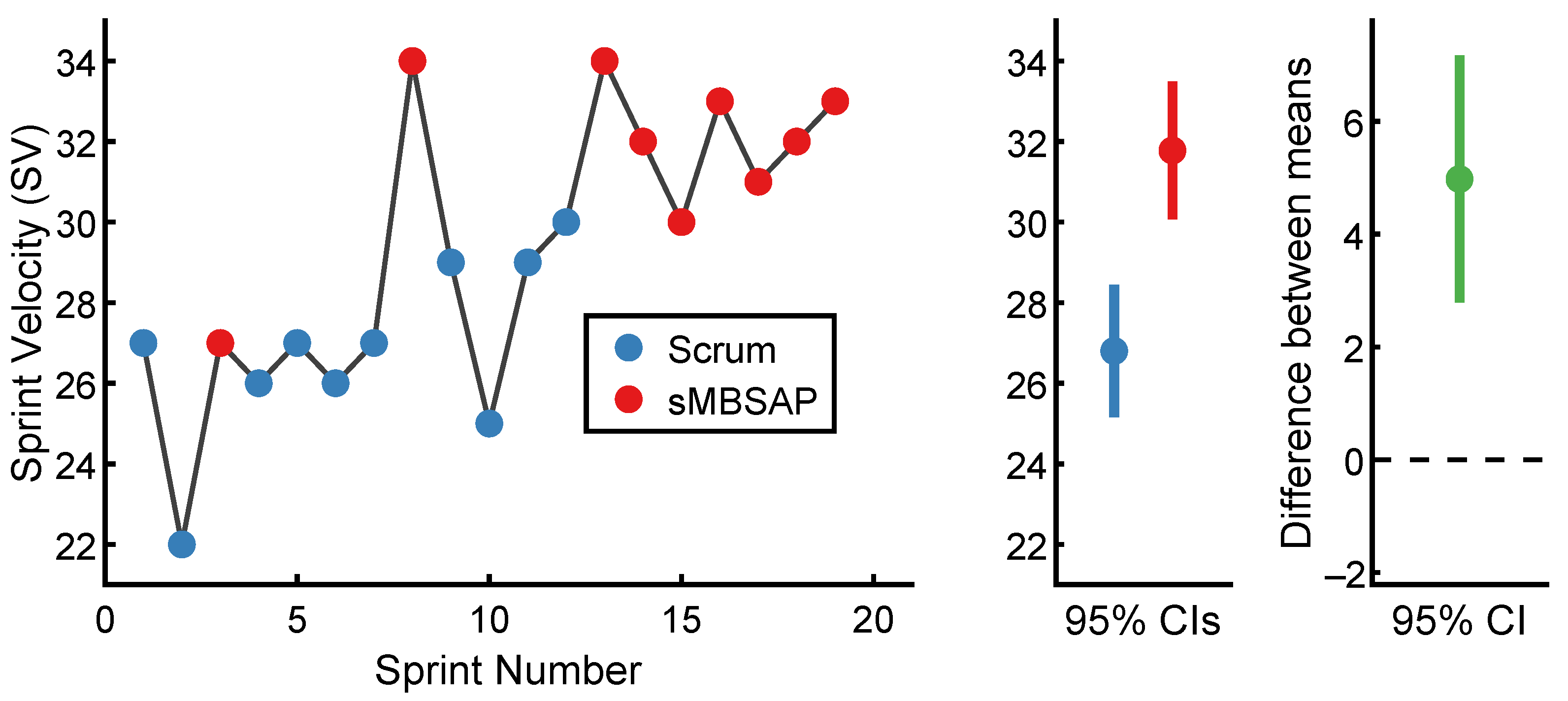
4.2.1. Sprint Velocity (SV) Comparison

The S V of each scrum-driven sprint in chronological order is presented in Figure 5. The lowest S V was 22 for Sprint 2, while the highest S V was 30 for Sprint 12. The scrum-driven sprints ( N = 10 ) were associated with an S V of M = 26.8 ( S D = 2.3 ). Similarly, the S V of each sMBSAP-driven sprint is presented in Figure 5. The lowest S V was 27 for Sprint 3, while the highest S V was 34 for Sprints 8 and 13. By comparison, the sMBSAP-driven sprints ( N = 9 ) were associated with a numerically larger S V of M = 31.8 ( S D = 2.2 ). The descriptive statistics are summarized in Table 2.
To test the hypothesis that the scrum-driven and sMBSAP-driven sprints were associated with a statistically significantly different mean S V , an independent sample t-test was performed. A significance level of 0.05 was utilized. The scrum-driven sprint and sMBSAP-driven sprint distributions were sufficiently normal for the purpose of conducting the t-test (i.e., the | Skew | was < 2.0 and the | Kurtosis | was < 9.0 [99]). Additionally, the required assumption on the homogeneity of variance was tested and satisfied via Levene’s F test, with F ( 17 ) = 1.07 and p = 0.935 . Now, the independent sample t-test was found to be associated with a statistically significant effect: t ( 17 ) = 4.78 p = 0.0002 0.05 . Thus, the sMBSAP-driven sprints were associated with a statistically significant larger mean S V than the scrum-driven sprints. A graphical representation of the means and the 95% confidence intervals are displayed in Figure 5.

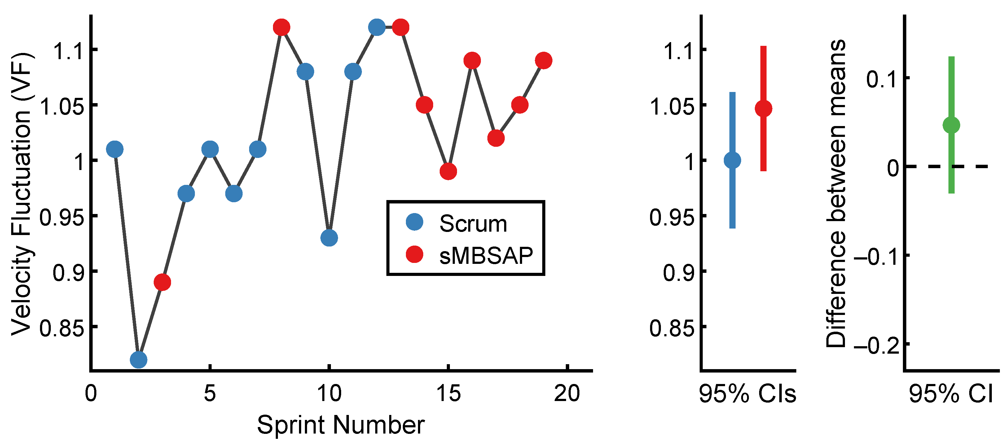
4.2.2. Velocity Fluctuation (VF) Comparison

Based on the captured S V data, the V F of each sprint in chronological order is presented in Figure 6, which was calculated using Equation (5). For the scrum-driven sprints, the lowest V F was 0.82 for Sprint 2, while the highest V F was 1.12 for Sprint 12. For the sMBSAP-driven sprints, the lowest V F was 0.89 for Sprint 3, while the highest V F was 1.12 for Sprints 8 and 13. The scrum-driven sprints ( N = 10 ) were associated with a V F standard deviation ( S D = 0.08 ). By comparison, the sMBSAP-driven sprints ( N = 9 ) were associated with a numerically very similar standard deviation of ( S D = 0.07 ). The descriptive statistics are shown in Table 3. The results from this study suggest no noticeable difference in the V F between the scrum and sMBSAP-driven sprints.

4.2.3. Count of Lines of Code (CLOC) per Hour Comparison

The total C L O C written during the sprints for each approach was used as a secondary measure of the productivity and ended up being approximately 123,000 lines for the dietary recommendation system under consideration. The C L O C written during the scrum-driven sprints was 53,969, while the C L O C written during the sMBSAP-driven sprints was 69,679. The total development hours for the scrum-driven sprints were 930 h, while the total development hours for the sMBSAP-driven sprints were 980 h. Accordingly, and using Equation (6), the C L O C p e r h o u r for the scrum-driven sprints was 58.03. In the same manner, the C L O C p e r h o u r for the sMBSAP-driven sprints was 71.1. Thus, the sMBSAP-driven sprints were associated with a numerically larger C L O C p e r h o u r than the scrum-driven sprints.

4.3. Defect Rate Results

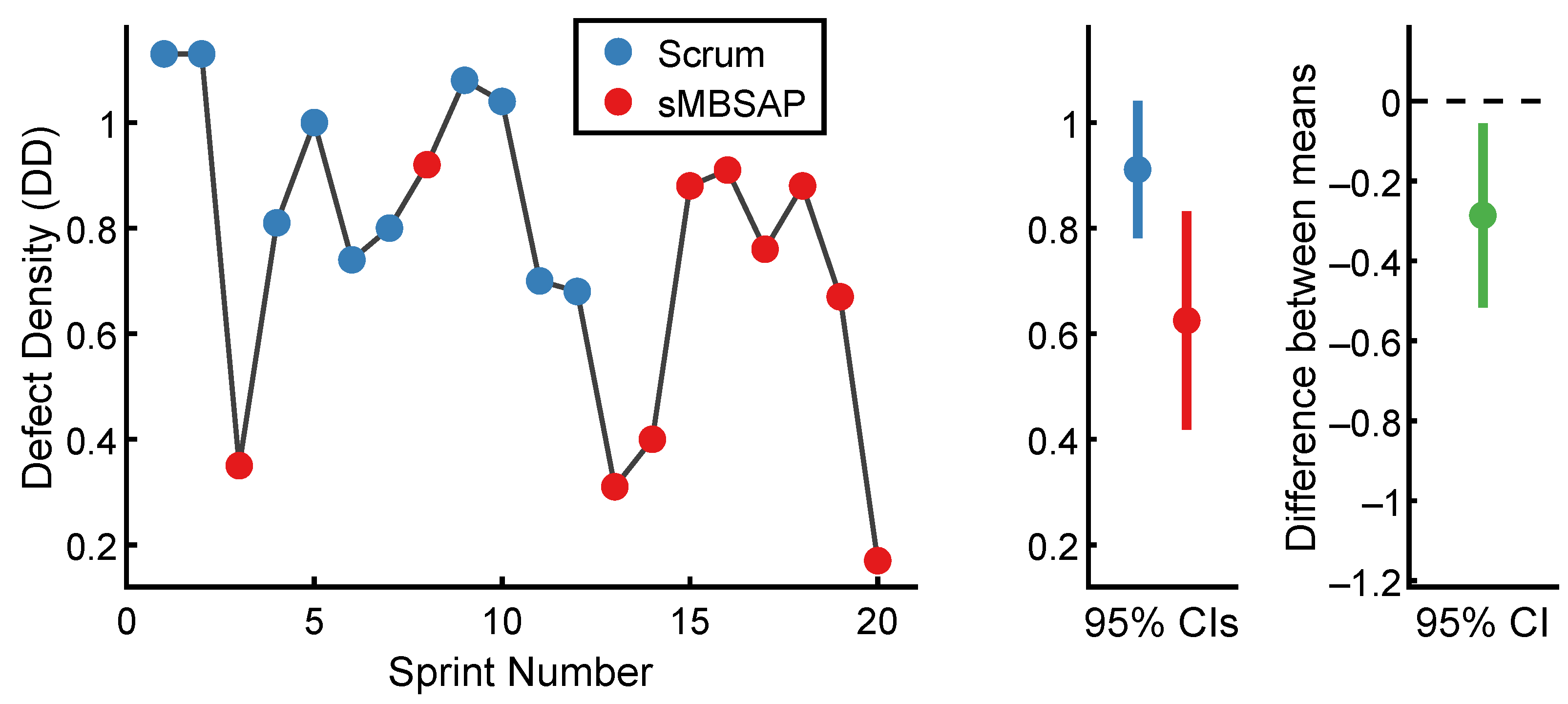
4.3.1. Defect Density (Using PBI) Comparison

Based on the captured defect data and Equation (7), the D D of each sprint is presented in Figure 7. For the scrum-driven sprints, the lowest D D was 0.68 for Sprint 12, while the highest DD was 1.13 for Sprints 1 and 2. For the sMBSAP-driven sprints, the lowest D D was 0.17 for Sprint 20, while the highest D D was 0.92 for Sprint 8. The scrum-driven sprints ( N = 10 ) were associated with a D D of M = 0.91 ( S D = 0.18 ). By comparison, the sMBSAP-driven sprints ( N = 10 ) were associated with a numerically smaller D D of M = 0.63 ( S D = 0.29 ). The descriptive statistics are shown in Table 4.
To test the hypothesis that the scrum-driven and sMBSAP-driven sprints were associated with a statistically significantly different mean D D values, an independent sample t-test was performed. The unpaired t-test was used to compare the D D between the scrum-driven sprints and sMBSAP-driven sprints. An alpha level of 0.05 was utilized. The scrum-driven sprints and sMBSAP-driven sprint distributions were sufficiently normal for the purpose of conducting the t-test (i.e., the skew was < | 2.0 | and the Kurtosis was < | 9.0 | [99]). Additionally, the assumption of homogeneity of variance was tested and satisfied via Levene’s F test, with F ( 18 ) = 2.51 , p = 0.1858 . The independent samples t-test was associated with a statistically significant effect of t ( 18 ) = 2.64 p = 0.016 < 0.05 . Thus, the sMBSAP-driven sprints were associated with a statistically significant smaller mean D D than the scrum-driven sprints. A graphical representation of the means and the 95% confidence intervals are displayed in Figure 7.

4.3.2. Defect Density (within KLOC) Comparison

Based on the captured defect data and Equation (9), the D D of all the scrum-driven sprints (using K L O C ) was 4.57. Similarly, the D D of all the sMBSAP-driven sprints (using K L O C ) was 2.24. The total C L O C written during the sprints for each approach was used as another measure of the size [66]. The C L O C written for developing the dietary recommendation system was approximately 123,000. The C L O C written during the scrum-driven sprints was 53,969, while the C L O C written during the sMBSAP-driven sprints was 69,679. The total number of defects detected during and after the scrum-driven sprints was 247 defects, while the total number of defects detected during and after the sMBSAP-driven sprints was 156 defects. Accordingly, using Equation (9), the defects per K L O C for the scrum-driven sprints was 4.57. In the same manner, the defects per K L O C for the sMBSAP-driven sprints was 2.24. Thus, the sMBSAP-driven sprints were associated with a numerically smaller D D using the C L O C as the size than the scrum-driven sprints.

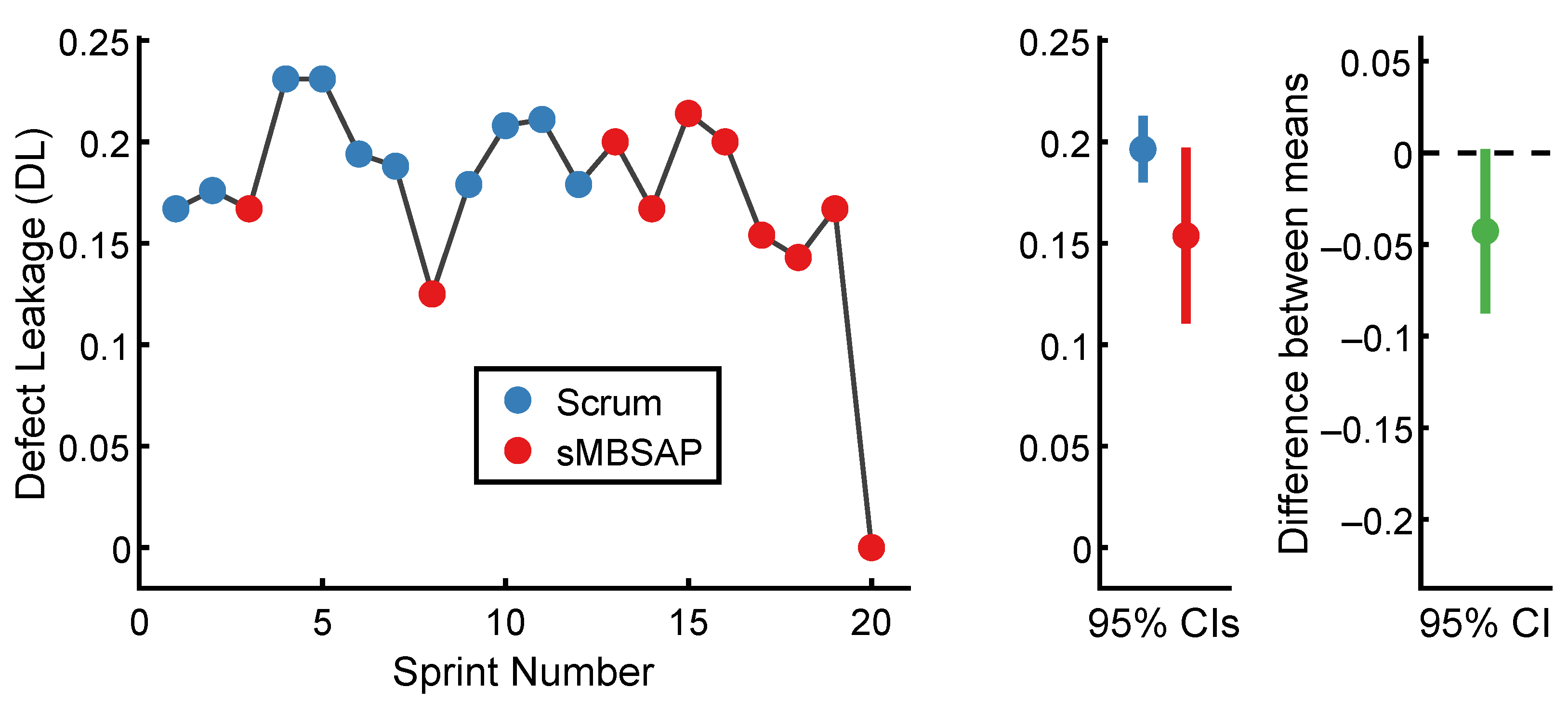
4.3.3. Defect Leakage Comparisons

The D L for each sprint was calculated using Equation (10), and the results are shown in Figure 8. For the scrum-driven sprints, the lowest D L was 16.7% for Sprint 1, while the highest D L was 23.1% for Sprints 4 and 5. Similarly, for the sMBSAP-driven sprints, the lowest D L was 12.5% for Sprint 2, while the highest D L was 21.4% for Sprint 15. The scrum-driven sprints ( N = 10 ) were associated with a D L of M = 0.2 ( S D = 0.02 ). By comparison, the sMBSAP-driven sprints ( N = 10 ) were associated with a numerically smaller D L of M = 0.15 ( S D = 0.06 ). The descriptive statistics are shown in Table 5.
To test the hypothesis that the scrum and sMBSAP-driven sprints were associated with a statistically significantly different mean D L , an independent sample t-test was performed. The unpaired t-test was used to compare the D D between the scrum-driven sprints and sMBSAP-driven sprints. An alpha level of 0.05 was utilized. The scrum-driven sprint and sMBSAP-driven sprint distributions were sufficiently normal for the purpose of conducting the t-test (i.e., the skew was < | 2.0 | and the Kurtosis was < | 9.0 | [99]). Additionally, the assumption of homogeneity of variance was tested and satisfied via Levene’s F test, with F ( 18 ) = 2.51 ,   p = 7.75 . The independent samples t-test was associated with a statistically significant effect, which was t ( 18 ) = 2.13 p = 0.047 < 0.05 . Thus, the sMBSAP-driven sprints were associated with a statistically significant smaller mean D L than the scrum-driven sprints. A graphical representation of the means and the 95% confidence intervals is displayed in Figure 8.

4.3.4. Other Observations

During sprint/architecture planning, it was observed that the product development team reached an agreement on the estimation of the sMBSAP-driven sprints relatively faster than they did for the scrum-driven sprints. The main difference in these meetings was the inputs presented to the team to discuss and conduct their estimations. sMBSAP used a system model as a single repository of the architecture and system requirements [18]. Scrum used multiple tools to capture and present the architecture and system requirements, such as ClickUp [84], Microsoft Office tools [100], and others [101]. The system model seemed to have contributed to making the system architecture and requirements more apparent, unambiguous, and easily communicated with the product development team compared to those of the scrum approach.
The MBSE tool [102] used during the experiment provided methods to create, retrieve, update, and delete the system requirements and architecture content. The tool also aided in generating views of the architecture customized to the product development team needs; the MBSE tool [102] also provided simulation capabilities of the architecture to support analysis and evaluation. In summary, the main benefit observed from using a model resided in its ability to visually represent the end-to-end software development flow from user needs to delivered and supported software solutions. It was also observed, during the daily standups and the sprint/architecture review, that the product development team demonstrated more of a grasp of the features and functions that needed to be developed. Although both the scrum and sMBSAP aim at improving productivity, the visual representation capabilities of the sMBSAP gave it a comparative advantage.
The repeatable activities using architecture modeling and screen wireframing built-in within the model as the foundation contributed to unambiguous communication with the product development team. The visually clear direction seems to have improved the capability of the product development team to interpret the features and functions, accordingly, which helped to complete more S P within the same time frame and with fewer defects. Finally, using the architecture model to highlight the completed parts of the system effectively communicated the progress of the development effort. Similarly, using the architecture model to highlight the parts of the system based on their defect rate effectively communicated the defect status.

5. Conclusions and Future Work

The purpose of this study was to compare the software development performance of the sMBSAP vs. that of the scrum. Investigating the relative value of an agile MBSE approach over agile alone might solve one of the obstacles to the adoption of agile MBSE.
Towards this goal, results were collected from a quasi-experimental posttest-only with non-equivalent group research designs for the software development of a health technology system. The independent variables were the two software development methods, the sMBSAP and scrum, which were actuated during different development sprints. The dependent variables were the software system development performance objectives of (1) the reliability of estimation as measured by C R ; (2) the defect rate as measured by D D using PBI, K L O C , and D L ; and (3) the productivity as measured by S V , V F , and C L O C p e r h o u r . A total of twenty sprints were executed, with ten sprints executed for each approach, respectively.
From the results, the observed commitment reliability and productivity for the sMBSAP-driven sprints were larger than those of the scrum-driven sprints, and the observed defect rate for the sMBSAP-driven sprints was smaller than that of the scrum-driven sprints. Specifically, it was observed that there was a 16% increase in the C R , a 13.4% increase in the S V , a 22.5% increase in the C L O C p e r h o u r , a 31.8% decrease in the D D using the PBIs method, a 50% decrease in the D D using the KLOC method, and a 21.4% decrease in the D L .
The improved reliability of estimation, productivity, and defect rate could potentially help reduce the risk of running behind schedule and overbudgetting that can occur with agile-driven projects. Overall, these results provide some evidence of the efficacy of a combined agile MBSE approach in managing software-based systems and in strengthening the case for its adoption within the software development community, as well as the broader systems engineering community.
The factors that pose threats to reliability, validity, and statistical conclusion validity have been identified, monitored, and mitigated to minimize the impact of these factors on the quality of the research design. However, there are still aspects of the research design that could be improved to provide additional clear and convincing evidence regarding the relative value of agile MBSE approaches. There is a need for deeper comparative analyses between agile and agile MBSE methods using other software development objectives, techniques, and metrics beyond the ones included in this study. Future work, then, might also include comparative analysis for software products in industries other than health technology against agile methodologies other than scrum, as well as for different sizes of projects and teams. Such work would provide additional insights for the software development community.
Domain-specific software engineering is an emerging paradigm that has the potential to improve both the correctness and reliability of the software system and also lead to greater opportunities for software automation. Future work may consider leveraging the capabilities of agile MBSE methods such as sMBSAP in domain-specific software engineering, such as blockchain-orientated software development [103].
Finally, due to several practical limitations, this study did not pursue a true experimental design (and this is likely the case for many software development research activities). However, a potential direction may include developing the same product along two parallel tracks (i.e., developing the same product twice): one track could use an agile MBSE, and the other could use an agile approach. Even if a single track might be used (i.e., developing the product once, as was done in this study), the researcher might consider a true experimental design with random sampling from a given population when assigning an approach to a given sprint. However, care must be taken to ensure that such a non-traditional development plan does not adversely impact the momentum and other factors.

Author Contributions

Conceptualization, M.H., J.M.B. and D.R.H.; methodology, M.H.; software, M.H.; validation, D.R.H.; formal analysis, M.H.; investigation M.H.; data curation, M.H.; writing—original draft preparation, M.H.; writing—review and editing, D.R.H.; visualization, M.H. and D.R.H.; supervision, D.R.H. and J.M.B. All authors have read and agreed to the published version of the manuscript.

Funding

This research received no external funding.

Data Availability Statement

The reliability of estimation, productivity, and defect rate data presented in this study are available on request from the corresponding author. The data will be made publicly available upon publishing the dissertation of the corresponding author.

Conflicts of Interest

The lead author is one of the co-founders of Hekafy Inc., the startup company which developed the health tech app in this research study.

Abbreviations

The following abbreviations are used in this manuscript:
C L O C     Count of Lines of Code
C R Commitment Reliability
DBSEDocument-Based Systems Engineering
D D Defect Density
D L Defect Leakage
EVEarned Value
K L O C Thousands (Kilo) of Lines of Code
MArithmetic Mean
MBSAPModel-Based System Architecture Process
MBSEModel-Based Software Engineering
NNumber of Samples
PBIProduct Backlog Items
ROIReturn-On-Investment
S D Standard Deviation
sMBSAPScrum Model-Based System Architecture Process
S P Story Points
S V Sprint Velocity
V F Velocity Fluctuation

References

  1. Tohidi, H. The role of risk management in IT systems of organizations. Procedia Comput. Sci. 2011, 3, 881–887. [Google Scholar] [CrossRef] [Green Version]
  2. Standish Group. CHAOS Report 2020; Technical Report; Standish Group: Boston, MA, USA, 2020. [Google Scholar]
  3. Altahtooh, U.A.; Emsley, M.W. Is a Challenged Project One of the Final Outcomes for an IT Project? In Proceedings of the 2014 47th Hawaii International Conference on System Sciences, Waikoloa, HI, USA, 6–9 January 2014; pp. 4296–4304. [Google Scholar] [CrossRef]
  4. Muganda Ochara, N.; Kandiri, J.; Johnson, R. Influence processes of implementation effectiveness in challenged information technology projects in Africa. Inf. Technol. People 2014, 27, 318–340. [Google Scholar] [CrossRef]
  5. Yeo, K.T. Critical failure factors in information system projects. Int. J. Proj. Manag. 2022, 20, 241–246. [Google Scholar] [CrossRef]
  6. Bloch, M.; Blumberg, S.; Laartz, J. Delivering large-scale IT projects on time, on budget, and on value. Harv. Bus. Rev. 2012, 5, 2–7. [Google Scholar]
  7. Flyvbjerg, B.; Budzier, A. Why Your IT Project May Be Riskier Than You Think. Harv. Bus. Rev. 2011, 89, 23–25. [Google Scholar] [CrossRef]
  8. Eadicicco, L.; Peckham, M.; Pullen, J.P.; Fitzpatrick, A. Time The 20 Most Successful Tech Failures of All Time. Time. 2017. Available online: https://time.com/4704250/most-successful-technology-tech-failures-gadgets-flops-bombs-fails/ (accessed on 15 September 2019).
  9. Martin, J. Rapid Application Development; Macmillan Publishing Co., Inc.: New York, NY, USA, 1991. [Google Scholar]
  10. Ambler, S. The Agile Unified Process (Aup). 2005. Available online: http://www.ambysoft.com/unifiedprocess/agileUP.html (accessed on 10 March 2023).
  11. Turner, R. Toward Agile systems engineering processes. J. Def. Softw. Eng. 2007, 11–15. Available online: https://citeseerx.ist.psu.edu/document?repid=rep1&type=pdf&doi=b807d8efe4acd265187a98357b19c063b5a9ad5e (accessed on 15 April 2020).
  12. Schwaber, K. Scrum development process. In Business Object Design And Implementation; OOPSLA ’95 Workshop Proceedings, Austin, TX, USA, 16 October 1995; Springer: Berlin/Heidelberg, Germany, 1997; pp. 117–134. [Google Scholar]
  13. Akif, R.; Majeed, H. Issues and challenges in Scrum implementation. Int. J. Sci. Eng. Res. 2012, 3, 1–4. [Google Scholar]
  14. Cardozo, E.S.F.; Araújo Neto, J.B.F.; Barza, A.; França, A.C.C.; da Silva, F.Q.B. Scrum and productivity in software projects: A systematic literature review. In Proceedings of the International Conference on Evaluation and Assessment in Software Engineering, Keele, UK, 12–13 April 2010. [Google Scholar] [CrossRef]
  15. Lehman, T.; Sharma, A. Software development as a service: Agile experiences. In Proceedings of the 2011 Annual SRII Global Conference, San Jose, CA, USA, 29 March–2 April 2011; pp. 749–758. [Google Scholar]
  16. ISO/IEC/IEEE 15288:2023; Systems and Software Engineering—System Life Cycle Processes. ISO, IEC, and IEEE: Geneva, Switzerland, 2023. [CrossRef]
  17. Dove, R.; Schindel, W. Agility in Systems Engineering—Findings from Recent Studies; Working Paper; Paradigm Shift International and ICTT System Sciences: 2017. Available online: http://www.parshift.com/s/ASELCM-AgilityInSE-RecentFindings.pdf (accessed on 12 April 2020).
  18. Henderson, K.; Salado, A. Value and benefits of model-based systems engineering (MBSE): Evidence from the literature. Syst. Eng. 2021, 24, 51–66. [Google Scholar] [CrossRef]
  19. Douglass, B.P. Agile Model-Based Systems Engineering Cookbook, 1st ed.; Packt Publishing: Birmingham, UK, 2021. [Google Scholar]
  20. Salehi, V.; Wang, S. Munich Agile MBSE concept (MAGIC). Int. Conf. Eng. Des. 2019, 1, 3701–3710. [Google Scholar] [CrossRef] [Green Version]
  21. Riesener, M.; Doelle, C.; Perau, S.; Lossie, P.; Schuh, G. Methodology for iterative system modeling in Agile product development. Procedia CIRP 2021, 100, 439–444. [Google Scholar] [CrossRef]
  22. Bott, M.; Mesmer, B. An analysis of theories supporting Agile Scrum and the use of Scrum in systems engineering. Eng. Manag. J. 2020, 32, 76–85. [Google Scholar] [CrossRef]
  23. Ciampa, P.D.; Nagel, B. Accelerating the development of complex systems in aeronautics via MBSE and MDAO: A roadmap to agility. In Proceedings of the AIAA AVIATION Forum and Exposition, Number AIAA 2021-3056. Virtual Event, 2–6 August 2021. [Google Scholar] [CrossRef]
  24. Huss, M.; Herber, D.R.; Borky, J.M. An Agile model-based software engineering approach illustrated through the development of a health technology system. Software 2023, 2, 234–257. [Google Scholar] [CrossRef]
  25. Borky, J.M.; Bradley, T.H. Effective Model-Based Systems Engineering; Springer: Berlin/Heidelberg, Germany, 2019. [Google Scholar] [CrossRef]
  26. Schwaber, K. Agile Project Management with Scrum; Microsoft Press: Redmond, WA, USA, 2004. [Google Scholar]
  27. Anand, R.V.; Dinakaran, M. Issues in Scrum Agile development principles and practices in software development. Indian J. Sci. Technol. 2015, 8, 1–5. [Google Scholar] [CrossRef]
  28. Brambilla, M.; Cabot, J.; Wimmer, M. Model-Driven Software Engineering in Practice; Springer: Berlin/Heidelberg, Germany, 2017. [Google Scholar] [CrossRef]
  29. Bonnet, S.; Voirin, J.L.; Normand, V.; Exertier, D. Implementing the MBSE cultural change: Organization, coaching and lessons learned. In Proceedings of the INCOSE International Symposium, Seattle, WA, USA, 13–16 July 2015; Volume 25, pp. 508–523. [Google Scholar] [CrossRef]
  30. Azhar, D.; Mendes, E.; Riddle, P. A systematic review of web resource estimation. In Proceedings of the International Conference on Predictive Models in Software Engineering, Lund, Sweden, 21–22 September 2012; pp. 49–58. [Google Scholar] [CrossRef]
  31. Jorgensen, M.; Shepperd, M. A systematic review of software development cost estimation studies. IEEE Trans. Softw. Eng. 2006, 33, 33–53. [Google Scholar] [CrossRef] [Green Version]
  32. Molokken, K.; Jorgensen, M. A review of software surveys on software effort estimation. In Proceedings of the International Symposium on Empirical Software Engineering, Rome, Italy, 30 September–1 October 2003; pp. 223–230. [Google Scholar] [CrossRef]
  33. Wen, J.; Li, S.; Lin, Z.; Hu, Y.; Huang, C. Systematic literature review of machine learning based software development effort estimation models. Inf. Softw. Technol. 2012, 54, 41–59. [Google Scholar] [CrossRef]
  34. Cohn, M. Agile Estimating and Planning; Pearson Education: Harlow, UK, 2005. [Google Scholar]
  35. Grenning, J. Planning Poker or How to Avoid Analysis Paralysis While Release Planning; White Paper; Renaissance Software Consulting: Hawthorn Woods, IL, USA, 2002. [Google Scholar]
  36. Mahnič, V.; Hovelja, T. On using planning poker for estimating user stories. J. Syst. Softw. 2012, 85, 2086–2095. [Google Scholar] [CrossRef]
  37. Dalton, J. Planning Poker. In Great Big Agile; Springer: Berlin/Heidelberg, Germany, 2019; pp. 203–204. [Google Scholar] [CrossRef]
  38. Haugen, N.C. An empirical study of using planning poker for user story estimation. In Proceedings of the AGILE, Minneapolis, MN, USA, 23–28 July 2006. [Google Scholar] [CrossRef]
  39. Moløkken-Østvold, K.; Haugen, N.C.; Benestad, H.C. Using planning poker for combining expert estimates in software projects. J. Syst. Softw. 2008, 81, 2106–2117. [Google Scholar] [CrossRef]
  40. Molokken-Østvold, K.; Haugen, N.C. Combining estimates with planning poker–An empirical study. In Proceedings of the Australian Software Engineering Conference, Melbourne, Australia, 10–13 April 2007; pp. 349–358. [Google Scholar] [CrossRef]
  41. Moløkken-Østvold, K.; Jørgensen, M.; Tanilkan, S.S.; Gallis, H.; Lien, A.C.; Hove, S.W. A survey on software estimation in the Norwegian industry. In Proceedings of the International Symposium on Software Metrics, Chicago, IL, USA, 11–17 September 2004; pp. 208–219. [Google Scholar] [CrossRef]
  42. Tiwari, M. Understanding Scrum Metrics and KPIs. Online, 2019. Medium. Available online: https://medium.com/@techiemanoj4/understanding-scrum-metrics-and-kpis-fcf56833d488 (accessed on 12 April 2020).
  43. Smart, J. To transform to have agility, dont do a capital A, capital T Agile transformation. IEEE Softw. 2018, 35, 56–60. [Google Scholar] [CrossRef]
  44. Khanzadi, M.; Shahbazi, M.M.; Taghaddos, H. Forecasting schedule reliability using the reliability of agents’ promises. Asian J. Civ. Eng. 2018, 19, 949–962. [Google Scholar] [CrossRef]
  45. Chen, C.; Housley, S.; Sprague, P.; Goodlad, P. Introducing lean into the UK Highways Agency’s supply chain. Proc. Inst. Civ. Eng.-Civ. Eng. 2012, 165, 34–39. [Google Scholar] [CrossRef]
  46. Wagner, S.; Ruhe, M. A systematic review of productivity factors in software development. arXiv 2018, arXiv:1801.06475. [Google Scholar] [CrossRef]
  47. Maxwell, K.; Forselius, P. Benchmarking software development productivity. IEEE Softw. 2000, 17, 80–88. [Google Scholar] [CrossRef] [Green Version]
  48. Brodbeck, F.C. Produktivität und Qualität in Software-Projekten: Psychologische Analyse und Optimierung von Arbeitsprozessen in der Software-Entwicklung; Oldenbourg: München, Germany, 1994. [Google Scholar]
  49. Kitchenham, B.; Mendes, E. Software productivity measurement using multiple size measures. IEEE Trans. Softw. Eng. 2004, 30, 1023–1035. [Google Scholar] [CrossRef]
  50. Huijgens, H.; Solingen, R.v. A replicated study on correlating agile team velocity measured in function and story points. In Proceedings of the International Workshop on Emerging Trends in Software Metrics, Hyderabad, India, 3 June 2014; pp. 30–36. [Google Scholar] [CrossRef]
  51. Alleman, G.B.; Henderson, M.; Seggelke, R. Making Agile development work in a government contracting environment-measuring velocity with earned value. In Proceedings of the Agile Development Conference, Salt Lake City, UT, USA, 25–28 June 2003; pp. 114–119. [Google Scholar] [CrossRef]
  52. Javdani, T.; Zulzalil, H.; Ghani, A.A.A.; Sultan, A.B.M.; Parizi, R.M. On the current measurement practices in Agile software development. arXiv 2013, arXiv:1301.5964. [Google Scholar] [CrossRef]
  53. Kupiainen, E.; Mäntylä, M.V.; Itkonen, J. Using metrics in Agile and lean software development–a systematic literature review of industrial studies. Inf. Softw. Technol. 2015, 62, 143–163. [Google Scholar] [CrossRef]
  54. Killalea, T. Velocity in software engineering. Commun. ACM 2019, 62, 44–47. [Google Scholar] [CrossRef]
  55. Sharma, S.; Kumar, D.; Fayad, M.E. An impact assessment of Agile ceremonies on sprint velocity under Agile software development. In Proceedings of the International Conference on Reliability, Infocom Technologies and Optimization (Trends and Future Directions), Noida, India, 3–4 September 2021. [Google Scholar] [CrossRef]
  56. Albero Pomar, F.; Calvo-Manzano, J.A.; Caballero, E.; Arcilla-Cobián, M. Understanding sprint velocity fluctuations for improved project plans with Scrum: A case study. J. Softw. Evol. Process. 2014, 26, 776–783. [Google Scholar] [CrossRef] [Green Version]
  57. IEEE Std 610 12; IEEE Standard Glossary of Software Engineering Terminology. IEEE: New York, NY, USA, 1990. [CrossRef]
  58. Tripathy, P.; Naik, K. Software Testing and Quality Assurance: Theory and Practice; John Wiley & Sons: New York, NY, USA, 2011. [Google Scholar] [CrossRef]
  59. McDonald, M.; Musson, R.; Smith, R. The Practical Guide to Defect Prevention; Microsoft Press: Hong Kong, China, 2007. [Google Scholar]
  60. Jones, C.; Bonsignour, O. The Economics of Software Quality; Addison-Wesley Professional: Boston, MA, USA, 2011. [Google Scholar]
  61. Boehm, B. Get ready for Agile methods, with care. Computer 2002, 35, 64–69. [Google Scholar] [CrossRef] [Green Version]
  62. Boehm, B.; Basili, V.R. Top 10 list [software development]. Computer 2001, 34, 135–137. [Google Scholar] [CrossRef]
  63. Song, Q.; Jia, Z.; Shepperd, M.; Ying, S.; Liu, J. A general software defect-proneness prediction framework. IEEE Trans. Softw. Eng. 2010, 37, 356–370. [Google Scholar] [CrossRef] [Green Version]
  64. Mohagheghi, P.; Conradi, R.; Killi, O.M.; Schwarz, H. An empirical study of software reuse vs. defect-density and stability. In Proceedings of the International Conference on Software Engineering, Beijing, China, 30 September 2004; pp. 282–291. [Google Scholar] [CrossRef] [Green Version]
  65. Nagappan, N.; Ball, T. Use of relative code churn measures to predict system defect density. In Proceedings of the International Conference on Software Engineering, St. Louis, MO, USA, 15–21 May 2005; pp. 284–292. [Google Scholar] [CrossRef]
  66. Shah, S.M.A.; Morisio, M.; Torchiano, M. An overview of software defect density: A scoping study. In Proceedings of the Asia-Pacific Software Engineering Conference, Hong Kong, China, 4–7 December 2012; Volume 1, pp. 406–415. [Google Scholar] [CrossRef]
  67. Mijumbi, R.; Okumoto, K.; Asthana, A.; Meekel, J. Recent advances in software reliability assurance. In Proceedings of the IEEE International Symposium on Software Reliability Engineering Workshops, Memphis, TN, USA, 15–18 October 2018; pp. 77–82. [Google Scholar] [CrossRef]
  68. Fehlmann, T.M.; Kranich, E. Measuring defects in a six sigma context. In Proceedings of the International Conference on Lean Six Sigma, Durgapur, India, 9–11 January 2014. [Google Scholar]
  69. Li, J.; Moe, N.B.; Dybå, T. Transition from a plan-driven process to Scrum: A longitudinal case study on software quality. In Proceedings of the ACM-IEEE International Symposium on Empirical Software Engineering and Measurement, Bolzano-Bozen, Italy, 16–17 September 2010. [Google Scholar] [CrossRef]
  70. Collofello, J.S.; Yang, Z.; Tvedt, J.D.; Merrill, D.; Rus, I. Modeling software testing processes. In Proceedings of the IEEE Fifteenth Annual International Phoenix Conference on Computers and Communications, Scottsdale, AZ, USA, 27–29 March 1996; pp. 289–293. [Google Scholar] [CrossRef] [Green Version]
  71. Jacob, P.M.; Prasanna, M. A comparative analysis on black box testing strategies. In Proceedings of the International Conference on Information Science, Dublin, Ireland, 11–14 December 2016; pp. 1–6. [Google Scholar] [CrossRef]
  72. Rawat, M.S.; Dubey, S.K. Software defect prediction models for quality improvement: A literature study. Int. J. Comput. Sci. Issues 2012, 9, 288–296. [Google Scholar]
  73. Vashisht, V.; Lal, M.; Sureshchandar, G.S. A framework for software defect prediction using neural networks. J. Softw. Eng. Appl. 2015, 8, 384–394. [Google Scholar] [CrossRef]
  74. Carroll, E.R.; Malins, R.J. Systematic Literature Review: HOW Is Model-Based Systems Engineering Justified? Technical Report SAND2016-2607; Sandia National Laboratories: Albuquerque, NM, USA, 2016. [Google Scholar] [CrossRef] [Green Version]
  75. Friedenthal, S.; Moore, A.; Steiner, R. A Practical Guide to SysML; Morgan Kaufmann: San Francisco, CA, USA, 2014. [Google Scholar] [CrossRef]
  76. Campbell, D.T.; Stanley, J.C. Experimental and Quasi-Experimental Designs for Research; Houghton Mifflin Company: Boston, MA, USA, 1963. [Google Scholar]
  77. Reichardt, C.S. Quasi-Experimentation: A Guide to Design and Analysis; Guilford Publications: New York, NY, USA, 2019. [Google Scholar]
  78. Schwartz, D.; Fischhoff, B.; Krishnamurti, T.; Sowell, F. The Hawthorne effect and energy awareness. Proc. Natl. Acad. Sci. USA 2013, 110, 15242–15246. [Google Scholar] [CrossRef]
  79. Satpathy, T.; et al. A Guide to the Scrum Body of Knowledge (SBOK™ Guide), 3rd ed.; SCRUMstudy: Avondale, AZ, USA, 2016. [Google Scholar]
  80. Buffardi, K.; Robb, C.; Rahn, D. Learning agile with tech startup software engineering projects. In Proceedings of the ACM Conference on Innovation and Technology in Computer Science Education, Bologna, Italy, 3–5 July 2017; pp. 28–33. [Google Scholar] [CrossRef]
  81. Ghezzi, A.; Cavallo, A. Agile business model innovation in digital entrepreneurship: Lean startup approaches. J. Bus. Res. 2020, 110, 519–537. [Google Scholar] [CrossRef]
  82. Kuchta, D. Combination of the earned value method and the Agile approach—A case study of a production system implementation. In Proceedings of the Intelligent Systems in Production Engineering and Maintenance, Wroclaw, Poland, 17–18 September 2018; pp. 87–96. [Google Scholar] [CrossRef]
  83. Tamrakar, R.; Jørgensen, M. Does the use of Fibonacci numbers in planning poker affect effort estimates? In Proceedings of the International Conference on Evaluation & Assessment in Software Engineering, Ciudad Real, Spain, 14–15 May 2012. [Google Scholar] [CrossRef] [Green Version]
  84. ClickUp™. Available online: https://www.clickup.com (accessed on 28 February 2023).
  85. Powerbi™. Available online: https://powerbi.microsoft.com/en-us/ (accessed on 28 February 2023).
  86. Das, K.R.; Imon, A. A brief review of tests for normality. Am. J. Theor. Appl. Stat. 2016, 5, 5–12. [Google Scholar] [CrossRef] [Green Version]
  87. Rovai, A.P.; Baker, J.D.; Ponton, M.K. Social Science Research Design and Statistics; Watertree Press: Long Beach, CA, USA, 2013. [Google Scholar]
  88. Rasch, D.; Teuscher, F.; Guiard, V. How robust are tests for two independent samples? J. Stat. Plan. Inference 2007, 137, 2706–2720. [Google Scholar] [CrossRef]
  89. Prism™. Available online: https://www.graphpad.com/ (accessed on 28 February 2023).
  90. Saunders, M.; Lewis, P.; Thornhill, A. Research Methods, 8th ed.; Pearson Education: Upper Saddle River, NJ, USA, 2019. [Google Scholar]
  91. Cook, T.D.; Reichardt, C.S. Qualitative and Quantitative Methods in Evaluation Research; Sage Publications: Thousand Oaks, CA, USA, 1979. [Google Scholar]
  92. Matthay, E.C.; Glymour, M.M. A graphical catalog of threats to validity: Linking social science with epidemiology. Epidemiology 2020, 31, 376–384. [Google Scholar] [CrossRef]
  93. Howell, D.C. Chi-square test: Analysis of contingency tables. In International Encyclopedia of Statistical Science; Springer: Berlin/Heidelberg, Germany, 2011; pp. 250–252. [Google Scholar] [CrossRef]
  94. Field, A. Discovering Statistics Using IBM SPSS Statistics; Sage: Thousand Oaks, CA, USA, 2013. [Google Scholar]
  95. Kampenes, V.B.; Dybå, T.; Hannay, J.E.; Sjøberg, D.I. A systematic review of quasi-experiments in software engineering. Inf. Softw. Technol. 2009, 51, 71–82. [Google Scholar] [CrossRef]
  96. Gall, M.D.; Gall, J.P.; Borg, W.R. Educational Research: An Introduction; Pearson: Upper Saddle River, NJ, USA, 2007. [Google Scholar]
  97. Field, A.P. Is the meta-analysis of correlation coefficients accurate when population correlations vary? Psychol. Methods 2005, 10, 444–467. [Google Scholar] [CrossRef] [Green Version]
  98. Gastwirth, J.L.; Gel, Y.R.; Miao, W. The impact of Levene’s test of equality of variances on statistical theory and practice. Stat. Sci. 2009, 24, 343–360. [Google Scholar] [CrossRef] [Green Version]
  99. Schmider, E.; Ziegler, M.; Danay, E.; Beyer, L.; Bühner, M. Is it really robust? Methodology 2010, 6, 147–151. [Google Scholar] [CrossRef]
  100. Microsoft 365. Available online: https://www.office.com (accessed on 28 February 2023).
  101. Diagrams.net. Draw.io. Available online: https://draw.io (accessed on 28 February 2023).
  102. Sparx Systems. Enterprise Architect 15.2 User Guide. Available online: https://sparxsystems.com/enterprise_architect_user_guide/15.2 (accessed on 28 February 2023).
  103. Porru, S.; Pinna, A.; Marchesi, M.; Tonelli, R. Blockchain-oriented software engineering: Challenges and new directions. In Proceedings of the 2017 IEEE/ACM 39th International Conference On Software Engineering Companion (ICSE-C), Buenos Aires, Argentina, 20–28 May 2017; pp. 169–171. [Google Scholar]
Figure 1. Overview of the sMBSAP with the goal of developing product increments [24], where the solid arrows represent process flow, while the dotted arrows represent two-way interaction.
Software 02 00015 g001
Figure 2. Random assignment of intact groups and subsequent collection of data.
Software 02 00015 g002
Figure 3. Experiment overview.
Software 02 00015 g003
Figure 4. Commitment reliability ( C R ) results.
Software 02 00015 g004
Figure 5. Sprint velocity ( S V ) results.
Software 02 00015 g005
Figure 6. Velocity fluctuation ( V F ) results.
Software 02 00015 g006
Figure 7. Defect density ( D D ) results.
Software 02 00015 g007
Figure 8. Defect leakage ( D L ) results.
Software 02 00015 g008
Table 1. Descriptive statistics associated with commitment reliability ( C R ).
NM SD SkewKurtosis
Scrum100.810.046−0.8610.45
sMBSAP100.930.032-0.0412.83
Table 2. Descriptive statistics associated with sprint velocity ( S V ).
NM SD SkewKurtosis
Scrum1026.82.3−0.71.10
sMBSAP931.82.2−1.31.83
Table 3. Descriptive statistics associated with velocity fluctuation ( V F ).
NM SD SkewKurtosis
Scrum101.000.08−0.751.16
sMBSAP91.050.07−1.261.71
Table 4. Descriptive statistics associated with defect density ( D D ).
NM SD SkewKurtosis
Scrum100.910.18−0.009−2.02
sMBSAP100.630.29−0.42−1.7
Table 5. Descriptive statistics associated with defect leakage ( D L ).
NM SD SkewKurtosis
Scrum100.200.020.57−1.13
sMBSAP100.150.06−2.095.31
Disclaimer/Publisher’s Note: The statements, opinions and data contained in all publications are solely those of the individual author(s) and contributor(s) and not of MDPI and/or the editor(s). MDPI and/or the editor(s) disclaim responsibility for any injury to people or property resulting from any ideas, methods, instructions or products referred to in the content.

