Article

Reimagining Peer-to-Peer Lending Sustainability: Unveiling Predictive Insights with Innovative Machine Learning Approaches for Loan Default Anticipation

1
Emissis Ltd., 2 Ellerbeck Court, Stockley Business Park, Middlesbrough TS9 5PT, UK
2
Department of Computer Science, University of York, Deramore Lane, York YO10 5GH, UK
3
Department of Engineering, Manchester Metropolitan University, John Dalton Building, Chester Street, Manchester M1 5GD, UK
*
Author to whom correspondence should be addressed.
FinTech 2024, 3(1), 184-215; https://doi.org/10.3390/fintech3010012
Submission received: 4 January 2024 / Revised: 22 February 2024 / Accepted: 29 February 2024 / Published: 5 March 2024

Abstract

:
Peer-to-peer lending, a novel element of Internet finance that links lenders and borrowers via online platforms, has generated large profits for investors. However, borrowers’ missed payments have negatively impacted the industry’s sustainable growth. It is imperative to create a system that can correctly predict loan defaults to lessen the damage brought on by defaulters. The goal of this study is to fill the gap in the literature by exploring the feasibility of developing prediction models for P2P loan defaults without relying heavily on personal data while also focusing on identifying key variables influencing borrowers’ repayment capacity through systematic feature selection and exploratory data analysis. Given this, this study aims to create a computational model that aids lenders in determining the approval or rejection of a loan application, relying on the financial data provided by applicants. The selected dataset, sourced from an open database, contains 8578 transaction records and includes 14 attributes related to financial information, with no personal data included. A loan dataset is first subjected to an in-depth exploratory data analysis to find behaviors connected to loan defaults. Subsequently, diverse and noteworthy machine learning classification algorithms, including Random Forest, Support Vector Machine, Decision Tree, Logistic Regression, Naïve Bayes, and XGBoost, were employed to build models capable of discerning borrowers who repay their loans from those who do not. Our findings indicate that borrowers who fail to comply with their lenders’ credit policies, pay elevated interest rates, and possess low FICO ratings are at a higher likelihood of defaulting. Furthermore, elevated risk is observed among clients who obtain loans for small businesses. All classification models, including XGBoost and Random Forest, successfully developed and performed satisfactorily and achieved an accuracy of over 80%. When the decision threshold is set to 0.4, the best performance for predicting loan defaulters is achieved using logistic regression, which accurately identifies 83% of the defaulted loans, with a recall of 83%, precision of 21% and f1 score of 33%.

1. Introduction

One of the earliest and biggest P2P lending platforms in the world, Lending Club, allowed users to apply for personal loans. Given its viability and ease, the business has grown quickly in recent years. According to Lending Club Statistic, as of December 31, 2015, loans totaling USD 15.98 billion had been made using their platform [1].
P2P lending has lower access requirements than traditional banking; therefore, its customers are mostly individuals, small-business owners, and low-income borrowers who were turned down by regular banks. These client groups’ characteristics severely restrict the use of conventional personal credit evaluation procedures [2]. Since 2016, Lending Club, like many other P2P platforms, has had several issues relating to loan default and has found it difficult to draw significant investors [1]. Therefore, it is essential for P2P lending to establish a secure business environment for lenders to recover their invested funds from borrowers. There is an urgent need to create P2P lending platforms to reassess and enhance their operational frameworks to navigate these challenges effectively, which is the main aim of the current study.
Amidst these challenges, the COVID-19 pandemic has caused a significant acceleration in digital financial services, likely contributing to the resurgence of internet lending platforms. To ensure a secure business, they must urgently revamp their business plans and risk assessment frameworks. Frank Gerhard [3] asserts that lending organizations should gather a significant amount of data to analyze consumer behavior and develop their own real-time decision-making engine to take the role of people when making crucial choices regarding loan defaulters. This strategy could be used to develop low-risk company models, draw in and keep investors, and ensure that customer transactions and approvals are completed on time. Additionally, it would make it possible to prevent making biased decisions that can endanger investors.
In this study, the application of machine learning (ML) to credit scoring has been employed to analyze the behavioral patterns of loan defaulters using financial data, with the aim of gaining insights into their defaulting behavior. Additionally, ML models have been constructed to effectively categorize individuals into defaulters and non-defaulters.
Several contributions were made by this study. For example, the appropriate relevant data sets were identified for this research purpose. We examined whether there is a substantial correlation between the financial data of clients and their defaulting conduct. Then, an investigation was made to find suitable machine-learning techniques for predicting loan defaulters. A computational approach was developed to conduct the entire process from data processing up to the prediction of loan defaulter. The key causes of repayment failures were identified in more detail. To this purpose, a loan dataset has been undertaken for a rigorous exploratory data analysis to uncover behavior linked to loan defaults. To accurately distinguish loan defaulters from non-defaulters, a number of significant ML techniques were implemented and investigated to discern which technique is most effective for this application.
In the pursuit of a high-performing machine learning model for predicting repayment failure using financial features, extensive exploration and comparison were conducted across a variety of significant machine learning techniques. This encompassed Support Vector Machine (SVM), K-Nearest Neighbors (KNN), Decision Tree (DT), Logistic Regression (LR), Naïve Bayes (NB), Extreme Gradient Boosting (XGBoost), and Random Forest (RF). Then, it was investigated whether tweaking hyper-parameters can enhance the functionality of ML models by identifying a set of ideal hyper-parameter values. For each of the ML classification algorithms utilized in this project, we systematically performed hyperparameter tuning. One can anticipate further improvements in the performance measures given the approach’s many successes in improving the performance of ML algorithms [4,5,6]. Finally, the fact that our proposed ML study uses a dataset without personal information (including age, salary, residence, or level of education), which was frequently employed in earlier works on risk assessment of loan applications, is also significant. Respecting individuals’ privacy is a fundamental ethical principle. This is particularly crucial in the age of increasing data breaches and privacy concerns. This minimizes the risk of legal consequences related to mishandling sensitive data. Using datasets without personal information helps build trust between data collectors, analysts, and the individuals whose data is being utilized. In summary, using datasets without personal information is essential for upholding data privacy, meeting ethical standards, complying with regulations, minimizing biases in machine learning models, and ensuring responsible and fair ML applications. This also provides good predictive power.
The remaining sections of the paper are structured as follows. Section 2 provides a comprehensive literature review, encompassing an investigation of related works and identifying research gaps. In Section 3, an exposition of the diverse machine-learning techniques utilized in this project is presented, accompanied by a detailed discussion of their operations. Section 4 entails a thorough description and critical analysis of the results, contextualized within the framework of earlier studies, while also addressing the study’s merits and drawbacks. The paper concludes in Section 5, wherein future research directions are explored.

2. Recent Advancement

A summary of how ML techniques can be used to predict loan defaulters is provided (Section 2.1). Then, Section 2.2 discusses recent research that employed ML to forecast repayment failure. The discussion then delves into research gaps and outlines potential future directions for further study.

2.1. Role of Machine Learning in Predicting Loan Defaulters

This section reviews the research on the application of Machine Learning (ML) to credit risk scoring, namely, for predicting loan defaulters. First, to investigate potential factors affecting borrowers’ default risk, traditional mathematical models such as ordinary least square, Cox and Heckman models were mostly used to predict loan default in the past [5]. Freedman and Jin [7], Pope and Sydnore [8], and Chen et al. [9] are significant papers that delve into this subject matter.
In the past year, ML algorithms have quickly gained popularity as substitute methods for predicting payback failure [10]. With the large amount of data gathered, they could reduce the cost of underwriting, boost efficiency, and make judgments that are more accurate. To examine loan applications and identify potential borrowers before moving on to human judgement, several lenders have been utilizing automated methods [11]. Determining whether a borrower would be likely to return their loan in full is necessary for such a tool. Because of this, ML binary classification approaches are obvious choices for the job [12]. Various classification algorithms, such as LR, DT, SVM, and ensemble techniques, have proven effective in this scenario [5,13,14].

2.2. Recent Relevant Works

Various studies have employed machine learning (ML) algorithms to predict loan defaulters, each employing distinct strategies and datasets. This section reviews other recent relevant works of machine learning that will help inform our choices of machine learning algorithms.
Ruyu et al. [13] utilized SVM, DT, LR, and NB, with DT and NB performing exceptionally on a dataset of 145 variables. Kumar et al. [15] compared RF, DT, Bagging, and Extra Trees, with RF proving the most effective in recognizing loan defaults on a dataset of 656,745 records. Maheshwari et al. [16] reduced a large dataset (1.6 million records) dimensionality using PCA and LDA, achieving optimal performance with LR and SGD. Similarly, Juneja [17] employed various classifiers, highlighting LR’s effectiveness on a dataset with 115,000 records. Zhu et al. [14] used SMOTE for data imbalance and RFE for feature selection, finding RF to be the best performer on a dataset of 115,000 records. Kun et al. [4] proposed a stacking integration approach with LR as a meta-classifier, achieving high recall, accuracy, and AUC on a Lending Club dataset. Xu et al. [5] focused on Chinese market borrowers, showing RF’s superiority in predicting loan repayment based on authentication information. Lee et al. [18] introduced a graph convolutional network model, outperforming SVM, RF, and XGBoost on a peer-to-peer lending platform dataset. Hamori et al. [19] studied a default payment dataset in Taiwan, demonstrating boosting as the best ensemble method and emphasizing the impact of ANN architecture on performance. Collectively, these studies contribute diverse insights into ML methodologies for predicting loan defaulters across different datasets and domains.

2.3. Summary of Findings from the Literature Review and Key Research Gaps

From the literature review, we found that the majority of the existing studies made use of sizable datasets with over a hundred features that contained personal data, including age, ethnicity, address, degree of education, income, and social connections. They may be a significant contributor to data breaches, racial prejudice, and other ethical issues [19]. Utilizing databases devoid of personal data is one method to solve these problems. However, surprisingly few of these studies are in the literature, particularly ones that employ machine learning to create prediction models. This study contributes to bridging this gap by developing a prediction model that performs well enough—that is, it can be useful in real-world decision-making without relying disproportionately on personal data.
The second key finding from the literature review about is that while numerous studies have examined the benefits and drawbacks of various machine learning techniques in general, insufficient attention has been given to these algorithms for identifying probable characteristics that drive P2P loan defaults [20,21]. Therefore, this study contributes to bridging this gap by identifying the variables that have the greatest impact on borrowers’ capacity to repay a loan. Systematic feature selection and exploratory data analysis were carried out to determine the most pertinent qualities given the dataset chosen for the project.

2.4. Highlights and Contributions

The research described above demonstrates that different machine learning (ML) algorithms exhibited diverse behaviors on various datasets, although pre-processing steps are always essential for successful performance. Thus, prior to model training and testing in this project, pre-processing procedures such as feature scaling, feature selection, and imbalanced data handling were carried out. Furthermore, several studies demonstrated that combining LR and DT with ensemble techniques like RF and XGBoost frequently results in ML models that perform well.
In summary, the outcomes of the literature analysis have presented us with a range of promising ML algorithms and supplementary approaches to explore in the context of predicting loan defaults. These have been implemented and were subjected to rigorous examination within the scope of this project.

3. Methodology

In alignment with our stated goals and objectives, a research methodology comprising data collection, data pre-processing, and subsequent stages involving the training, testing, and evaluation of machine learning models, as depicted in Figure 1, is proved in this section. This method is widely recognized in machine learning research [22] and has been consistently applied in all the various machine learning studies discussed in the literature review. In addition, the mathematical background of each machine learning technique employed in this study has been explicitly discussed in this section.

3.1. Data Collection

Several additional loan datasets can be accessed from online sources [23,24]. However, for the specific purpose mentioned above, a dataset named “loan_data.csv” was chosen. The dataset only contains clients’ financial information, such as annual income, amount of debt and credit score. No personal or sensitive data of beholders, such as name, age, address, or demographic information, was included in the dataset. All information was already anonymized, with no inclusion of personal information. The dataset’s source is Lending Club, a prominent peer-to-peer lending institution within the financial sector, covering the time period from 2007 to 2010. Initially published on Lending Club’s official platform, it was later made publicly available on Kaggle. The dataset comprises 8578 transaction records and incorporates 14 attributes pertaining to financial information. The class attribute, labeled as “not_fully_paid”, signifies whether a loan has been completely repaid or not. Although the majority of attributes are numerical, one, namely “purpose”, is categorical. It is worth noting that certain attributes, like “credit_policy” and “not_fully_paid”, may appear numerical, but they are essentially Boolean in nature. For reference, Table 1 presents an example of the dataset. Information on the loan dataset is presented in Table 2.

3.2. Data Exploration

In this phase, descriptive statistics are initially used to analyze the qualities, followed by data cleaning and correlation analysis. Finding missing and duplicate data, spotting abnormalities, and examining the distribution of data for each attribute within the dataset are the first steps in descriptive analysis. For attributes of a numerical nature, the approach involves generating histograms and box plots. These visualizations provide insights into the data’s distribution and aid in identifying potential outliers. Bar charts were generated to depict the distribution of various groups within categorical attributes [25]. This is crucial for acquiring a comprehensive grasp of our data and is indispensable for both data cleansing and data preprocessing [26].
To improve the performance of ML algorithms, duplicate data were removed, and any missing values were substituted with the attribute’s median, as it is more resistant to extreme outliers when compared to mean or mode. For missing data within categorical attributes, the most frequent values may be used as replacements. In cases where the dataset exhibits a significant presence of outliers, it might be necessary to remove them to mitigate data skewness [27].
After that, correlation heatmaps were used to identify any associations between attributes and their correlation with the class attribute, especially for numerical attributes, we have examined the distribution of each category and explored the potential relationships that may exist between each category and the target attribute for categorical attributes [28].

3.3. Data Pre-Processing

Pre-processing techniques employed in this project include encoding categorical data and feature scaling, handling imbalanced data and feature selection. These techniques are essential for constructing high-performing models [2,5,7].
One-hot encoding transforms categorical data into dummy variables by converting different categories into feature vectors. This is essential because the majority of ML models exclusively operate with numerical data, and it additionally enhances the performance of the models [29].
Feature scaling helps improve the performance of ML models by transforming features into the same scale. Normalization and standardization represent two widely used techniques for feature scaling [30]. In normalization, values are adjusted and rescaled to fall within the range of 0 to 1:
X n o r m = X X m i n X m a x X m i n
Standardization is known for its robustness to outliers [31]. Values are centered around the mean and have a standard deviation of one.
X s t a n d = X X m e a n s t a n d a r d   d e v i a t i o n ( X )
Many financial datasets exhibit a significant class imbalance, where the number of instances in different classes of the target attribute is heavily disproportionate. Conventional classification algorithms often exhibit bias towards the majority class, resulting in overfitting and other misinterpretations that can significantly impair the performance of ML algorithms [32]. Therefore, it becomes imperative to address the imbalance in our dataset, given its highly skewed nature. Balancing a dataset can be achieved by generating new instances in the minority class (over-sampling) and removing instances from the majority class (under-sampling) [33]. This paper employed SMOTE, the technique that generates synthetic instances that exhibit slight variations from the original data points. These synthetic minority class instances are produced along the line segment connecting real data points and their k-nearest neighbors. SMOTE helps avoid the overfitting issue that can arise with other oversampling methods [34,35].
Following that, feature selection techniques were employed as part of our preprocessing to decrease the number of features in the dataset by selecting the most pertinent ones. This step is vital for reducing data dimensionality, thereby improving the predictive accuracy of classification models through the removal of redundant and irrelevant features in training sets. Additionally, it can lead to significant reductions in data processing time and memory usage [13].
Filter methods and wrapper methods are two primary categories of algorithms for feature selection. In this project, Pearson Correlation (filter methods) and Recursive Feature Selection (wrapper methods) were employed. In the case of the former method, it calculates pairwise correlations among all numerical features in the dataset and selects a subset containing highly correlated features with the target variable [36].
As for the latter method, it involves fitting a machine learning algorithm to the model, ranking features based on a criterion, and then iteratively eliminating those with low criteria values and refitting the model. This process persists until a designated number of features is left [37].

3.4. Selection of Computational Method

ML algorithms can handle complex, non-linear relationships within the data. This is crucial in the context of loan default anticipation, as various factors contribute to the likelihood of default and may interact in intricate ways. ML algorithms excel in automatically identifying relevant features and patterns within the data. ML algorithms can adapt to changing economic conditions and evolving borrower behaviors. ML algorithms can efficiently process and learn from large datasets, which is often the case in the financial sector, where vast amounts of historical data are available. Certain ML algorithms, such as decision trees and linear models, offer interpretability and explainability, helping stakeholders understand the factors influencing predictions. Further advantages and disadvantages are provided under each algorithm below.

3.4.1. Logistic Regression

Logistic Regression (LR) serves dual purposes in both classification and predictive analytics. Its strength lies in its simplicity and resilience against noise and overfitting. The probability output it generates is valuable for ranking purposes. However, it is important to note that LR may encounter challenges when handling non-linear problems [38]. LR is based on logistic function:
z = 1 1 + e z
where the function ∅ takes an S-shaped form and maps real numbers to values between 0 and 1. The Sigmoid function in logistic regression is presented in Figure 2.

3.4.2. K-Nearest Neighbors

K-Nearest Neighbors (KNN) categorizes a new data point by assessing its resemblance to the existing data. In this process, each fresh instance is measured against the existing ones using a distance metric, such as the standard Euclidean distance or Manhattan distance. The class assignment for the new instance in classification tasks is determined by utilizing the nearest existing instances (Figure 3). However, it is worth noting that KNN’s accuracy can be significantly influenced by the choice of the value of k in the neighborhood and the distance measure [39].

3.4.3. Naïve Bayes (NB)

The NB classifier is a probabilistic technique that forecasts the class of forthcoming instances by drawing insights from the training data. It earns its “Naïve” designation because it simplistically assumes independence among attributes. Classification is subsequently performed by employing Bayes’ theorem to calculate the probability of the accurate class.
P A B = P B A * P ( A ) P ( B )
A and B represent events.
P(B|A) represents the probability of event B occurring given that event A has occurred, while P(A|B) denotes the probability of event A occurring given that event B has occurred. The individual probability of events A and B are denoted by P(A) and P(B), respectively.
NB offers advantages in terms of computational efficiency and time-saving features. However, it is crucial to acknowledge that its predictive accuracy is contingent upon the assumption of independence among attributes, presenting a potential limitation [40].

3.4.4. Support Vector Machine (SVM)

The Support Vector Machine (SVM) categorizes data points by delineating them into separate classes through a hyperplane known as the maximum margin hyperplane. The optimal hyperplane is determined by maximizing the width of the margin, where the margin signifies the separation distance between the hyperplane and the support vectors—instances that are closest to the maximum margin hyperplane. Figure 4 presents the data classification of SVM. When dealing with non-linear datasets, SVM employs kernel functions like Gaussian and Sigmoid to create intricate nonlinear boundaries. The kernel SVM’s strength lies in its capacity to deliver strong performance in non-linear problem settings, its resilience to outliers, and its ability to mitigate overfitting. However, it should be noted that it is a complex choice and may not be the most suitable option for datasets characterized by a high number of features [41].

3.4.5. Decision Tree

The Decision Tree (DT) algorithm employs a “divide and conquer” approach to construct prediction rules. It functions by iteratively subdividing a problem into two or more smaller sub-problems until they become straightforward to solve directly. This technique effectively addresses linear and non-linear problems [39]. The advantage of DT lies in its lucid interpretation of model outcomes, swiftness in computation, and reasonably accurate predictions. Nevertheless, they are susceptible to overfitting, which can occur quite readily, and their performance tends to degrade on small datasets [42]. The node configuration of DT is shown in Figure 5.

3.4.6. Random Forest (RF)

RF is an ensemble method that comprises a multitude of decision trees constructed on various subsets of a given dataset. It enhances the predictive accuracy of the dataset by averaging the results obtained from these trees. When presented with a new data point, each tree makes a prediction regarding the category to which the point belongs. The final classification is determined by a majority vote among the trees (see Figure 6). RF is renowned for its robustness and accuracy, excelling in various problem domains, including those of a non-linear nature. However, it is challenging to interpret, and there is a susceptibility to overfitting [17].

3.4.7. XGboost

XGBoost forecasts a target variable by amalgamating the outcomes of a group of simpler, less potent models [13]. XGBoost utilizes a gradient descent algorithm to minimize loss while integrating new models. Each successive model is crafted to rectify the errors of its predecessor. In XGBoost, each predictor addresses the errors of its precursor by employing the residual error of the previous model as a label. XGBoost proves efficient for regression and classification tasks, earning its popularity due to its exceptional performance and accuracy. Nonetheless, it comes with a comprehensive array of parameters that can lead to increased computation time and complexity [43]. The flowchart of XGBoost algorithm is demonstrated in Figure 7.

3.4.8. Software and Tools

This research work has utilized Python as the primary programming language. It has been a well-established platform in the ML community offering a comprehensive set of libraries for data science, including Pandas, NumPy, Seaborn, Matplotlib and SciKit-Learn. The current analysis requires the utilization of these libraries.
NumPy supplies essential data structures and algorithms that are indispensable for handling numerical data in various applications. Pandas endow advanced data structures and functions that simplify the manipulation and analysis of data. It is crafted to streamline the structured and tabular data handling, enhancing efficiency and expressiveness in the process. Matplotlib is a widely used tool for data visualization, enabling the creation and display of diverse types of plots, such as line charts, bar graphs, and box plots. Seaborn is particularly well-suited for tasks involving data aggregation and summarization, enhancing the visualization and analysis of data [44]. SciKit-Learn stands as a vital library for training and evaluating machine learning models, as it offers a multitude of tools and functions for tasks like classification, regression, clustering, and dimensionality reduction [45].

3.4.9. Model Training and Testing

This section presents an overview of the techniques selected for training and testing machine learning models and provides a rationale for their choice. To begin, the dataset was divided into two subsets: a training set and a testing set, utilizing the holdout approach, specifically the stratified train-test-split method (80–20 split). The holdout approach relies on a singular train-test split, rendering the method’s performance contingent upon the specific division of the dataset into training and testing sets. This approach is a common technique used for assessing the performance of machine learning models. In some cases, the amount of available data may be insufficient to create a representative training set and a validation set, leading to potential overfitting or underfitting issues.
Furthermore, the holdout approach may not offer a thorough insight into the model’s sensitivity to various hyperparameter settings, as it assesses the model’s performance solely on a specific split. However, we opt for this approach for model training and evaluation because the dataset used in this study is relatively straightforward and not excessively high-dimensional. For uncomplicated, lower-dimensional datasets, the straightforward holdout approach can yield comparable results with greater computational efficiency in contrast to k-fold cross-validation [46]. Moreover, it simplifies the evaluation process, using tools like the confusion matrix and classification report.
The stratified train-test-split algorithm was employed to ensure that both the training and testing sets retain the identical proportion of each target class as the original dataset. This stratification aids in averting overfitting and contributes to the enhancement of model performance [47].
The training dataset comprises 80% of the original dataset and serves as the basis for model training. On the other hand, the testing set encompasses 20% of the original dataset and is designated for assessing the performance of the constructed models.
Prior to building the models, various data pre-processing techniques, including oversampling, feature selection and standardization, are applied exclusively to the training dataset. These techniques are intentionally withheld from the testing dataset to prevent any potential data leakage. Subsequently, all selected computational methods were employed to construct models using the training dataset. These trained models were then evaluated to test their performance using the testing dataset [13].
According to Yang et al. [48], the performance of a model is notably influenced by the configuration of its hyperparameters. Consequently, in this study, hyperparameter tuning was performed to find the optimal parameter values for a given model. Indeed, in this work, hyperparameter tuning was executed following a well-established approach in the literature, namely adopting the GridSearchCV and RandomizedSearchCV functions from the sci-kit-learn library. GridSearchCV systematically iterates through a predefined set of hyperparameters, fitting the selected estimator to the training dataset. Ultimately, it provides the set of hyperparameters that produced the most effective model [49]. RandomizedSearchCV reduces computational complexity by randomly selecting a fixed number of parameter settings from the predefined hyperparameters [50].

3.5. Model Evaluation

The models have been assessed using the confusion matrix and its associated performance metrics, which encompass precision, accuracy, F-Measure and recall, identifying the most optimal model. Key parameters within the confusion matrix comprise:
  • ▪ True positive (TP): Refers to the model correctly predicting defaulters.
  • ▪ True Negative (TN): Instances in which the model accurately predicts individuals who do not default.
  • ▪ False Positive (FP): Instances in which the model erroneously predicts individuals who do not default as if they were defaulters.
  • ▪ False Negative (FN): Instances where the model erroneously predicts defaulters as non-defaulters.
The derivatives of these matrices are:
A c c u r a c y = T P + T N T P + T N + F P + F N
P r e c i s i o n = T P T P + F P
R e c a l l = T P T P + F N
F S c o r e = ( 2 * ( P r e c i s i o n * R e c a l l ) ) / ( ( R e c a l l + P r e c i s i o n ) )
In each of the aforementioned parameters, a value of 1 signifies the optimal result, while a value of 0 indicates the poorest outcome. Assessing algorithms through these parameters offers an accurate representation of their performance [13]. To effectively identify loan defaulters, it is crucial to focus on making accurate predictions about loans that were not repaid instead of concentrating on loans that were repaid. In essence, minimizing the number of false negative predictions is paramount. In this context, the primary metric for comparing ML models is recall, specifically macro-average recall, given the significant class imbalance in our dataset [7].

4. Results, Analysis and Discussion

4.1. Process of Data Exploration

The dataset is explored, beginning with the essential step of importing the necessary libraries and packages. The read_csv() function is employed to bring in the dataset, followed by an exploration using the info(), describe(), is_null(), and duplicated() functions to extract comprehensive insights from the dataset.
Figure 8 presents a summary of the dataset’s structure and attribute types. The dataset consists of 9578 rows and 14 columns, where “purpose” is the only categorical attribute, and the remaining attributes are numerical. The class attribute in the dataset is designated as “not_fully_paid.” Notably, the dataset has no null values or duplicated values, facilitating a streamlined data-cleaning process.
In the subsequent analysis, attention is directed towards the class attribute, followed by the examination of the categorical attribute and, subsequently, an exploration of the numerical attributes and their correlations with the target variable.
The distribution of the class attribute not_fully_paid, was determined. It was found that fully paid clients account for 84% of the dataset, while not fully paid clients make up 16%. This indicates a significant class imbalance within the dataset.
The lone categorical attribute in the dataset is “purpose.” Figure 9 provides an overview of its various values along with their respective quantities. It is noteworthy that “Debt_consolidation” and “credit_card” emerge as the most prevalent purposes for borrowing money.
Following this, the connection between the “purpose” variable and the class variable is visualized using a stacked bar chart. The chart illustrates the percentage of loans that are either fully paid or not fully paid based on their respective purposes (refer to Figure 10). Notably, the category “small_business” exhibits the highest rate of not fully paid loans, implying that small businesses often confront more substantial financial challenges compared to other borrowers. This suggests that generating profits in their business might not be attainable within a short timeframe, potentially leading to loan default.
On the other hand, individuals who borrow for a “major_purchase” or to pay off “credit_card” debt appear to have a higher likelihood of repaying their loans compared to other purposes. These insights can prove valuable for informed loan approval decision-making.
A correlation heatmap was generated to investigate the relationships among numeric variables (Figure 11). It is worth noting that there are not many robust correlations between these attributes. The most pronounced correlation exists between “fico” and “int_rate” (corr = −0.71), as anticipated, indicating that individuals with lower FICO scores tend to have higher interest rates on their loans.
Figure 12 illustrates the correlations between the class attribute and other attributes, which, in general, do not exhibit specifically powerful relationships. Notably, “revol_util” “int_rate”, “credit_policy”, “inq_last_6mths” and “fico”, exhibit the strongest connections to “not_fully_paid”.
Subsequently, in Figure 13, histograms were constructed to visualize the distribution of numerical variables. Significantly, it is apparent that “log_annual_income” (representing the borrower’s income, transformed applying log scaling) is the only feature showcasing a normal distribution, whereas others exhibit notable skewness. To address this skewness, logarithmic transformation was employed for the other attributes.
Furthermore, it is worth observing that the distributions of the “fully paid” and “not fully paid” target customer groups seem similar. This produces concerns regarding the potential absence of a distinct pattern that machine learning algorithms can discern to differentiate between these two groups.
Afterward, it delved into a detailed exploration of the numeric attributes that exhibit strong correlations with the class attribute, specifically “fico”, “credit_policy”, “inq_last_6mths”, “int_rate”, and “revol_util”. Box plots are used to visualize the distributions of these attributes in relation to fully paid and not fully paid customers to gain insights.
Commencing with “credit_policy” (as depicted in Figure 14), it is evident that clients who fail to meet the credit criteria have a higher probability of becoming loan defaulters. However, it is noteworthy that around 13% of individuals who meet the credit criteria still end up as defaulters. This raises concerns regarding the credit approval process. Lenders may need to reassess their credit policy to ensure that individuals meeting the criteria are more likely to fulfill their loan obligations.
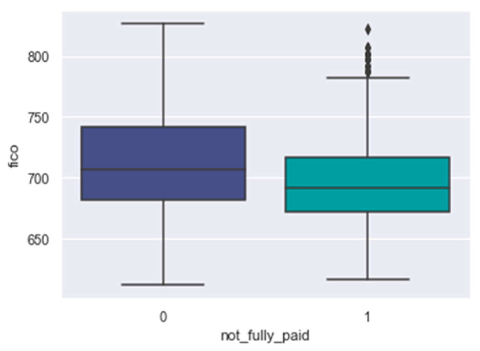
fico: Figure 15 reveals that the FICO scores of defaulters tend to be lower compared to those of borrowers with good repayment records.
Int_rate: Figure 16 showcases that loans not fully paid usually come with higher interest rates when contrasted with fully paid loans.
Inq_last_6mths: Figure 17 shows that defaulters typically have more inquiries during the previous six months. A notable portion (26%) of customers, characterized by having more than 2 inquiries (third quantile of the “inq_last_6mth” attribute) in the last 6 months, eventually become defaulters.
The correlation between the interest rate and FICO scores is depicted for both customer groups (fully paid and not fully paid) presented in Figure 18. The figure demonstrates that individuals with high FICO scores and low interest rates are less prone to default on their loans.
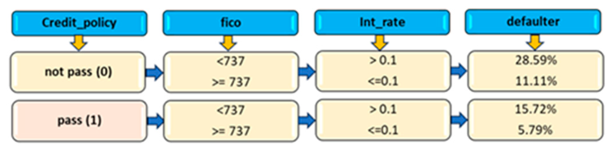
Figure 19 shows borrowers who satisfy or do not satisfy the credit policy criteria, possessing both an interest rate below 0.1 (first quantile of “int_rate”) and a FICO score exceeding 737 (third quantile of “fico”). Remarkably, 6% of borrowers meeting the credit policy criteria end up as loan defaulters. In stark contrast, a considerably higher proportion, amounting to 29%, of clients who do not meet the credit policy criteria, with interest rates surpassing 0.1 and FICO scores falling below 737, fail to repay their loans.
To sum up, our comprehensive data exploration has yielded valuable insights into client behavior. Specifically, loans that end up not being fully paid are typically unable to meet the credit policy, come with extreme interest rates, and have lower FICO scores. These loans also tend to have a higher number of recent inquiries within the last 6 months. Furthermore, when considering the purpose of borrowing, the proportion of defaulters is notably higher in the “small business” category compared to other customer groups.
Moving forward, the insights gained from this exploratory data analysis (EDA) were integrated with a feature selection algorithm to build an effective model for predicting loan defaulters.

4.2. Data Pre-Processing

This process encompasses several steps, including Train Test split, Logarithmic Transformation, Feature Scaling, SMOTE, and Feature Selection. Logarithmic transformation was employed primarily to address skewness in specific numeric attributes closely associated with the class attribute, specifically “instalment”, “fico”, and “day_with_credit_line”. Other attributes do not undergo log transformation as they do not exhibit a log-normal distribution. Notably, Feng et al. [51] have noticed that applying log transformation to right-skewed data can sometimes result in a distribution that is even more skewed than the original one. Figure 20 portrays the distribution of numeric attributes following log transformation. A comparison between Figure 12 and Figure 19 reveals a slight reduction in the skewness of these features.
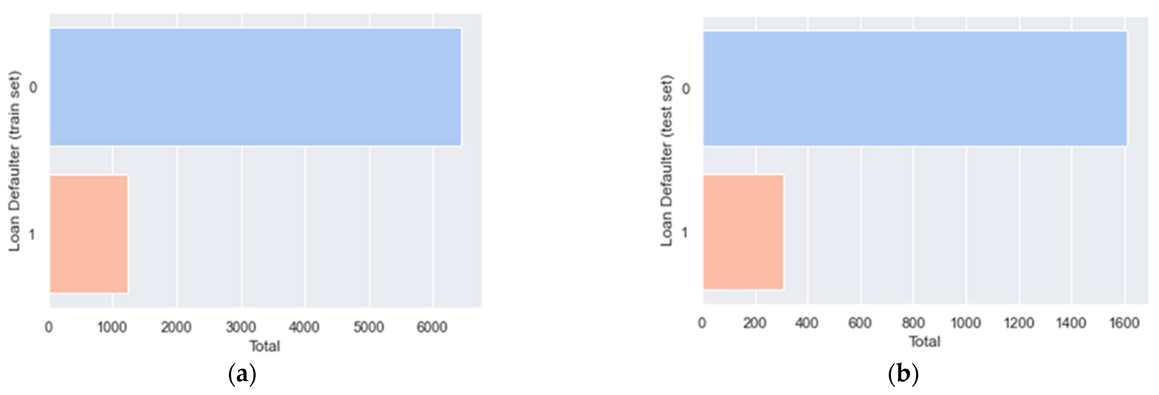
The dataset is divided into training and testing sets, employing a stratified split approach with a test size of 0.2. This ensures that both sets maintain an equal ratio of defaulters and non-defaulters. The respective counts of defaulters and non-defaulters in the training set (a) and testing set (b) are presented in Figure 21.
Given the dataset’s significant class imbalance, where the proportion of defaulters to non-defaulters is roughly 19%, SMOTE is employed to oversample the minority class (defaulters) within the training dataset. This is a crucial step, as utilizing a highly imbalanced dataset could result in machine learning models being biased toward the majority class [32]. Importantly, there is no need to apply SMOTE to the test data to prevent data leakage. Figure 22 illustrates the counts of defaulters (1) and non-defaulters (0) in the training set after SMOTE has been applied.
Feature scaling is a critical step that standardizes all features to the same scale, preventing any single feature from dominating others. If one feature becomes overly dominant, machine learning models may overlook the significance of other features. Standardization, where values are centered around the mean and possess a standard deviation of one, is chosen for feature scaling in this project for its resilience against outliers [13].
For feature selection, Recursive Feature Elimination (RFE) is utilized with Logistic Regression (LR) as the base algorithm. In alignment with the insights from Exploratory Data Analysis (EDA), the decision is made to retain 12 features. As a result of the RFE process, the selected features include credit_policy, encoded purposes, fico, revol_ball, log_annual_income, inq_last_6mths and installment. Interestingly, this outcome aligns with the findings from the EDA. Although a correlation exists between “int_rate” and the “class attribute”, the relatively high correlation coefficient between “fico” and “int_rate” (0.71) may explain why “int_rate” was not selected by RFE.

4.3. Result Achieved by Various ML Algorithms

4.3.1. Logistic Regression

Initially, the machine learning model is trained using Logistic Regression on the training dataset, utilizing the LogisticRegression library from Scikit-Learn [52]. Subsequently, the constructed model is tested, and the outcomes are elaborated upon in Table 3.
The performance of the LR model appears to be relatively modest, yielding an accuracy of 64% and a macro average recall of 62%. The LR correctly predicts 59% of loan defaults, but out of all the loans predicted to be defaulted by the model, only 24% turn out to be defaults, resulting in a precision of 24% for class 1.
To enhance the algorithm’s performance, parameter tuning is conducted, focusing on three parameters: solver, penalty, and C. The GridSearchCV() method is employed to search for the optimal parameter values, which are determined to be ‘C’: 0.01, ‘penalty’: ‘l2’, and ‘solver’: ‘saga’. Subsequently, the model is retrained and tested using these parameter values, and the results are presented in Table 4.
It is evident that parameter tunning did not yield any notable improvement, as the accuracy and recall scores remain at 64% and 62%, respectively.

4.3.2. K-Nearest Neighbors

The KNN algorithm is used to train the ML model on the training dataset, utilizing the KNeighborsClassifier library from Scikit Learn. Subsequently, the constructed model is put to the test, and the outcomes are detailed in Table 5.
The performance of the model appears to be modest, with an accuracy of 67% and a macro average recall of 54%. KNN outperforms LR in identifying good lenders, achieving a recall of 73%, a precision of 85%, and an F1 score of 79%. However, its performance in identifying defaulters is relatively weak.
KNN classifies new data by considering its proximity to neighbors. However, as noted in the exploratory data analysis (EDA), the distribution of the two classes in the target variable is quite similar. This similarity could possibly account for the suboptimal performance [53].
To enhance its performance, parameter tuning is carried out, focusing on three parameters, weight_options, k_range, and metrics. The GridSearchCV() method is employed to search for the best parameter set, resulting in the selection of ‘n_neighbors’: 20, ‘metric’: ‘euclidean’, and ‘weights’: ‘distance’. The model is subsequently retrained and tested using these parameters, and the results are presented (Table 6).
Table 7 and Table 8 reveal a marginal performance improvement, with accuracy increasing from 67% to 69% and recall rising from 54% to 56%.

4.3.3. Support Vector Machine (SVM)

The machine learning model is trained using kernel Support Vector Machine (SVM) on the training dataset, utilizing the SVC library from Scikit-Learn. Subsequently, the constructed model is put to the test, and Table 7 shows the results.
The performance achieved indicates a higher accuracy of 78% compared to KNN and LR. But compared to LR, the recall is less. In addition, SVM struggles to detect defaulters; recall, precision, and f1_score are all below 30%. Nonetheless, SVM excels in predicting non-defaulters, correctly identifying 88% of them.
In addition, parameter tuning is carried out, focusing on three parameters: kernel, C, and gamma. Instead of GridSearchCV(), RandomizedSearchCV() is employed to search for the optimal parameter set, thereby saving time and computational resources. The resulting parameters are ‘C’: 1, ‘gamma’: 1, and ‘kernel’: ‘rbf’. The model is then retrained and tested using kernel SVM, and the results are given in Table 8.
A minor decline in performance is noticeable when compared to Table 8. The drawback of SVM lies in its tuning process, which is notably time- and resource-intensive.

4.3.4. Naïve Bayes

The ML model is trained using NB with the GausianNB library from Scikit learn on the training dataset. Subsequently, the generated model is put to the test, and the outcomes are presented in Table 9.
The performance of the NB model closely resembles that of SVM, achieving an accuracy of 71% and a macro-average recall of 58%. NB excels in predicting good loans, with a precision of 87% for non-defaulters.
To enhance its performance, parameter tuning is conducted. GridSearchCV() is employed to search for the optimal parameter value, resulting in ‘var_smoothing’: 2.848. Subsequently, the model is retrained and tested using this parameter value, and the results are presented in Table 10.
No improvement is observed following parameter tuning, as both the recall and accuracy scores persist at 56% and 71%, respectively.

4.3.5. Decision Tree

The ML model is trained using DT with the DecisionTreeClassifier library from Scikit-Learn on the training dataset. Subsequently, the generated model is put to the test, and the outcomes are presented in Table 11.
The DT algorithm demonstrates enhanced accuracy at 73% in contrast to other algorithms, yet it exhibits lower recall at 53%. Notably, the strength of DT lies in effectively recognizing non-defaulters, achieving a recall of 0.83 and a precision of 85%. However, it demonstrates inefficiency in detecting defaulters, with a recall of 23% and precision of 21%.

4.3.6. Random Forest

The ML model is trained using RF with the RandomForestClassifier library from Scikit-Learn on the training dataset. Subsequently, the generated model is put to the test, and the outcomes are presented in Table 12.
There is a substantial improvement in accuracy compared to other algorithms, reaching 82%. This can be attributed to RF’s capability to amalgamate predictions from various trees to formulate the ultimate prediction for each input. Notably, RF excels in identifying non-defaulters, achieving a recall of 97% and precision of 85%. However, its detection of defaulters is notably deficient, with a recall of 7%.

4.3.7. XGBoost

The XGBoost classifier from the XGBClassifier library is utilized to train the machine learning model. Subsequently, the constructed model undergoes testing, and the outcomes are detailed in Table 13.
The highest accuracy (83%) is achieved in comparison to other algorithms, albeit with a reasonably low recall of 53%. XGBoost also demonstrates strong performance in correctly identifying non-defaulters, with a 97% accuracy rate. However, it struggles to detect defaulters, with a recall of just 9% for class 1.
Parameter tuning was conducted to enhance model performance. Instead of GridSearchCV, RandomizedSearchCV was employed to save time and computational resources. This search resulted in the following optimal parameter values: ‘subsample’: 0.5, ‘‘gamma’: 0.2, objective’: ‘binary:logistic’, ‘min_child_weight’: 5, ‘n_estimators’: 800, ‘max_depth’: 7, and ‘colsample_bytree’: 0.8. The model was subsequently retrained and evaluated using these tuned parameters. However, the results presented in Table 14 indicate that the parameter tuning process did not yield any improvements in model performance.

4.4. Performance Comparison and Analysis

In this section, the performance of various algorithms is assessed to select the most suitable model for our dataset. Subsequently, additional techniques have been implemented to enhance its performance further.
Upon reviewing the confusion matrices and classification reports, it becomes evident that all models exhibit superior performance in the majority class (non-defaulters) compared to the minority class (defaulters). Notably, the tree-based models, such as XGBoost, Decision Trees (DT), and Random Forest (RF), excel in identifying non-defaulters but fall short in accurately identifying defaulters, which is the primary focus of this project.
As previously discussed in Chapter 3 (Section 3.5), given our objective of identifying loan defaulters, the primary metric for assessing the performance of different ML algorithms is recall. Table 15 provides a comparison of recall (macro average) and accuracy for all models, presented as percentages and sorted in descending order of recall values. Notably, LR emerges as the top performer, followed by NB and KNN. LR surpasses other algorithms, including more complex ones like XGBoost and RF, in effectively predicting defaulters. This reaffirms the robustness and applicability of LR in various binary classification scenarios [54]. The systematic experiments conducted in our research work have demonstrated that minimal to no significant improvement was achieved through parameter tuning. Furthermore, in the assessment of algorithmic accuracy, it is observed that XGBoost (XGB) achieves the highest accuracy at 83%, followed by Random Forest (RF) at 82%, and Decision Tree (DT) at 73%.
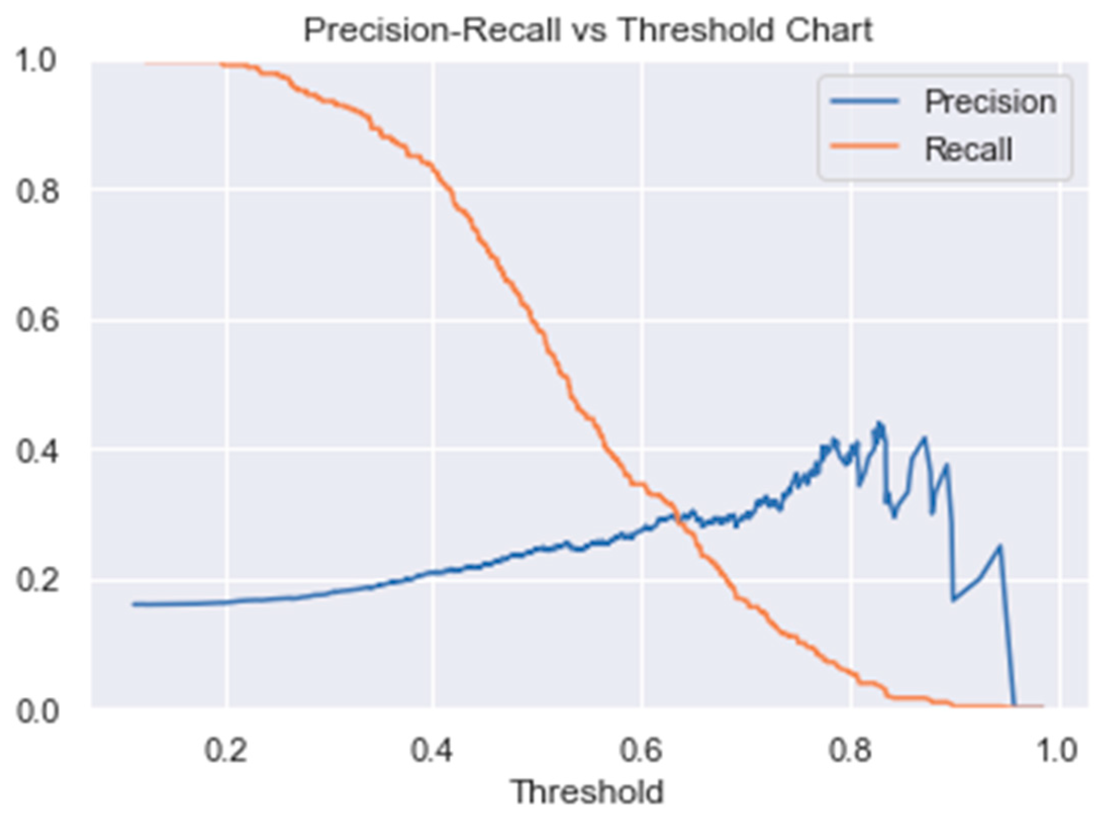
Considering the high recall achieved by LR, potential methods were investigated to enhance its recall for the minority class. Typically, Logistic Regression (LR) categorizes a data point by assessing its probability of being True, utilizing a default threshold set at 0.5. For instance, if the probability surpasses 0.5, the data point is classified as a defaulter; otherwise, it is classified as a non-defaulter. To enhance predictions in class 1 (defaulters), one could consider reducing the decision threshold, especially if it does not significantly impact precision [55]. To explore that, Figure 23 displays recall and precision scores across various threshold values.
Interestingly, it becomes evident that when reducing the threshold, the recall increases at a notably faster rate than precision. For instance, lowering the threshold from 0.5 to 0.4 results in a substantial increase in recall, from 0.58 to 0.83 (an increase of 0.25), while precision experiences only a slight reduction, from 0.24 to 0.21 (a decrease of 0.03).
To delve more profoundly into the analysis, a model is trained and tested with a threshold set at 0.4, employing identical training and testing datasets. The outcomes are outlined in Table 16. It is essential to note that the trade-off between recall and precision implies that by reducing the threshold, there is a risk of rejecting many good customers, as the model may classify them as defaulters and decline their applications. Therefore, it is crucial to exercise caution when considering a significant reduction in the threshold value.

4.5. Critical Analysis of the Study

4.5.1. Strengths of this Proposed Study

By thoroughly exploring data, we pinpoint the financial traits associated with loans that are not repaid. It becomes evident that instances of repayment failure typically involve individuals who do not adhere to the credit policy, carry higher interest rates coupled with lower FICO scores, and exhibit a higher frequency of inquiries in the last 6 months. Furthermore, our analysis has revealed other valuable insights that should be taken into account when making decisions regarding loan applications. These insights include:
  • Customers who borrow funds for small businesses pose a higher risk.
  • The likelihood of a client becoming a defaulter significantly rises when the interest rate exceeds 0.1, and their FICO score falls below 737. Specifically, 28.59% of clients in this category are unlikely to repay their loans, in contrast to a mere 5.79% of clients with interest rates below 0.1 and FICO scores above 737 who are inclined to become loan defaulters.
  • A significant number of individuals who met the credit policy criteria have not fully repaid their loans, indicating a need for the lending institute to review and potentially tighten its credit policy criteria.
In summary, our hypothesis that lenders can predict the likelihood of non-full repayment from clients based solely on their financial information has been validated. ML models were effectively trained for this prediction task. In terms of overall accuracy, XGBoost and RF demonstrated strong performance. However, LR stood out as the top performer for predicting defaulters. LR achieved an 83% correct prediction rate for defaulters with only a minor impact on precision by adjusting its decision threshold to 0.4. Therefore, it is affirmed that lending organizations can derive substantial advantages from utilizing the proposed model as a supportive tool for predicting loan defaulters.

4.5.2. Limitations of the Study

In its present state, the performance of the model slightly falls short of the desired level, as it overlooks the classification of a notable number of loans as defaulters, even though they may actually be repaid. Consequently, it is not recommended for use as an automated loan approval system. Alternatively, it should be utilized to offer additional insights to decision-makers involved in the loan approval process.
The lower accuracy of the model could be attributed to the highly imbalanced dataset, which may cause the models to exhibit a bias towards the majority class, e.g., non-defaulters. Additionally, since the aim is to avoid using personal data, the limited selection of features may have a notable impact on the model’s accuracy.

4.5.3. Comparison with Similar Existing Studies

In comparison to previous ML studies that utilized datasets with a similarly limited number of features (listed in Table 17) and as depicted in Figure 24, our current study demonstrates a significant improvement in the identification of defaulters. The recall, without any threshold adjustments, stands at 0.62, which notably surpasses the recall values of 0.39, 0.45 and 0.19 in previous studies.
By adjusting the decision threshold to 0.4, the recall experiences a substantial improvement, reaching 0.83. Despite our model’s low accuracy when compared to other studies, it is important to note that accuracy is not the most critical metric in this research due to the high degree of imbalance present in all datasets. Additionally, it is worth considering that the primary objective of all aforementioned studies is to identify loan defaults, which represent a relatively rare occurrence when compared to the total number of loans. Hence, prioritizing the reduction of false negatives (instances where loan defaulters are not identified) is considerably more critical than minimizing false positives (identifying non-defaulters as defaulters), given the substantially higher cost associated with false negatives. It is important to highlight that, as this project seeks to refrain from utilizing personal data, the results are not directly comparable to those studies that incorporate personal data, as previously mentioned in the literature review.

5. Conclusions and Future Research Directions

Predicting the occurrence of loan defaults has shown to be difficult yet crucial for successful and sustainable development in the P2P lending industry as well as other financial sectors. To further minimize losses, it is crucial to identify high-risk clients during the loan application process. An effective computational model for determining whether a loan is likely to be repaid has been developed in this project using a machine learning (ML) approach. The goal is to support lenders in their decision-making by doing so.
According to the findings of careful data exploration research, borrowers who do not adhere to the lending institution’s credit policy, pay higher interest rates and have lower FICO scores are more likely to default. Customers who obtained a small business loan also showed signs of high risk. Additionally, it has been observed that they tended to make more inquiries in the previous six months. Overall, our data exploration findings offer significant and practical insights into client behavior that could help lenders make better loan decisions.
In the pursuit of refining a model capable of distinguishing borrowers likely to repay their loans from those who are not, we have explored prominent machine learning classification algorithms, including Support Vector Machine, Logistic Regression, Decision Tree, XGBoost, Naïve Bayes, and Random Forest.
These algorithms were chosen based on the results of our data exploration. The best accuracy was attained by XGBoost and Random Forest, topping 80%. Setting the decision threshold at 0.5 (the default threshold of Logistic Regression) and 0.4 (with minimal impact on the precision score) accurately identifies 62% and 83% of defaulted loans, respectively. This is the best performance for predicting loan defaulters. Overall, our findings provided useful insights into borrowers’ behavioral patterns and how to use ML classification algorithms to improve lending decision-making. In real-world lending scenarios, the model can be employed to offer additional insights to decision-makers when approving loans.
Comparing this performance to earlier ML research that used datasets with fewer features is impressive (again, see Table 17). This discovery suggests that we might be able to accurately anticipate loan defaulters without profoundly depending on data containing personal information (which might raise numerous ethical and security issues) [57]. New data can be gathered in future work with new features to enhance classification performance. Finding a healthy balance about whether personal data is most crucial and unavoidable for obtaining great performance may be necessary if the goal is to continue avoiding overly depending on personal data. In addition, more sophisticated feature selection methods like LDA and PCA can be investigated to enhance the performance of the models. Finally, we intend to investigate other cutting-edge ML algorithms, including alternative ANN topologies and deep learning algorithms.

Author Contributions

All authors had an equal contribution in preparing and finalizing the manuscript. Conceptualization: L.N. and M.A.; methodology, L.N. and M.A.; validation: L.N., M.A. and J.H.; formal analysis: L.N., M.A. and J.H.; investigation: L.N., M.A. and J.H.; data curation: L.N., writing—original draft preparation: L.N. and M.A.; writing—review and editing: L.N., M.A. and J.H.; supervision: M.A. and J.H. All authors have read and agreed to the published version of the manuscript.

Funding

This research received no external funding.

Institutional Review Board Statement

Not applicable.

Informed Consent Statement

Not applicable.

Data Availability Statement

Data are contained within the article.

Acknowledgments

It is acknowledged that part of this research work was taken from an MSc project report submitted to the University of York. An AI tool was employed to improve the English language in some places.

Conflicts of Interest

Author Ly Nguyen was employed by Emissis Ltd. The authors declare no conflicts of interest.

References

  1. Nowak, A.; Ross, A.; Yencha, C. Small business borrowing and peer-to-peer lending: Evidence from lending club. Contemp. Econ. Policy 2018, 36, 318–336. [Google Scholar] [CrossRef]
  2. Jiang, C.; Wang, Z.; Wang, R.; Ding, Y. Loan default prediction by combining soft information extracted from descriptive text in online peer-to-peer lending. Ann. Oper. Res. 2018, 266, 511–529. [Google Scholar] [CrossRef]
  3. Gerhard, F.; Harlalka, A.; Kremer, A.; Suvanam, R. The Coming Opportunity in Consumer Lending; McKinsey & Company: Berlin, Germany, 2021. [Google Scholar]
  4. Kun, Z.; Feng, W.; Wu, J. Default Identification of P2P Lending Based on Stacking Ensemble Learning. In Proceedings of the 2020 2nd International Conference on Economic Management and Model Engineering (ICEMME), Chongqing, China, 20–22 November 2020; pp. 992–1006. [Google Scholar]
  5. Xu, J.; Lu, Z.; Xie, Y. Loan default prediction of Chinese P2P market: A machine learning methodology. Sci. Rep. 2021, 11, 18759. [Google Scholar] [CrossRef]
  6. Rai, H.M.; Yoo, J. Analysis of Colorectal and Gastric Cancer Classification: A Mathematical Insight Utilizing Traditional Machine Learning Classifiers. Mathematics 2023, 11, 4937. [Google Scholar] [CrossRef]
  7. Freedman, S.; Jin, G.Z. Do Social Networks Solve Information Problems for Peer-to-Peer Lending? Evidence from Prosper.com. NET Institute Working Paper No. 08-43, Indiana University, Bloomington: School of Public & Environmental Affairs Research Paper No. 2008-11-06. Available online: https://ssrn.com/abstract=1936057 (accessed on 14 November 2008).
  8. Pope, D.G.; Sydnor, J.R. What’s in a Picture? Evidence of Discrimination from Prosper. com. J. Hum. Resour. 2011, 46, 53–92. [Google Scholar]
  9. Chen, X.; Ding, X.; Wang, B. A study of the overdue behaviors in private borrowing—Empirical analysis based on P2P network borrowing and lending. Proc. Financ. Forum 2013, 11, 10. [Google Scholar]
  10. Agrawal, A.; Gans, J.; Goldfarb, A. Prediction Machines: The Simple Economics of Artificial Intelligence; Harvard Business Press: Boston, MA, USA, 2018. [Google Scholar]
  11. Bessis, J. Risk Management in Banking; John Wiley & Sons: Hoboken, NJ, USA, 2011. [Google Scholar]
  12. Tan, P.-N.; Steinbach, M.; Kumar, V. Introduction to Data Mining; Pearson Education India: Delhi, India, 2016. [Google Scholar]
  13. Ruyu, B.; Mo, H.; Haifeng, L. A Comparison of Credit Rating Classification Models Based on Spark-Evidence from Lending-club. Procedia Comput. Sci. 2019, 162, 811–818. [Google Scholar] [CrossRef]
  14. Zhu, L.; Qiu, D.; Ergu, D.; Ying, C.; Liu, K. A study on predicting loan default based on the random forest algorithm. Procedia Comput. Sci. 2019, 162, 503–513. [Google Scholar] [CrossRef]
  15. Kumar, V.; Natarajan, S.; Keerthana, S.; Chinmayi, K.; Lakshmi, N. Credit risk analysis in peer-to-peer lending system. In Proceedings of the 2016 IEEE International Conference on Knowledge Engineering and Applications (ICKEA), Singapore, 28–30 September 2016; pp. 193–196. [Google Scholar]
  16. Maheswari, P.; Narayana, C.V. Predictions of Loan Defaulter-A Data Science Perspective. In Proceedings of the 2020 5th International Conference on Computing, Communication and Security (ICCCS), Patna, India, 14–16 October 2020; pp. 1–4. [Google Scholar]
  17. Juneja, S. Defaulter Prediction for Assessment of Credit Risks using Machine Learning Algorithms. In Proceedings of the 2020 4th International Conference on Electronics, Communication and Aerospace Technology (ICECA), Coimbatore, India, 5–7 November 2020; pp. 1139–1144. [Google Scholar]
  18. Malekipirbazari, M.; Aksakalli, V. Risk assessment in social lending via random forests. Expert Syst. Appl. 2015, 42, 4621–4631. [Google Scholar] [CrossRef]
  19. Xia, Y.; Liu, C.; Liu, N. Cost-sensitive boosted tree for loan evaluation in peer-to-peer lending. Electron. Commer. Res. Appl. 2019, 24, 30–49. [Google Scholar] [CrossRef]
  20. Emekter, R.; Tu, Y.; Jirasakuldech, B.; Lu, M. Evaluating credit risk and loan performance in online Peer-to-Peer (P2P) lending. Appl. Econ. 2015, 47, 54–70. [Google Scholar] [CrossRef]
  21. Jin, Y.; Zhu, Y. A data-driven approach to predict default risk of loan for online peer-to-peer (P2P) lending. In Proceedings of the 2015 Fifth International Conference on Communication Systems and Network Technologies, Gwalior, India, 4–6 April 2015. [Google Scholar]
  22. Kamiri, J.; Mariga, G. Research Methods in Machine Learning: A Content Analysis. Int. J. Comput. Inf. Technol. 2021, 10, 78–91. [Google Scholar] [CrossRef]
  23. Harvard University. Harvard Dataverse Repository. Available online: https://dataverse.harvard.edu/ (accessed on 23 April 2023).
  24. University of California Irvine. UCI Machine Learning Repository. Available online: https://archive.ics.uci.edu/ml/datasets/credit+approval (accessed on 20 February 2023).
  25. Chu, X.; Ilyas, I.F.; Krishnan, S.; Wang, J. Data cleaning: Overview and emerging challenges. In Proceedings of the 2016 International Conference on Management Of Data, San Francisco, CA, USA, 26 June–1 July 2016; pp. 2201–2206. [Google Scholar]
  26. Diez, D.M.; Barr, C.D.; Cetinkaya-Rundel, M. OpenIntro Statistics; OpenIntro: Boston, MA, USA, 2012; pp. 174–175. [Google Scholar]
  27. Kelleher, J.D.; Tierney, B. Data Science; MIT Press: Cambridge, MA, USA, 2018. [Google Scholar]
  28. Jakulin, A. Machine Learning Based on Attribute Interactions. Ph.D. Thesis, Univerza v Ljubljani, Ljubljana, Slovenia, 2005. [Google Scholar]
  29. Cerda, P.; Varoquaux, G.; Kégl, B. Similarity encoding for learning with dirty categorical variables. Mach. Learn. 2018, 107, 1477–1494. [Google Scholar] [CrossRef]
  30. Alshaher, H. Studying the Effects of Feature Scaling in Machine Learning. Ph.D. Thesis, North Carolina Agricultural and Technical State University, Greensboro, NC, USA, 2021. [Google Scholar]
  31. Zheng, A.; Casari, A. Feature Engineering for Machine Learning: Principles and Techniques for Data Scientists; O’Reilly Media, Inc.: Sebastopol, CA, USA, 2018. [Google Scholar]
  32. Gosain, A.; Sardana, S. Handling class imbalance problem using oversampling techniques: A review. In Proceedings of the 2017 International Conference on Advances in Computing, Communications and Informatics (ICACCI), Udupi, India, 13–16 September 2017; pp. 79–85. [Google Scholar]
  33. Mohammed, R.; Rawashdeh, J.; Abdullah, M. Machine learning with oversampling and undersampling techniques: Overview study and experimental results. In Proceedings of the 2020 11th International Conference on Information and Communication Systems (ICICS), Irbid, Jordan, 7–9 April 2020; pp. 243–248. [Google Scholar]
  34. Haibo, H.; Yunqian, M. Imbalanced Learning: Foundations, Algorithms, and Applications; Wiley-IEEE Press: New York, NY, USA, 2013; Volume 1, p. 27. [Google Scholar]
  35. Chawla, N.V. Data mining for imbalanced datasets: An overview. In Data Mining and Knowledge Discovery Handbook; Springer: Boston, MA, USA, 2009; pp. 875–886. [Google Scholar] [CrossRef]
  36. Sánchez-Maroño, N.; Alonso-Betanzos, A.; Tombilla-Sanromán, M. Filter methods for feature selection—A comparative study. In Proceedings of the International Conference on Intelligent Data Engineering and Automated Learning, Birmingham, UK, 16–19 December 2007; pp. 178–187. [Google Scholar]
  37. Yan, K.; Zhang, D. Feature selection and analysis on correlated gas sensor data with recursive feature elimination. Sens. Actuators B Chem. 2015, 212, 353–363. [Google Scholar] [CrossRef]
  38. Tu, J.V. Advantages and disadvantages of using artificial neural networks versus logistic regression for predicting medical outcomes. J. Clin. Epidemiol. 1996, 49, 1225–1231. [Google Scholar] [CrossRef] [PubMed]
  39. Jadhav, S.D.; Channe, H. Comparative study of K-NN, naive Bayes and decision tree classification techniques. Int. J. Sci. Res. IJSR 2016, 5, 1842–1845. [Google Scholar]
  40. Yeh, I.-C.; Lien, C. The comparisons of data mining techniques for the predictive accuracy of probability of default of credit card clients. Expert Syst. Appl. 2009, 36, 2473–2480. [Google Scholar] [CrossRef]
  41. Cortes, C.; Vapnik, V. Support-vector networks. Mach. Learn. 1995, 20, 273–297. [Google Scholar] [CrossRef]
  42. Sharma, H.; Kumar, S. A survey on decision tree algorithms of classification in data mining. Int. J. Sci. Res. IJSR 2016, 5, 2094–2097. [Google Scholar]
  43. Ma, X.; Sha, J.; Wang, D.; Yu, Y.; Yang, Q.; Niu, X. Study on a prediction of P2P network loan default based on the machine learning LightGBM and XGboost algorithms according to different high dimensional data cleaning. Electron. Commer. Res. Appl. 2018, 31, 24–39. [Google Scholar] [CrossRef]
  44. McKinney, W. Python for Data Analysis: Data Wrangling with Pandas, NumPy, and IPython; O’Reilly Media, Inc.: Newton, MA, USA, 2012. [Google Scholar]
  45. Raschka, S.; Mirjalili, V. Python Machine Learning: Machine Learning and Deep Learning with Python, Scikit-Learn, and TensorFlow 2; Packt Publishing Ltd.: Birmingham, UK, 2019. [Google Scholar]
  46. Reitermanova, Z. Data splitting. In WDS; Matfyzpress: Prague, Czech Republic, 2010; Volume 10, pp. 31–36. [Google Scholar]
  47. May, R.J.; Maier, H.R.; Dandy, G.C. Data splitting for artificial neural networks using SOM-based stratified sampling. Neural Netw. 2010, 23, 283–294. [Google Scholar] [CrossRef] [PubMed]
  48. Yang, L.; Shami, A. On hyperparameter optimization of machine learning algorithms: Theory and practice. Neurocomputing 2020, 415, 295–316. [Google Scholar] [CrossRef]
  49. Ranjan, G.; Verma, A.K.; Radhika, S. K-nearest neighbors and grid search cv based real time fault monitoring system for industries. In Proceedings of the 2019 IEEE 5th International Conference for Convergence in Technology (I2CT), Bombay, India, 29–31 March 2019; pp. 1–5. [Google Scholar]
  50. Agrawal, T. Hyperparameter optimization using scikit-learn. In Hyperparameter Optimization in Machine Learning; Springer: Berlin/Heidelberg, Germany, 2021; pp. 31–51. [Google Scholar]
  51. Feng, C.; Wang, H.; Lu, N.; Chen, T.; He, H.; Lu, Y. Log-transformation and its implications for data analysis. Shanghai Arch. Psychiatry 2014, 26, 105. [Google Scholar] [PubMed]
  52. Asar, Y. Some new methods to solve multicollinearity in logistic regression. Commun. Stat.-Simul. Comput. 2017, 46, 2576–2586. [Google Scholar] [CrossRef]
  53. Abu Alfeilat, H.A.; Hassanat, A.B.; Lasassmeh, O.; Tarawneh, A.S.; Alhasanat, M.B.; Eyal Salman, H.S.; Prasath, V.S. Effects of distance measure choice on k-nearest neighbor classifier performance: A review. Big Data 2019, 7, 221–248. [Google Scholar] [CrossRef] [PubMed]
  54. Maalouf, M. Logistic regression in data analysis: An overview. Int. J. Data Anal. Tech. Strateg. 2011, 3, 281–299. [Google Scholar] [CrossRef]
  55. Handoyo, S.; Chen, Y.-P.; Irianto, G.; Widodo, A. The Varying Threshold Values of Logistic Regression and Linear Discriminant for Classifying Fraudulent Firm. Math. Stat. 2021, 9, 135–143. [Google Scholar] [CrossRef]
  56. Silva, E.C.E.; Lopes, I.C.; Correia, A.; Faria, S. A logistic regression model for consumer default risk. J. Appl. Stat. 2020, 47, 2879–2894. [Google Scholar] [CrossRef]
  57. Hu, B.; Zhang, Z.; Zhou, J.; Fang, J.; Jia, Q.; Fang, Y.; Yu, Q.; Qi, Y. Loan default analysis with multiplex graph learning. In Proceedings of the 29th ACM International Conference on Information & Knowledge Management, Virtual, 19–23 October 2020; pp. 2525–2532. [Google Scholar]
Figure 1. Overall research design of the proposed work, from Data Collection (Section 3.1.) to Data Exploration (Section 3.2), Data Pre-Processing (Section 3.3.), Computational Method (Section 3.4.), Model Training and Testing (Section 3.5) and finally, Results and Evaluation (Section 4).
Fintech 03 00012 g001
Figure 2. The S-curve represents the Sigmoid function in logistic regression.
Fintech 03 00012 g002
Figure 3. Categorize a new data point using the K-Nearest Neighbors (KNN) algorithm: before KNN (on the left) and after KNN (on the right).
Fintech 03 00012 g003
Figure 4. Data classification using the SVM algorithm.
Fintech 03 00012 g004
Figure 5. The configuration of a decision tree.
Fintech 03 00012 g005
Figure 6. The configuration of a Random Forest.
Fintech 03 00012 g006
Figure 7. Visualization of the XGBoost algorithm.
Fintech 03 00012 g007
Figure 8. Information regarding attribute types and the presence of missing data.
Fintech 03 00012 g008
Figure 9. Number of loans categorized by their borrowing purposes.
Fintech 03 00012 g009
Figure 10. The percentage of loans that are not fully paid and fully paid categorized by the purpose of borrowing.
Fintech 03 00012 g010
Figure 11. Correlation among numeric variables.
Fintech 03 00012 g011
Figure 12. Comparison of correlations with the class attribute.
Fintech 03 00012 g012
Figure 13. Histogram depicting the distribution of numeric variables.
Fintech 03 00012 g013
Figure 14. Client counts categorized by credit criteria (a), along with the percentage of fully paid and not fully paid clients within each credit policy category (b).
Fintech 03 00012 g014
Figure 15. A box plot depicting FICO scores for borrowers categorized as fully paid and not fully paid.
Fintech 03 00012 g015
Figure 16. A box plot depicting the interest rates for borrowers categorized as fully paid and not fully paid.
Fintech 03 00012 g016
Figure 17. Box plot representing the attribute “inq_last_6mths” for fully paid and not fully paid borrowers.
Fintech 03 00012 g017
Figure 18. Scatterplot of interest rate and fico scores, categorized by loan payment status.
Fintech 03 00012 g018
Figure 19. The relationship between credit policy, interest rate, FICO and the class attribute.
Fintech 03 00012 g019
Figure 20. Histograms depict the distribution of numeric attributes after log transformation.
Fintech 03 00012 g020
Figure 21. The total of defaulters and non-defaulters in the training set (a) and testing set (b) following the train test split.
Fintech 03 00012 g021
Figure 22. Number of defaulters (1) and non-defaulters (0) following SMOTE.
Fintech 03 00012 g022
Figure 23. Graphs illustrating precision and recall scores across different threshold values.
Fintech 03 00012 g023
Figure 24. Performances Comparison between existing works (Juneja [17] and Costa e Silva, et al [26]) and the proposed approach.
Fintech 03 00012 g024
Table 1. Sample of raw loan dataset.
credit.policyPurposeint.rateinstallmentlog.annual.incdtificodays.with.cr.linerevol.ballrevol.utilinq.last.6mthsdelinq.2yrspub.recnot.fully.paid
1debt_consolidation0.1189829.111.3504065419.487375639.95828,85452.10000
1credit_card0.1071228.2211.0821425514.29707276033,62376.70000
1debt_consolidation0.1357366.8611.3504065411.636824710351125.61000
1debt_consolidation0.1008162.3411.299732248.17122699.95833,66773.21000
1credit_card0.1426102.9211.9049675514.976674066474039.50100
1credit_card0.0788125.1310.7144177716.98727612050,807510000
1debt_consolidation0.1496194.0211.0020998446673180383976.80011
1all_other0.1114131.2211.4075649511.08722511624,22068.60001
Table 2. Attribute information overview.
IndexAttributesType of
Attribute
Number of Unique ValuesAttribute Details
0credit.policyNumerical21 if the client meets the credit policy of Lending Club, 0 otherwise.
1purposeCategorical7The purpose of the loan (values: “credit_card”, “debt_consolidation”, “educational”, “major_purchase”, ‘home_improvement” “small_business”, and “all_other”).
2int.rateNumerical249The interest rate of the loan (a rate of 9% is stored as 0.09).
3instalmentNumerical4788The monthly installments owned by the borrower if the loan is funded.
4log.annual.incNumerical1987The natural log of the annual income of the borrower.
5dtiNumerical2529The debt-to-income ratio of the borrower.
6ficoNumerical44The FICO credit score of the borrower.
7days.with.cr.lineNumerical2687The number of days the borrower has had a credit line.
8revol.ballNumerical7869The borrower’s revolving balance (amount unpaid at the end of the credit card billing cycle).
9revol.utilNumerical1035The borrower’s revolving line utilization rate (the amount of the credit line used relative to total credit available).
10inq.last.6mthsNumerical28The borrower’s number of inquiries by creditors in the last 6 months.
11delinq.2yrsNumerical11The number of times the borrower had been 30+ days past due on a payment in the past 2 years.
12pub.recNumerical6The borrower’s number of derogatory public records.
13not.fully.paidNumerical21 if the loan is not fully paid, 0 otherwise.
Table 3. Classification report obtained from the LR model.
PrecisionRecallF1 ScoreSupport
Non-defaulter89%65%75%1609
Defaulter24%59%34%307
Accuracy 64%1916
Macro average57%62%55%1916
Weighted average79%64%68%1916
Table 4. Classification report obtained from the LR model after parameter tuning.
PrecisionRecallF1 ScoreSupport
Non-defaulter89%66%76%1609
Defaulter24%59%34%307
Accuracy 64%1916
Macro average57%62%55%1916
Weighted average79%64%69%1916
Table 5. Classification report obtained from the KNN model.
PrecisionRecallF1 ScoreSupport
Non-defaulter85%73%79%1609
Defaulter20%34%25%307
Accuracy 67%1916
Macro average52%54%52%1916
Weighted average75%67%70%1916
Table 6. Classification report obtained from the KNN model after parameter tuning.
PrecisionRecallF1 ScoreSupport
Non-defaulter86%75%80%1609
Defaulter22%36%27%307
Accuracy 69%1916
Macro average54%56%54%1916
Weighted average76%69%72%1916
Table 7. Classification report obtained from the SVM model.
PrecisionRecallF1 ScoreSupport
Non-defaulter86%88%87%1609
Defaulter28%24%26%307
Accuracy 78%1916
Macro average57%56%56%1916
Weighted average77%78%77%1916
Table 8. Classification Report obtained from the SVM model after parameter tuning.
PrecisionRecallF1 ScoreSupport
Non-defaulter85%88%87%1609
Defaulter23%19%21%307
Accuracy 77%1916
Macro average54%54%54%1916
Weighted average75%77%76%1916
Table 9. Classification report obtained from the NB algorithm.
PrecisionRecallF1 ScoreSupport
Non-defaulter87%77%81%1609
Defaulter24%39%30%307
Accuracy 71%1916
Macro average56%58%56%1916
Weighted average77%71%73%1916
Table 10. Classification report obtained from the NB algorithm after parameter tuning.
PrecisionRecallF1 ScoreSupport
Non-defaulter87%77%81%1609
Defaulter24%39%30%307
Accuracy 71%1916
Macro average57%62%55%1916
Weighted average79%64%68%1916
Table 11. Classification report obtained from the DT classifier.
PrecisionRecallF1 ScoreSupport
Non-defaulter85%83%84%1609
Defaulter21%23%22%307
Accuracy 73%1916
Macro average53%53%53%1916
Weighted average75%73%74%1916
Table 12. Classification report obtained from the RF algorithm.
PrecisionRecallF1 ScoreSupport
Non-defaulter85%97%90%1609
Defaulter30%7%12%307
Accuracy 82%1916
Macro average57%52%51%1916
Weighted average76%82%78%1916
Table 13. Classification report obtained from the XGBoost classifier.
PrecisionRecallF1 ScoreSupport
Non-defaulter 85%97%91%1609
Defaulter36%9%14%307
Accuracy 83%1916
Macro average61%53%52%1916
Weighted average77%83%78%1916
Table 14. Classification report obtained from the XGBoost after parameter tuning.
PrecisionRecallF1 ScoreSupport
Non-defaulter85%90%87%1609
Defaulter21%14%16%307
Accuracy 78%1916
Macro average53%52%52%1916
Weighted average74%78%76%1916
Table 15. Evaluating and comparing the recall and accuracy metrics across all models.
ModelRecall (%)Accuracy (%)
Logistic Regression6264
Logistic Regression parameter tunning6264
Naïve Bayes5871
Naïve Bayes parameter tunning5871
SVM5678
KNN parameter tunning5669
KNN5467
SVM parameter tunning5477
XGBoost5383
Random Forest5282
XGBoost parameter tunning5278
Decision Tree5173
Table 16. Classification report obtained from LR model with a threshold equal to 0.4.
PrecisionRecallF1 ScoreSupport
00.920.400.561609
10.210.830.33307
Accuracy 0.471916
Macro average0.570.610.451916
Weighted average0.810.470.521916
Table 17. Performance comparisons between existing similar works and the proposed research work.
StudyDatasetML AlgorithmRecallAccuracy
Juneja [17]dataset 1:
attributes: 13
LR45%80%
Juneja [17]dataset 2:
attributes: 25
LR39%80%
Costa e Silva, Eliana, et al. [56]14 attributesLR19%90%
The proposed study
(Without adjusting threshold)
14 attributesLR62%64%
Disclaimer/Publisher’s Note: The statements, opinions and data contained in all publications are solely those of the individual author(s) and contributor(s) and not of MDPI and/or the editor(s). MDPI and/or the editor(s) disclaim responsibility for any injury to people or property resulting from any ideas, methods, instructions or products referred to in the content.

