Regulated LSTM Artificial Neural Networks for Option Risks

Abstract

This research aims to study the pricing risks of options by using improved LSTM artificial neural network models and make direct comparisons with the Black–Scholes option pricing model based upon the option prices of 50 ETFs of the Shanghai Securities Exchange from 1 January 2018 to 31 December 2019. We study an LSTM model, a mathematical option pricing model (BS model), and an improved artificial neural network model—the regulated LSTM model. The method we adopted is first to price the options using the mathematical model—i.e., the BS model—and then to construct the LSTM neural network for training and predicting the option prices. We further form the regulated LSTM network with optimally selected key technical indicators using Python programming aiming at improving the network’s predicting ability. Risks of option pricing are measured by MSE, RMSE, MAE and MAPE, respectively, for all the models used. The results of this paper show that both the ordinary LSTM and the traditional BS option pricing model have lower predictive ability than the regulated LSTM model. The prediction ability of the regulated LSTM model with the optimal technical indicators is superior, and the approach adopted is effective.

1. Introduction

With the rapid development of international financial markets, financial derivatives, such as forward contracts, futures and options, have been developed to a great extent. In as early as 1900, Loures Bachelier published an article on option pricing [1]. However, this contribution did not receive a wide recognition. Since the 1970s, with the rapid growth of the derivative market, the research on option pricing theory had made remarkable breakthroughs. For instance, Fischer Black and Myron Scholes [2] proposed the very first complete option pricing model, which was also known as Black–Scholes model (or B-S model), and won the Nobel Prize in Economics in 1990. Thereafter, an enormous amount of research work was conducted in relation to the B-S model. Notably, Benaroch and Kauffman [3] used the Black–Scholes model to study the deployment of POS point debit services. Kou [4] optimized the B-S model and proposed the jump-diffusion model, which can provide analytical solutions for various options pricing problems, including call and put options and interest rate derivatives. Along with this line of research, many other option models have been developed by researchers. For example, Carr and Wu [5] studied time-changed Levy process and used the eigenfunction technique to directly select and test a specific option pricing model; their framework included almost all the models proposed in the option pricing literature. Because of the invention of the Black–Scholes model, option pricing has attracted a strong wave of enthusiasm, and this model has been widely used as a milestone in many areas.

In recent years, artificial intelligence (AI) applications such as such as neural networks have provided exciting algorithms for option risks. Unlike mathematical option models, the complex relationship between inputs and outputs can be established via machine learning without a need to consider the economic principles. For examples, Yao, Li and Tan [6] use the Multilayer Perceptron (MLP) network (i.e., the Error Back Propagation multilayer algorithm) to predict the futures option prices of the Nikkei 225 Index. Their results show that the neural network option pricing model performs better than the traditional Black–Scholes model in the fluctuating market. In addition, similar conclusions were obtained by Lin and Yeh [7]. They used the B-P neural network and the Black–Scholes pricing model to predict option prices of the Taiwan stock index. Their data include the daily price of the sample option during the period from 2 January 2002 to 31 December 2003. The empirical evidence shows that the neural network option pricing model outperforms the traditional Black–Scholes model in the volatile market. More related research work can be found elsewhere [8,9,10].

Thanks to the rapid development of AI and machine learning, new types of artificial neural networks have been proposed; for example, in 1997, Sepp Hochreiter and Jurgen Schmidhuber [11] proposed the neural network of long short-term memory (LSTM). Because LSTM neural networks use “gates” to control the memory process, they can solve some problems that require a long time span. On the basis of the LSTM model, Graves and Schmidhuber [12] proposed bidirectional long short-term memory neural network (BLSTM), which is the most widely used LSTM model so far. Xie and You [13] have applied LSTM neural networks in finance. They believe that LSTMs have a superiority for the pricing of financial derivatives. Fischer and Krauss [14] reported the performance of LSTM models in predicting financial markets using S&P 500 data from 1992 to 2015 and demonstrated that LSTM models outperform traditional machine learning methods.

There has been extensive study regarding the significance and usefulness of technical indicators (TIs) in finance. For instance, Zhu and Pan [15] show that the Money Flow Index (MFI) can accurately predict the price of Chinese stocks. Ko et al. [16] established that by applying a moving average time strategy to a portfolio structured in accordance with a book-to-market ratio, a higher rate of return can be generated than with a buy-and-hold strategy in the Taiwan stock market. Nelson, Pereira and de Oliveira [17] presented a model for predicting stock price movement based on LSTM. Using auto encoder and kernel extreme learning machine, the deep learning models can enhance the quality of forecasts for financial market (Mohanty, Parida and Khuntia [18]). Notably, LSTM with technical and macroeconomic indicators has recently been used for forecasting directional movement of Forex market [19] and for stock price movement [20].

So far, the LSTM neural networks combined with technical indicators have not been exploited adequately for option risks, which is the primary aim of this research. Furthermore, technical indicators have not been selected optimally in the previous research. The contributions of this study are as follows:

• A popular deep learning tool called LSTM, which is frequently used to forecast values in time-series data, is adopted to predict SSE50 ETF option prices.
• Instead of TIs “farming”, key technical indicators are optimally identified using two statistical methods for financial options: F-Regression and Mutual Information Regression. This idea improves the situation in which technical indicators are often included without considering their weights of contributions to forecasted results.
• A novel regulated LSTM model is proposed for option risks that combines the two different approaches with decision rules to increase pricing accuracy.
• The proposed model models are tested using real data (SSE50 ETF options) to demonstrate that the regulated LSTM model outperforms others.

Next, we will present our preliminary research outcomes on the pricing performance of LSTM on financial options. We will compare the pricing accuracy of the Nobel-winning BS model, the traditional LSTM, and the regulated LSTM model with incorporated technical indicators.

2. Models

2.1. B-S Model

As a major milestone achievement, Fischer Black and Myron Scholes [21] proposed the first integrated theory of option pricing in 1973, which is an important contribution to the theory of option pricing. There is a vast body of literature on option pricing with “advanced” methods with an aim to improve the B-S model, such as stochastic volatility models [22,23]; models with jump-diffusion process [24], in which the jump components of asset price follow the compound Poisson process; and more general Levy processes [25,26], which allow the jump components to have infinite activity and admits nearly an arbitrary distribution. However, these models are more suitable for pricing stock options where the stock price (i.e., the underlying) tends to exhibit a significant volatile feature (such as frequent large jumps). As discussed in our recent research [27], complex models that involve sophisticated features in the time series such as regime-switching in the underlying asset may not always offer advantages over traditional models for option pricing in consideration of model uncertainty and the computation effort involved. As such, we have opted for the conventional B-S model based on the following rationales. (1) The underlying asset for the options we have studied is the SSE 50 ETF [28], which is an Exchange Traded Fund that is composed of China 50 Exchange Traded Open-End Index Securities. The SSE 50 Index consists of 50 leading companies from industries in different sectors as “blue chips”; therefore, the resulting SSE 50 ETF is much less volatile than an individual stock, which provides reasonable conditions for the BS-model assumptions such as “Efficient Market” and constant volatility. (2) The length of maturity for the options on the SSE 50 ETF we have considered is less than 1 year (most maturities of the options studied are between 3 months and 6 months), which makes the B-S model more suitable as a “reference” model in our case. In addition, we use GARCH (1,1) to generate dynamic market volatilities, replacing the traditional way of estimating historical volatility.

In our study, the price of the underlying asset fluctuates randomly and follows geometric Brownian motion:

$$dS=\mu Sdt+\sigma Sdz$$

(1)

where S is the price of the underlying asset; μ is the expected annual yield; t is time; σ is the volatility of the underlying asset price; dz is the wiener process; and the price of the underlying asset uses the ITO lemma,

$$df=\left(\frac{\partial f}{\partial S}\mu S+\frac{\partial f}{\partial t}+\frac{1}{2}\frac{{\partial }^{2}f}{\partial S^2}{\sigma }^2{S}^2\right)dt+\frac{\partial f}{\partial S}\sigma Sdz$$

(2)

The Black–Scholes European option pricing equation is shown as follows:

$$\frac{\partial f}{\partial t}+rS\frac{\partial f}{\partial S}+\frac{1}{2}{\sigma }^2{S}^2\frac{{\partial }^{2}f}{\partial S^2}=rf$$

(3)

It can be concluded from the analysis that μ is related to investors’ risk preference. The more risk-averse an investor is, the higher μ will be for any stock. From the B-S differential equation, it can be seen that the expected annual return μ does not appear in the equation, so investors’ arbitrary risk preference will not affect the solution of the equation. Consequently, this equation is risk neutral.

2.1.1. Volatility

Volatility is considered as an important factor for the option risks. In our study, the maximum likelihood method is used to estimate the parameters ω, α, β in GARCH (1,1). The formula of GARCH (1,1) used is given below:

$${\sigma }_i^2=\omega +\alpha ·{\sigma }_{i-1}^2+\beta ·r_{i-1}^2$$

(4)

Define $v_i={\sigma }_i^2$ as the estimation of the variance for the ith day. The likelihood function is:

$${\displaystyle \sum }_{i=1}^m\left[-ln\left(v_i\right)-\frac{u_i^2}{v_i}\right]$$

(5)

where

$$u_i=\frac{S_i-S_{i-1}}{S_{i-1}} , S_i \mathrm{is}\mathrm{the}\mathrm{price}\mathrm{of}50\mathrm{ETF}\mathrm{at}\mathrm{the}\mathrm{end}\mathrm{of}\mathrm{the}\mathrm{day}\mathrm{i}.$$

(6)

Next, use iterative method to find the solution that maximizes the above expression. Then, calculate ${\widehat{\sigma }}_t^2$ by using the variables ω, α and β. Finally, obtain ${\widehat{\sigma }}_t$ as the daily volatility.

2.1.2. Risk-Free Interest Rate

Risk-free interest is a perfect source of an investment income. It assumes that there exists an interest rate without any risk when the traders invest for a specific investment product such as bank deposit.

In real financial markets, financial assets are often priced against a “benchmark” interest rate, and it is common to use the benchmark rate instead of the risk-free interest rate for option pricing. In this study, the risk-free interest rate is collected from treasury bills maturing in three months.

2.2. LSTM Neural Network

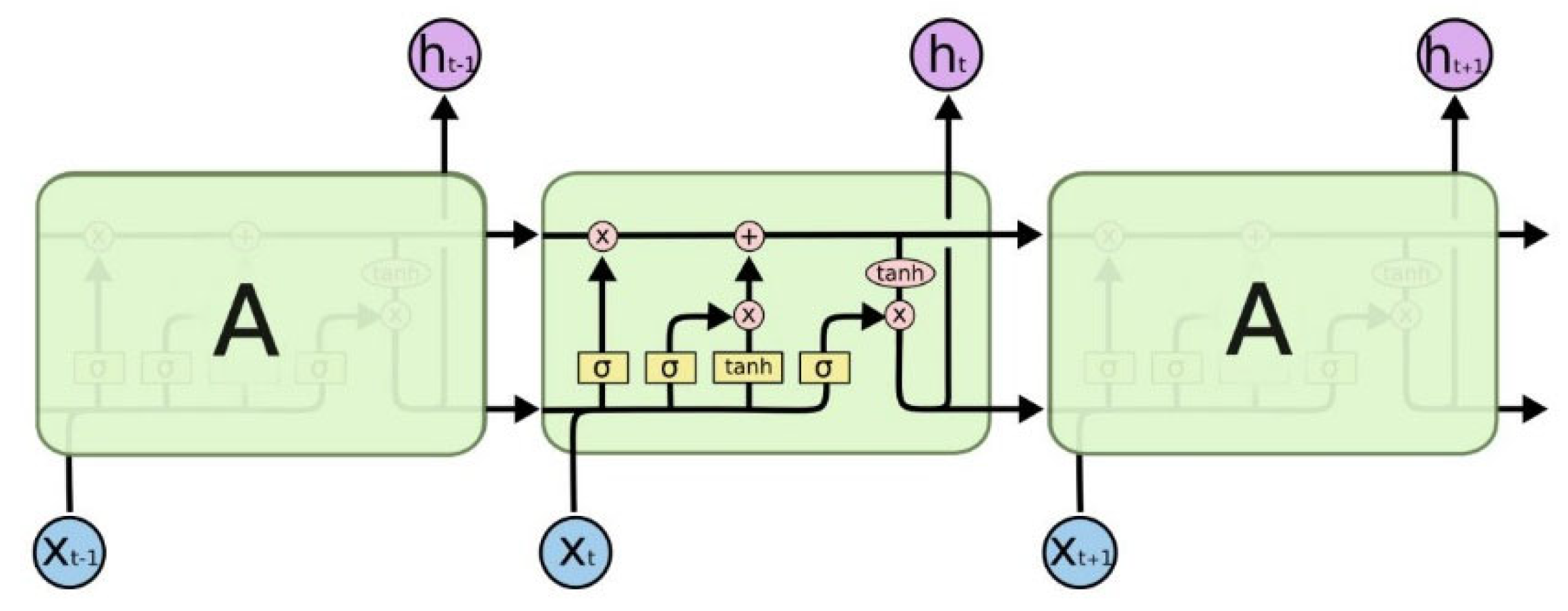
An LSTM model is a specific form of recurrent neural network (RNN), whereas (RNN) is designed to process sequence data [11,12]. Unlike the traditional neural network, the hidden layer of RNN is interconnected. This indicates that the current output is correlated to the previous output. Due to the correlation of option prices in different time, it is perfect for the research of option pricing. Experience shows that the RNN cannot ideally learn “long-term dependence”; therefore, an LSTM neural network was employed for option pricing. A typical LSTM scheme is shown in Figure 1.

Typically, an LSTM consists of the following gates [11,12].

Input gate: Information will first pass through the input gate after the data are imported. The switch will decide whether the information will be stored according to the state of the cell. Input gate comprises two steps. Firstly, the sigmoid layer will decide which data should be updated. Secondly, the tanh layer will produce new information C_t. It will possibly be added to the cell state.

Output gate: This gate decides how much information could be output. Firstly, an initial output is produced by the sigmoid layer, using tanh to scale C_t to [−1, 1]. Finally, the output of the model can be gained by multiplying the output obtained by sigmoid pair by pair.

Forget gate: This is controlled by sigmoid in the forget gate. It decides whether to let the obtained information (C_t−1) pass according to a ft value, which ranges between 0 and 1. The LSTM neural network has an LSTM layer. It affects not only the output layer but also the adjacent neurons in the same layer. Since the financial data are not independent, the current price will affect the future price, so the existence of the LSTM layer is necessary.

• Activation function

The activation function [11,12] is divided into “Saturated” and “Non-Saturated”. It uses the non-saturated function to solve the problem of the vanishing gradient of the neural network, and secondly, it can speed up the convergence.

The ideal activation function should satisfy two conditions: First, the mean of the output distribution should be zero, which would help to speed up the training process. Second, the activation function is one-sided saturated, which would improve the astringency of the model.

ReLU is one-sided saturated, but the mean of the distribution is not 0, while the mean of the Leaky ReLU is 0 but is two-sided saturated. Moreover, the ELU satisfies both conditions.

• ReLU (Rectified Linear Unit)

$$f\left(x\right)=\{ \begin{array}{c}x, if x>0\\ 0, if x\le 0\end{array}$$

(7)

• Leaky ReLU

$$f\left(x\right)=\{\begin{array}{c}x, if x>0\hfill \\ \alpha x, if x\le 0, \alpha =0.1\hfill \end{array}$$

(8)

• ELU (Exponential Linear Unit)

$$f\left(x\right)=\{ \begin{array}{c} x, if x>0\hfill \\ \alpha \left(e^x-1\right), if x\le 0\hfill \end{array}$$

(9)

In this research, we have constructed a network with four hidden layers of 120 nodes each. The loss function used is mean squared error (MSE), and the optimization uses the RMSprop algorithm. The activation function of the last layer is an exponential function.

2.3. Regulated LSTM Simulation

This part incorporates technical indicators [29,30] into the original LSTM. Due to the huge number of technical indexes, 25 indexes were selected and added to the original LSTM model to improve the accuracy of the model. There are two methods: F-Regression, and Mutual Information Regression. Both methods are used to jointly select the features. Finally, 25 optimal technical indicators were identified by taking the results shared by the two methods. Due to space constraint of the paper, we only describe seven technical indicators below.

2.3.1. Technical Indicators

Technical analysts forecast the option price in the future by using the technical indicators after analyzing the past information. These indicators could apply for all of the financial products possessing historical trading, including stocks, commodities, currencies and other securities. The technical indicators do not focus on the basis of the business, such as revenue and profit margins.

There are two basic types of technical indicators: Overlay—technical indicators that plot at the top of the price in the chart and use the same size of the price, and oscillation—technical indicators that plot above or below the price chart and oscillate between local minimum and maximum values. The technical indicators are added to regulate the original LSTM model to achieve better accuracy.

• Williams Percent Range (Williams% R)

Williams% R is a momentum indicator, which is called William Percent Range. It reflects the levels of overbought and oversold, and the range is between 0 and −100. If the result is above −20, it means overbought. If the reading is below −80, it represents oversold.

• Money Flow Index (MFI)

The Money Flow Index (MFI) is a technical oscillator, with the range from 0 to 100. It is used to find overbought and oversold for a financial product. A reading below 20 is regarded as oversold, and a reading above 80 is regarded as overbought.

• Price Rate of Change (ROC)

ROC is also called the Price Rate of Change, which is a momentum indicator. It is an unbounded oscillator that is used for technical analysis to set against a midpoint of the zero level.

• Chaikin Money Flow (CMF)

CMF is a technical indicator, which is called Chaikin Money Flow. It measures the money flow during a specific period of time. The range of Chaikin Money Flow is between 1 and −1. CMF can be used to quantify changes in buying and selling pressures and predict future changes and look for trading chances.

• Chande Momentum Oscillator (CMO)

CMO is a technical momentum indicator, with a range between −100 and +100. It is also called the Chande Momentum Oscillator.

• Detrended Price Oscillator (DPO)

DPO shows the peak and trough of the price, which is called the Detrended Price Oscillator. Traders usually use the DPO to simulate the buy and sell points according to the historical period.

The remaining technical indicators used in this research can be released upon request by readers.

2.3.2. Optimal Selections of Technical Indicators

In this section, we illustrate the general procedure for optimally identifying the technical indicators mentioned in the above section. We believe that not all the technical indicators influence option prices significantly, and the determination of key TIs is critical for improving the prediction accuracy of options by using LSTM. Therefore, we first integrate individual technical indicators with the LSTM to price the options and then conduct F-regression and MI regression separately in order to determine the scores for the contribution weights of the technical indicators on financial options. The process is lengthy and involves grouping of various TIs and various types of options.

Table 1. Options with F-regression.

TIs	Score
ROC_56	3684.859
RSI_56	3434.026
CMO_56	3422.589
KST_56	2607.816
DX_56	2267.488
CCI_56	2159.798
KDJK_56	2151.685
RSV_56	2034.888
WR_56	2034.888
MFI_56	1888.237
TRIX_56	1715.286
HMA_0	752.5516

and

Table 2. Options with MI regression.

TIs	Score
ROC_56	0.217495
WR_56	0.205305
RSV_56	0.204443
KST_56	0.203183
RSI_56	0.202899
CMO_56	0.199681
CCI_56	0.196113
TRIX_56	0.182988
HMA_0	0.181470
DX_56	0.180711
KDJK_56	0.172671
MFI_56	0.167238

illustrate some of the technical indicators, which yielded high (sorted) scores given by both the F-regression and the MI regression when pricing options. We pick such indicators as features for training the LSTM model.

2.4. Risk Measurements for Options

Due to the large amount of calculation required by the model, it is difficult to estimate the model’s degree of fit, but the accuracy of the pricing needs to be measured and compared. The following accuracy measurements are used, which mirror the degree of closeness between two variables.

• ME (Mean Error)

ME measures the difference between the observed value and the true value. It also commonly applies to the results predicted by machine learning.

$$ME=\left(\frac{1}{n}\right){\displaystyle \sum }_{i=1}^n{\left(C^{mark}-C^f\right)}^{}$$

(10)

where $C^{mark}$ is market price of option, $C^f$ is forecast price and n is the number of elements in the sample.

• RMSE(Root Mean Squared Error)

RMSE measures a mean value of the sum of square from which the data deviate from the actual value. RMSE can evaluate the degree of variation of data. The smaller the RMSE, the better the model quality and the more accurate the prediction is. Because there are frequent comparisons between different financial models, RMSE is widely used to measure the degree of accuracy.

$$RMSE=\sqrt{\left(\frac{1}{n}\right){\displaystyle \sum }_{i=1}^n{\left(C^{mark}-C^f\right)}^2}$$

(11)

where $C^{mark}$ is market price of option, $C^f$ is forecast price and n is the number of elements in the sample.

• MAE(Mean Absolute Error)

MAE is the average value of the absolute error, which can reflect the actual condition of the error of the predicted value.

$$MAE=\left(1/n\right){\displaystyle \sum }_{i=1}^n\left|C^{mark}-C^f\right|$$

(12)

• MAPE (Mean Absolute Percentage Error)

The value of MAPE is expressed as a percentage instead of a proportion. It can be used to compare predictions in different percentages.

$$MAPE=\frac{100\%}{n}{\displaystyle \sum }_{i=1}^n\left|\frac{C^{mark}-C^f}{C^{mark}}\right|$$

(13)

where $C^{mark}$ is market price of option, $C^f$ is forecast price and n is the number of elements in the sample.

As shown above, the predicted SSE 50 ETF option prices are critically checked against their market prices using these risk measures, and options with different maturity times and strike prices in this research are predicted in order to obtain the pricing errors statistically.

3. Empirical Analysis

The empirical data selected span more than 3 months for option maturity time from 1 January 2018 to 31 December 2019, which covers the data of the SSE 50 ETF for about two years. There are overall 44,604 columns of data, including the call options of 22,302 columns and the put options of 22,302 columns. An important factor called “risk-free interest rate” is selected from 1 January 2018 to 15 April 2021. The analysis chooses a period of two years.

As illustrated in

Table 3. Typical SSE50 ETF Call Options.

Code	Date	Open	High	Low	Close	K	Maturity
510050C1806M02650	2 January 2018	0.3332	0.3575	0.3332	0.3575	2.65	27 June 2018
510050C1806M02650	3 January 2018	0.3637	0.3788	0.3568	0.3573	2.65	27 June 2018

and

Table 4. Typical SSE50 ETF Put Options.

Code	Date	Open	High	Low	Close	K	Maturity
510050P1806M02650	2 January 2018	0.0355	0.0355	0.0187	0.0249	2.65	27 June 2018
510050P1806M02650	3 January 2018	0.024	0.0247	0.02	0.0215	2.65	27 June 2018

, typical call options and put option are tabled, respectively, concerning their prices, strike price K and maturity time. For option pricing using the described models, we select five variables as inputs, i.e., the price of underlying asset, the time to the expiration date, risk-free interest rate, historical volatility and strike price. The option price is the output variable of the model. Firstly, the option data are processed to calculate the dates and convert them into years. A risk-free interest rate is then converted to data with the percent unit removed. At the same time, we use the Min–Max Scaler to scale the date to the range between 0 and 1 (note: we need to rescale the data to the original domain for option prices). We re-group the whole data-set so that 70% of the data are used as the training set and 30% of the data are used as the test set. Next, the data of the training set are classified so that 70% of the training set is taken as the input set of the training model and 30% as the validation set of the validation model. After defining the activation function, we train the original model. When training the models, we also used two methods: Early Stopping and Model Checkpoint [31]. If loss is found to be increasing instead of decreasing during training, over-fitting may occur. The learning rate can be reduced by setting the “min delta”. We define “epochs = 100”, meaning that the LSTM networks run up to 100 times. In this research, the optimization of the hyperparameters [32] of the LSTM has not been implemented, and selections of these parameters depend on our experience obtained in the computations. As mentioned earlier, the number of epochs is 100, the batch size is 64 and the number of hidden neurons is 120. Such networks provide us with acceptable convergence time and accuracy. The training error is not important since we are looking for the models’ generalization capability. At the end of training, we calculate the risk measures of the training set, validation set and the test set.

Table 5. Comparisons of pricing risk measures between models for call options.

Call Options
B-S		LSTM			Regulated LSTM
	Predict	Train	Predict	Test	Train	Predict	Test
ME	0.012715	0.000651	0.000717	0.000681	0.000375	0.000377	0.000377
RMSE	0.112762	0.025505	0.026768	0.026092	0.019355	0.019405	0.019407
MAE	0.095152	0.019400	0.020273	0.019916	0.014932	0.014828	0.014917
MAPE	0.554104	0.127533	0.131535	0.129728	0.096781	0.095356	0.096492

and

Table 6. Comparisons of pricing accuracy between models for put options.

Put Options
B-S		LSTM			Regulated LSTM
	Predict	Train	Predict	Test	Train	Predict	Test
ME	0.004177	0.000713	0.000723	0.000714	0.000281	0.000309	0.000280
RMSE	0.064628	0.026709	0.026897	0.026717	0.016751	0.017582	0.016747
MAE	0.049610	0.019972	0.020071	0.020023	0.011727	0.012066	0.011716
MAPE	0.372994	0.158781	0.155234	0.157046	0.098828	0.102002	0.099301

give the pricing accuracies of the models.

It can be seen from the tables that for both the SSE50 ETF call and put options, the B-S model yields the highest errors, as expected. The ordinary LSTM without technical regulators performed better than the B-S model. For instance, for the call options, the pricing error RMSE given by the B-S model is 0.112762, while the pricing error produced by the ordinary LSTM is 0.026768, which is an improvement of 76.3% in terms of pricing accuracy. We can observe a similar improvement for the put options. On the other hand, the regulated LSTM outperforms the ordinary LSTM. Taking the same case, the regulated LSTM yields a pricing error of 0.019405, which corresponds to an improvement of 27.5% in terms of prediction accuracy. It can be observed in the tables that all the risk measures give us consistent results for the call and put options, which lead us to draw a conclusion that the regulated LSTM is superior over both the ordinary LSTM and the B-S model.

4. Conclusions

At present, the application of artificial neural networks in option pricing has attracted considerable attention. Artificial neural networks are widely used in various disciplines, while financial risks of options have become the main focus of this research. In terms of option risks in this paper, traditional and regulated LSTM neural networks are employed to predict option prices and compared with the conventional B-S model. The results show that the prediction ability of LSTM neural network is better than that of the B-S model. To overcome the weakness of the LSTM for option pricing with only options’ parameters as training features, we offer researchers and practitioners an alternative way to incorporate technical indicators in the LSTM. Further, we have also emphasized selections of optimal technical indicators using two statistical methods, i.e., F-Regression and Mutual Information. The paper demonstrates that these statistical methods can help determine the most influential TIs and discard some other TIs that have no strong effects on option prices. We can further conclude based on the research that (1) the artificial neural network-LSTM model is more accurate than the traditional option pricing model, i.e., the BS model, and that, (2) compared with the original LSTM model, the regulated/improved LSTM model incorporating technical indicators achieves better predictive ability. This research is therefore valuable for option risk management for both practitioners and researchers. Our future research will look into issues of optimization of LSTM hyperparameters and implementation of a stochastic option model as a new benchmark for financial options that with a long maturity time.

References

- Bachelier, L. Theorie de la speculation. Ann. Sci. De L’ecole Norm. Super. Ser. 1900, 3, 21. [Google Scholar] [CrossRef]
- Black, F.; Scholes, M.S. The pricing of options and corporate liabilities. J. Political Econ. 1973, 81, 637. [Google Scholar] [CrossRef] [Green Version]
- Benaroch, M.; Kauffman, R.J. Justifying electronic banking network expansion using real options analysis. MIS Q. 2000, 24, 197. [Google Scholar] [CrossRef] [Green Version]
- Kou, S. A jump diffusion model for option pricing. Manag. Sci. 2002, 48, 1086. [Google Scholar] [CrossRef] [Green Version]
- Carr, P.; Wu, L. Time-changed levy processes and option pricing. J. Financ. Econ. 2003, 71, 113. [Google Scholar] [CrossRef] [Green Version]
- Yao, J.; Li, Y.; Tan, C.L. Option price forecasting using neural networks. Omega-Int. J. Manag. Sci. 2000, 28, 455. [Google Scholar] [CrossRef]
- Lin, C.T.; Yeh, H.Y. The valuation of Taiwan stock index option price—Comparison of performances between Black-Scholes and neural network model. J. Stat. Manag. Syst. 2004, 8, 355. [Google Scholar] [CrossRef]
- Tan, D. S&P 500 index option pricing based on the BP neural networks. Stat. Inf. Forum 2008, 23, 40. [Google Scholar]
- Liu, D.; Huang, S. The performance of hybrid artificial neural network models for option pricing during financial crises. J. Data Sci. 2016, 14, 1. [Google Scholar] [CrossRef]
- Wang, L.L.; Li, Y. Research on option pricing of shanghai stock exchange 50ETF based on neural network. Comput. Knowl. Technol. 2020, 16, 196. [Google Scholar]
- Hochreiter, S.; Schmidhuber, J. Long short-term memory. Neural Comput. 1997, 9, 1735. [Google Scholar] [CrossRef] [PubMed]
- Graves, A.; Schmidhuber, J. Framewise phoneme classification with bidirectional LSTM and other neural network architectures. Neural Netw. 2005, 18, 602. [Google Scholar] [CrossRef] [PubMed]
- Xie, H.L.; You, T. Research on European Stock Index options pricing based on deep learning algorithm: Evidence from 50ETF options markets. Stat. Inf. Forum 2018, 33, 99. [Google Scholar]
- Fischer, T.; Krauss, C. Deep learning with long short-term memory networks for financial market predictions. Eur. J. Oper. Res. 2018, 270, 654–669. [Google Scholar] [CrossRef] [Green Version]
- Zhu, B.; Pan, L. Test and analysis of a stock price forecasting indicator. Econ. Manag. 2003, 2, 68–73. [Google Scholar]
- Ko, K.C.; Lin, S.J.; Su, H.J.; Chang, H.H. Value investing and technical analysis in Taiwan stock market. Pac. -Basin Financ. J. 2014, 26, 14–36. [Google Scholar] [CrossRef]
- Nelson, D.M.Q.; Pereira, A.C.M.; de Oliveira, R.A. Stock market’s price movement prediction with LSTM neural networks. In Proceedings of the 2017 International Joint Conference on Neural Networks (IJCNN), Anchorage, AK, USA, 14–19 May 2017; pp. 1419–1426. [Google Scholar]
- Mohanty, D.K.; Parida, A.K.; Khuntia, S.S. Financial market prediction under deep learning framework using auto encoder and kernel extreme learning machine. Appl. Soft Comput. 2020, 99, 106898. [Google Scholar] [CrossRef]
- Yıldırım, D.C.; Toroslu, I.H.; Fiore, U. Forecasting directional movement of Forex data using LSTM with technical and macroeconomic indicators. Financ. Innov. 2021, 7, 1. [Google Scholar] [CrossRef]
- Piravechsakul, P.; Kasetkasem, T.; Marukatat, S.; Kumazawa, I. Combining Technical Indicators and Deep Learning by using LSTM Stock Price Predictor. In Proceedings of the 18th International Conference on Electrical Engineering/Electronics, Computer, Telecommunications and Information Technology (ECTI-CON), Chiang Mai, Thailand, 9–22 May 2021. [Google Scholar]
- Chriss, N.A.; Kawaller, I. Black-Scholes and Beyond: Option Pricing Models, 1st ed.; McGraw-Hill: New York, NY, USA, 1996. [Google Scholar]
- Barndorff-Nielsen, O.E.; Stelzer, R. The Multivariate supOU Stochastic Volatility Model. Ole Eiler Barndorff-Nielsen, Robert Stelzer. Math. Financ. 2013, 23, 275–296. [Google Scholar] [CrossRef] [Green Version]
- Chorro, C.; Guégan, D.; Ielpo, F. Option pricing for GARCH-type models with generalized hyperbolic innovations. Quant. Financ. 2012, 12, 1079–1094. [Google Scholar] [CrossRef] [Green Version]
- Ramponi, A. Spread Option Pricing in Regime-Switching Jump Diffusion Models. Mathematics 2022, 10, 1574. [Google Scholar] [CrossRef]
- Ma, C.; Yue, S.; Ren, Y. Pricing Vulnerable European Options under Lévy Process with Stochastic Volatility. Discret. Dyn. Nat. Soc. 2018, 3402703. [Google Scholar] [CrossRef] [Green Version]
- Schoutens, W. Lévy Processes in Finance: Pricing Financial Derivatives, 1st ed.; Wiley: Hoboken, NJ, USA, 2003. [Google Scholar]
- Liu, D. Markov modulated jump-diffusions for currency options when regime switching risk is priced. Int. J. Financ. Eng. 2019, 6, 1950038. [Google Scholar] [CrossRef]
- China Assets Management Co Ltd. China 50 ETF. Available online: https://fund.chinaamc.com/portal/cn/uploadFiles/50ETF.1253167410245.pdf (accessed on 20 April 2022).
- A List of Technical Indicators. Available online: https://www.tradingtechnologies.com/xtrader-help/x-study/technical-indicator-definitions/list-of-technical-indicators/ (accessed on 12 April 2021).
- Salkar, T.; Shinde, A.; Tamhankar, N.; Bhagat, N. Algorithmic Trading using Technical Indicators. In Proceedings of the 2021 International Conference on Communication Information and Computing Technology (ICCICT), Mumbai, India, 25–27 June 2021; Available online: https://ieeexplore-ieee-org.ez.xjtlu.edu.cn/stamp/stamp.jsp?tp=&arnumber=9510135 (accessed on 28 November 2021).
- Brownlee, J. Better Deep Learning: Train Faster, Reduce Overfitting, and Make Better Predictions; Machine Learning Mastery. 2018. Available online: https://machinelearningmastery.com/better-deep-learning/#packages (accessed on 21 April 2022).
- Chen, Z.; Yang, C.; Qiao, J. The optimal design and application of LSTM neural network based on the hybrid coding PSO algorithm. J. Supercomput. 2022, 78, 7227–7259. [Google Scholar] [CrossRef]
Figure 1.
The repeating module in an LSTM contains four interacting layers.