Modeling and Forecasting Cryptocurrency Closing Prices with Rao Algorithm-Based Artificial Neural Networks: A Machine Learning Approach

Abstract

Artificial neural networks (ANNs) are suitable procedures for predicting financial time series (FTS). Cryptocurrencies are good investment assets; therefore, the effective prediction of cryptocurrencies has become a trending area of research. Capturing inherent uncertainties associated with cryptocurrency FTS with conventional methods is difficult. Though ANNs are the better alternative, fixing the optimal parameters of ANNs is a tedious job. This article develops a hybrid ANN through Rao algorithm (RA + ANN) for the effective prediction of six popular cryptocurrencies such as Bitcoin, Litecoin, Ethereum, CMC 200, Tether, and Ripple. Six comparative models such as GA + ANN, PSO + ANN, MLP, SVM, LSE, and ARIMA are developed and trained in a similar way. All these models are evaluated through the mean absolute percentage of error (MAPE) and average relative variance (ARV) metrics. It is found that the proposed RA + ANN generated the lowest MAPE and ARV values, statistically different as compared with existing methods mentioned above, and hence can be recommended as a potential financial instrument for predicting cryptocurrencies.

1. Introduction

Cryptocurrency is a virtual or digital currency that is meant to be a means of exchange for online transactions to purchase goods and services. An online ledger is used with strong cryptography for securing online transactions. Cryptos evince a lot of interest today because they are traded for-profit and because of the rich and growing valuations in relatively shorter periods of time. While these currencies are unregulated, many of the international governments and countries, after an early period of denial, are now showing signs of the adoption of some of the other forms of cryptocurrencies for transactions. Without any bank or any central authority, these cryptos are built on a decentralized or distributed peer-to-peer network. Cryptocurrencies have certain special characteristics [1]. They use decentralized control, so central authority is not required.

To avoid dispute, it ensures pseudo-anonymity. Since the reproduction of digital currency is easy, double-spending attack protection is ensured.

While Bitcoin was the earliest and most popular one [2], there are also many others, which are continuing to grow in user base, popularity, and market share, such as Ethereum, Tether, CMC 200, Ripple, Polkadot, XRP, Cardano, Chainlink, Litecoin, Bitcoin Cash, Binance Coin, etc. As the cryptocurrency market prices are growing fast and behave similarly to stock market price movement, investors, as well as researchers, are concerned about the proper prediction of cryptocurrencies market values. The principle of cryptography is the basis of the decentralized digital currency having an open source. The relevance of cryptocurrencies as an emerging market in the financial world is escalating significantly. Nowadays, more and more financial organizations are getting concerned about cryptocurrency trading. The trading opportunities and profitability in the cryptocurrency market are studied in [3]. A survey on systems of cryptocurrency is elaborated in [4]. The characteristics of this market, such as the high availability of market data, high volatility, smaller capitalization, and decentralized control, are studied in the literature [5]. Despite the fact that this market acts similarly to other stock markets in terms of intrinsic volatility, investor confidence has been reflected in it [6,7,8]. The feasibility of this market in relation to other financial markets is documented in the literature [9,10]. Similarly, to another stock market, cryptocurrency market prices behaved arbitrarily and with high nonlinearity and dynamics. Though few computational intelligence models are available for the prediction of cryptocurrencies, sophisticated methods with accurate prediction abilities are still missing and need to be searched. From the literature, it is observed that different stock market predictions have been made successively by different ANN techniques [11,12,13,14,15,16]. Motivated by such works in the last few years, different soft computing methods are suggested in the literature to predict cryptocurrencies indices. Soft computing techniques, such as Long short-term memory neural networks and MLP [17], Random walk theory [18], Support vector machines [19], etc., are already used to forecast cryptocurrencies. The recurrent neural network was also used for entrapping threats in cryptocurrency [20]. Few machine learning and statistical methodologies are found in the literature for the prediction of Bitcoin [21,22,23,24,25]. Several data-driven and machine learning approaches are developed in the literature for industrial and agricultural applications. A data-driven prognosis approach for the prediction of run-to-failure low-speed slew bearing vibration data is proposed in [26]. A machine learning-based method is proposed in [27] for clay prediction technology. A hybrid architecture is proposed in [28] for the minimization of energy consumption and elapsed time for IoT workloads. The forecasting accuracy of a neural model is greatly subjective to the network magnitude and learning method. Gradient descent learning is a common method for neural network training. The typical downsides of this technique are that it has a slow convergence rate, imperfect learning, and is prone to local minima. It adds computational overhead to the model. Therefore, evolutionary optimization techniques are used to train the ANN and claim superior to [29,30]. The improper selection of algorithm-specific parameters of evolutionary optimization methods may land them at local optima or inaccurate solutions. To eradicate this, a good number of swarm and evolutionary optimization techniques are groomed up and heavily used for ANN training. These techniques are broadly termed nature-inspired optimization algorithms because they mimic natural processes. Certain algorithms, such as genetic algorithms, differential evolution, and evolution strategy, are based on the theory of natural evolution. Few algorithms simulate the behavior of swarms, insects, etc., such as particle swarm optimization, ant colony optimization, artificial bee colony optimization, bacterial foraging optimization, monarch butterfly optimization, and so on. Some other techniques are bio-geography optimization, gravitational search algorithm, multi-verse optimization [31], fireworks algorithm [32,33], chemical reaction optimization [34,35], etc. Though such nature-inspired optimization techniques have been used for solving several complex problems, their efficiency is determined by well-adjustable learning parameters. In the quest to search for the optimal global solution, the selection of appropriate learning parameters makes the technique difficult to use. Choosing optimal learning parameters for any particular problem requires a number of trial-and-error methods. The improper selection of algorithm-specific parameters may land the search operation at local optima or inaccurate solutions. As a result, an optimization technique with higher approximation capability but fewer learning parameters will be of relevance for better forecasting accuracy. Recently, few methods have been developed for constrained and unconstrained optimization problems, which are claimed to be simple as well as parameter-free algorithms, such as teaching learning-based optimization [36] and Jaya algorithm [37]. With the objective of developing simple and effective optimization techniques, Rao proposed metaphor-less algorithms called Rao algorithms [25], where algorithm-specific learning parameters are not required, i.e., these algorithms are free from learning parameters. Only the initialization of population size is enough. The algorithms keep on finding the best and the worst solution from the selected population and initiate random interaction among the candidate solutions. Very soon, these algorithms are applied to mechanical system components to obtain the design optimization [14,38,39], estimation of photovoltaic cell [40,41], optimal coordination of overcurrent relays [42], etc. However, Rao algorithms are not explored for the optimization of ANN parameters. This article attempts to test out the appropriateness of Rao algorithms on finding the optimal parameters of ANNs and applying the resultant method for stock closing price prediction.

The objectives of this article are highlighted as follows:

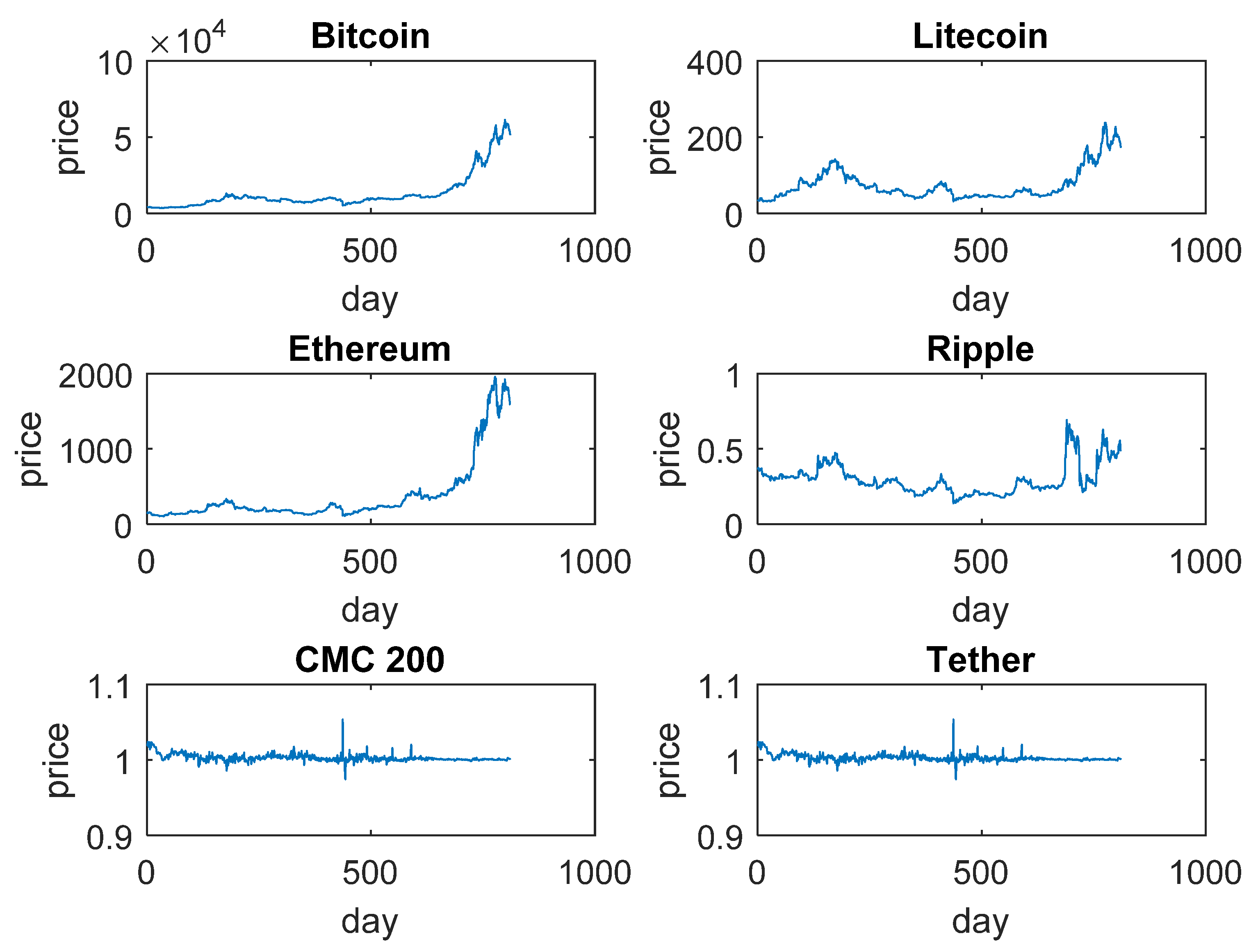
• We are designing an efficient ANN forecast for the nearly precise prediction of cryptocurrencies such as Bitcoin, Litecoin, Ethereum, CMC 200, Tether, and Ripple.
• Suitable tuning of ANN parameters (i.e., weight and bias) by RA, thus forming a hybrid model (i.e., RA + ANN) to overcome the limitations of derivative-based optimization techniques.
• We are evaluating the performance of the RA + ANN forecast through two performance metrics, MAPE and ARV.

The flow of the article is as follows. A concise description of ANNs is presented in Section 2. The proposed RA + ANN is described in Section 3. The experimental data are presented in Section 4. Section 5 contains the summarized results from the experimentation and analysis of outcomes, followed by concluding remarks.

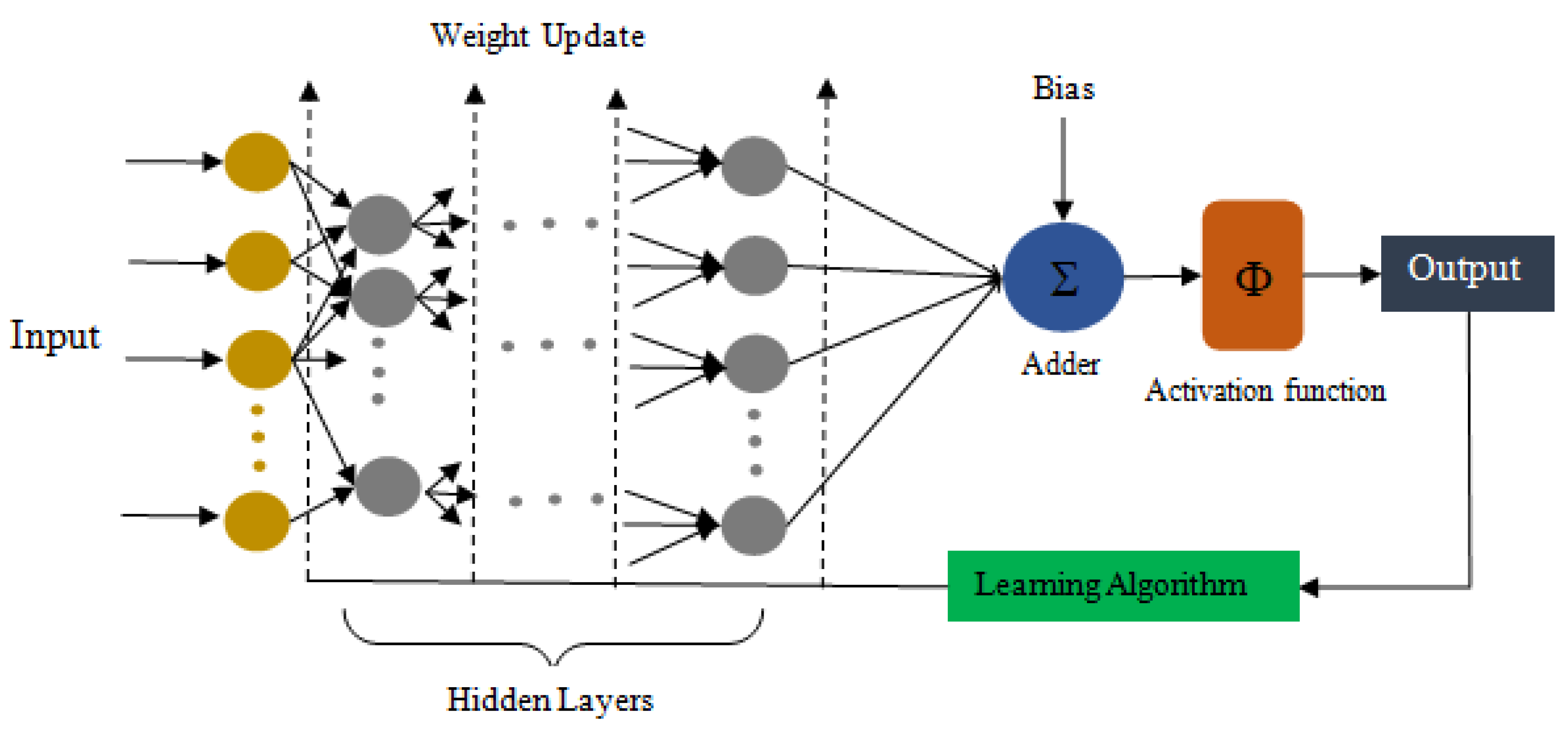
2. Artificial Neural Network

An ANN simulates the way the human brain works, making it different from conventional digital computers [43]. ANNs are also capable of complex data processing having neurons as computational units. ANNs have the capabilities of getting good approximation solutions to intractable problems, and they can also solve a very complex problem by decomposing it into smaller tasks, which makes them different from conventional computing.

The neural networks gain training by detecting the patterns in the data. As the human brain consists of billions of neurons, fully interconnected by synapses, similarly ANNs consist of hundreds of processing units as artificial neurons, which are fully connected through neural links. The Schematic block diagram (Figure 1) represents the basic ANN architecture with some hidden layers of neurons and one output layer neuron.

Supervised learning is used for error correction in this case, i.e., the expected response for the given inputs is submitted at the output neuron to calculate the error. In the time-series data to speculate one-day-ahead index, a single output unit model is used. A linear transfer function is used in the input layer. The hidden and output layer neurons contain nonlinear activation functions. Here, we have taken nonlinear activation as sigmoidal function in (1), i.e.,:

$${\mathrm{y}}_{\mathrm{out}}=\frac{1}{1+{\mathrm{e}}^{-{\mathsf{\lambda }\mathrm{y}}_{\mathrm{in}}}}$$

(1)

where ${\mathrm{y}}_{\mathrm{out}}$ and ${\mathrm{y}}_{\mathrm{in}}$ represent the output and input of the neuron $\mathrm{y}$, respectively, and λ acts as the sigmoidal gain. In the input layer, let there be $\mathrm{n}$ neurons. The input layer stands for the input variable of the problem. Each input variable input layer contains one-one node. The hidden layers are helpful in capturing the nonlinearity among variables. In the hidden layer output ${\mathrm{y}}_{\mathrm{j}}$ is computed using (2) for each neuron j,

$${\mathrm{y}}_{\mathrm{j}}=\mathrm{f}\left({\mathrm{b}}_{\mathrm{j}}+{\displaystyle \sum }_{\mathrm{i}=1}^{\mathrm{n}}{\mathrm{w}}_{\mathrm{ij}}{\ast \mathrm{x}}_{\mathrm{i}}\right)$$

(2)

where $\mathrm{f}$ stands for a nonlinear activation function, ${\mathrm{b}}_{\mathrm{j}}$ is the bias value, ${\mathrm{x}}_{\mathrm{i}}$ represents the ${\mathrm{i}}^{\mathrm{th}}$ component of the input vector,${\mathrm{w}}_{\mathrm{ij}}$ is the synaptic weight connecting ${\mathrm{i}}^{\mathrm{th}}$ input neuron and ${\mathrm{j}}^{\mathrm{th}}$ hidden neuron.

Suppose there are $\mathrm{m}$ numbers of neurons present in this hidden layer, then for the next hidden layer these $\mathrm{m}$ outputs become the input. Then (3) for each neuron $\mathrm{j}$ of the next hidden layer can be represented as,

$${\mathrm{y}}_{\mathrm{j}}=\mathrm{f}\left({\mathrm{b}}_{\mathrm{j}}+{\displaystyle \sum }_{\mathrm{i}=1}^{\mathrm{m}}{\mathrm{w}}_{\mathrm{ij}}{\ast \mathrm{y}}_{\mathrm{i}}\right)$$

(3)

This signal flows in the forward direction through each hidden layer until it reaches the node of the output layer.

For a single output neuron (4) is used to calculate the output ${\mathrm{y}}_{\mathrm{esst}}$

$${\mathrm{y}}_{\mathrm{esst}}=\mathrm{f}\left({\mathrm{b}}_{\mathrm{o}}+{\displaystyle \sum }_{\mathrm{j}=1}^{\mathrm{m}}{\mathrm{v}}_{\mathrm{j}}{\ast \mathrm{y}}_{\mathrm{j}}\right)$$

(4)

where ${\mathrm{b}}_{\mathrm{o}}$ is the bias for output node, the weighted sum calculated as in (2) is ${\mathrm{y}}_{\mathrm{j}}$, ${\mathrm{v}}_{\mathrm{j}}$ represents the synaptic weight between ${\mathrm{j}}^{\mathrm{th}}$ hidden neuron and output neuron.

Given a set of training samples $\mathrm{S}={\{{\mathrm{x}}_{\mathrm{i}},{\mathrm{y}}_{\mathrm{i}}\}}_{\mathrm{i}=1}^{\mathrm{N}}$ to train the ANN, let ${\mathrm{y}}_{\mathrm{i}}$ be the output of ${\mathrm{i}}^{\mathrm{th}}$ input sample, and ${\mathrm{y}}_{\mathrm{esst}}$ is the computed output of the same ${\mathrm{i}}^{\mathrm{th}}$ input, then using (5) the error is calculated as,

$${\mathrm{Error}}_{\mathrm{i}}={\mathrm{y}}_{\mathrm{i}}-{\mathrm{y}}_{\mathrm{esst}}$$

(5)

The error value that is produced by ${\mathrm{n}}^{\mathrm{th}}$ training sample at the output of neuron $\mathrm{i}$ is defined by (6) as,

$${\mathrm{Error}}_{\mathrm{i}}\left(\mathrm{n}\right)={\mathrm{y}}_{\mathrm{i}}\left(\mathrm{n}\right)-{\mathrm{y}}_{\mathrm{esst}}\left(\mathrm{n}\right)$$

(6)

Then the instantaneous error at neuron $\mathrm{i}$ is defined by (7) as,

$${\mathsf{\epsilon }}_{\mathrm{i}}\left(\mathrm{n}\right)=\frac{1}{2}{\mathrm{Error}}_{\mathrm{i}}{}^2\left(\mathrm{n}\right)$$

(7)

Hence the total instantaneous error of the whole network, $\mathsf{\epsilon }\left(\mathrm{n}\right)$ can be defined by the following (8) as,

$$\mathsf{\epsilon }\left(\mathrm{n}\right)={\displaystyle \sum }_{\mathrm{i}ϵ\mathrm{C}}{\mathsf{\epsilon }}_{\mathrm{i}}\left(\mathrm{n}\right)$$

(8)

Here $\mathrm{C}$ represents the set containing all the output layer neurons. In this paper, we have considered one neuron in the output layer. Therefore, here we can represent the network error in the neural network model as in (9),

$$\mathsf{\epsilon }\left(\mathrm{n}\right)={\mathsf{\epsilon }}_{\mathrm{i}}\left(\mathrm{n}\right)$$

(9)

The average error over the whole training sample in the neural network model can be defined by (10) as,

$${\mathsf{\epsilon }}_{\mathrm{av}}\left(\mathrm{N}\right)={\displaystyle \sum }_{\mathrm{n}=1}^{\mathrm{N}}\mathsf{\epsilon }\left(\mathrm{n}\right)$$

(10)

The optimal weight vector is computed by the weight update algorithm using error signal ${\mathrm{Error}}_{\mathrm{i}}$. In the training phase, the training set input vectors are repeatedly presented to the neural network model to update the weights and the biases by training algorithm. If the error is small enough per epoch, then no further training is required. Unfortunately, this criterion may lead to local minimum. Therefore, the performance of the network is tested for generalization performance after each iteration of training. Once the generalization performance is sufficient or adequate, the learning process is stopped. Therefore, the intent is to reduce the total error of Equation (5) with an optimized set of weight and bias vector of the ANN.

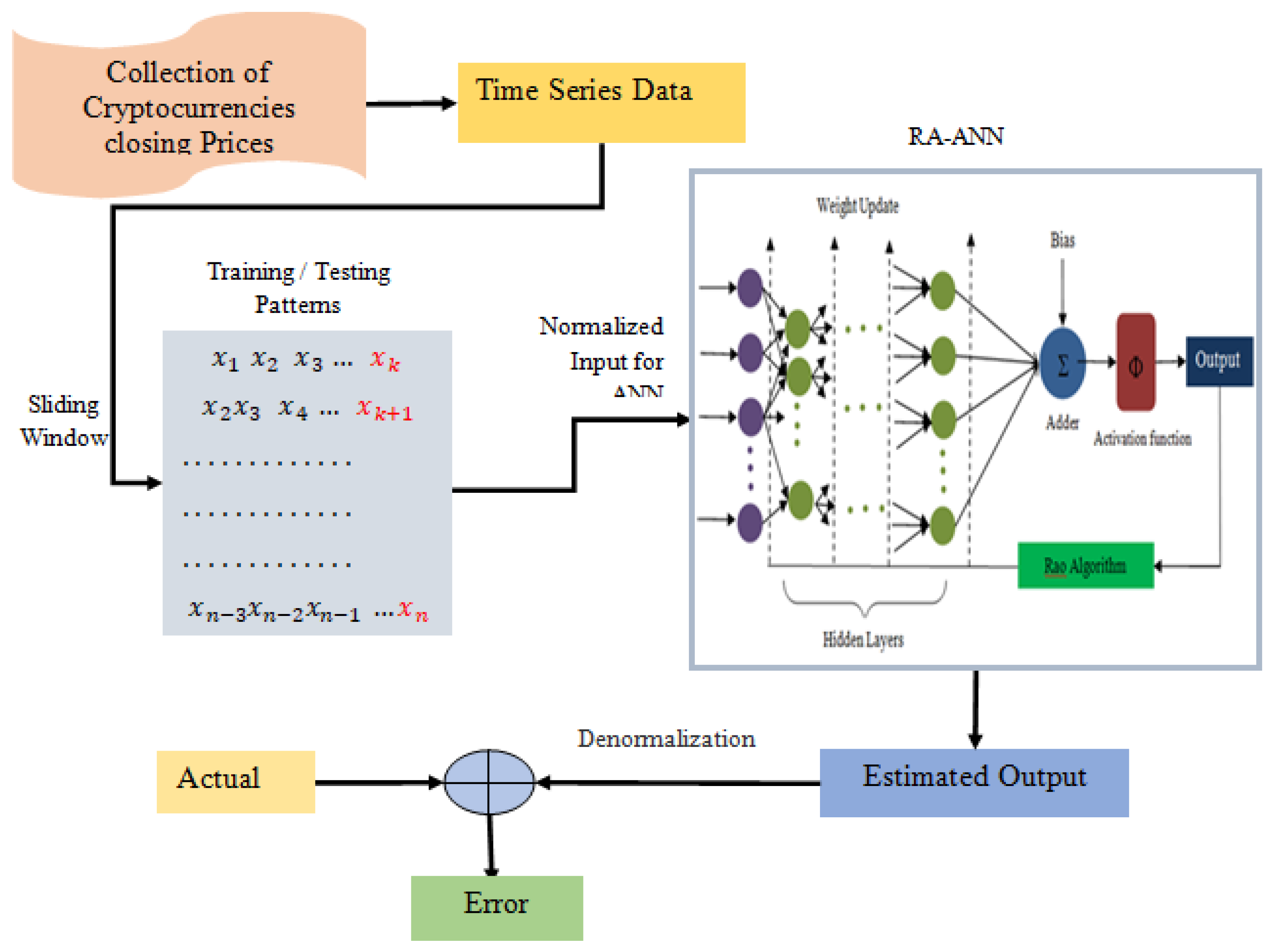
3. Proposed RA + ANN Based Forecasting

Rao algorithms are newly developed population-based optimization algorithms. Unlike other nature-inspired optimization techniques, these are not mimicking the behavior of swarms, animals, birds, or any physical or chemical phenomenon. Therefore, they are claimed as metaphor-less optimization techniques by the inventor [25]. Any algorithm-specific parameters are not required by these algorithms. Only specifying the number of candidate solutions, design variables, and termination criteria is sufficient to automate the search process. The techniques are simple, do not necessitate human intervention, and provide effective solutions to complicated problems. The algorithms are presented as follows.

Let $f\left(w\right)$ be an objective function that needs to be optimized (i.e., the error function to be minimized here). Let the population (search space of ANN model) have $n$ number of candidate solutions (weight and bias vector), each of which has $m$ number of design variables (weight values). Each candidate solution has a fitness value (i.e., error value), and the lower the error signal, the better is the solution. At any iteration $i$, let the best and worst solution of the population be $f{\left(w\right)}_{best }$ and $f{\left(w\right)}_{worst}$ respectively. The current value of a candidate solution (weight vector) at $i^{th }$ iteration is updated as per the following Equations (11)–(13) as,

$$W_{j,k,i}^{\prime }=W_{j,k,i}+ran{d}_{1,j,i}\ast \left(W_{j,best,i}-W_{j,worst,i}\right)$$

(11)

$$W_{j,k,i}^{\prime }=W_{j,k,i}+ran{d}_{1,j,i}\ast \left(W_{j,best,i}-W_{j,worst,i}\right)+ran{d}_{2,j,i}\ast \left(\left|W_{j,k,i} or W_{j,l,i}\right|-\left|W_{j,l,i} or W_{j,k,i}\right|\right)$$

(12)

$$W_{j,k,i}^{\prime }=W_{j,k,i}+ran{d}_{1,j,i}\ast \left(W_{j,best,i}-\left|W_{j,worst,i}\right|\right)+ran{d}_{2,j,i}\ast \left(\left|W_{j,k,i} or W_{j,l,i}\right|-W_{j,l,i} or W_{j,k,i}\right)$$

(13)

where:

• $W_{j,k,i }$ = the value of $j^{th}$ variable of $k^{th}$ solution ($k=1,2,3,\cdots ,n$) at $i^{th}$ iteration.
• $W_{j,k,i }^{\prime }$ = the modified value of $j^{th}$ variable of $k^{th}$ solution ($k=1,2,3,\cdots ,n$) at $i^{th}$ iteration.
• $W_{j,best,i}$ = $j^{th}$ variable value of the best solution in $i^{th }$ iteration.
• $W_{j,worst,i}$ = $j^{th}$ variable value of the worst solution $i^{th }$ iteration.
• $ran{d}_{1,j,i }$ and $ran{d}_{2,j,i}$ are two random values in [0,1].

The terms “$W_{j,k,i} or W_{j,l,i}$” in (11)–(13) represent the fitness comparison of $k^{th}$ candidate solution with that of $l^{th}$ solution, which is randomly drawn from the population. An information exchange occurs based on their fitness values. This ensures the communication among the candidate solutions. Based on the concept discussed, the RA + ANN-based forecasting can be explained by Algorithm 1. The pictorial description is given below (Figure 2).

Algorithm 1: RA + ANN-based forecasting.

1. Set population size (n), No. of design variables (m), and Termination criteria. 2. Initialization of population. 3. Set training and test data using sliding window. 4. Normalization of training and test data.   /* Model Training */ 5. While (! = termination criteria)        For each candidate solution (W) in the population.           Supply train data and W to ANN.           Compute ANN output.           Error = expected output–estimated output           Fitness = accumulated error.        End           Identify best and worst solution.           Update population using any Equations (8)–(10). 6. End   /* Model Testing */ 7. Feed test data and best solution to ANN.           Calculate the model output error value. 8. Reiterate Steps 2–6 for all training and test patterns and preserve total error.

The RA + ANN forecasting model works as follows: the cryptocurrency’s historical closing prices are collected. Approximately 60% of the total input data are pre-owned for training the neural net, and after the network is trained, the remaining 40% of the data is used for testing the correctness of the proposed model. The closing price data are collected and stored as time-series data. We have used the sliding window approach to generate the training and testing data sets. The input for the network is normalized in the range [0,1]. The normalized input is fed into the network to obtain an output. The difference between the computed output (estimated) and expected output (actual) gives an error. The Rao algorithm is used to update the weights to obtain the minimum error. The performance of the network is tested for generalization performance after each iteration of training. Here, Rao algorithms work on identifying the best and worst solution and interaction between contestants in the search space, i.e., the population. The lack of algorithm-specific parameters eliminates any human interventions. In Algorithm 1, the size of the population, design variables, and stopping criteria are needed to be fixed at the beginning. The size of the sliding window used to form training and test patterns is a matter of experimentation.

4. Cryptocurrency Data

The models are evaluated on experimenting with the cryptocurrency’s historical closing prices collected from https://www.CryptoDataDownload.com (accessed on 26 March 2021). The currencies are Bitcoin, Litecoin, Ethereum, CMC 200, Tither, and Ripple. The data are collected during the period from 1 January 2019 to 25 March 2021. A condensed statistic of the six datasets is gathered in

Table 1. Statistical summary of four cryptocurrencies.

Statistic	Bitcoin	Litecoin	Ethereum	Ripple	CMC 200	Tether
Minimum	68.4300	1.1600	0.4348	0.0028	0.9742	0.9742
Mean	1.4826 × 103	20.4966	147.7843	0.0984	1.0029	1.0029
Median	482.8100	3.9100	12.0200	0.0079	1.0017	1.0017
Variance	8.7535 × 106	2.2240 × 103	6.9765 × 104	0.1028	2.5621 × 10−5	2.5621 × 10−5
Maximum	1.9497 × 104	358.3400	1.3964 × 103	3.3800	1.0536	1.0536
Standard deviation	2.9593 × 103	47.1594	264.1308	0.3206	0.0051	0.0051
Skewness	3.5394	4.1627	2.3844	5.8039	1.9417	1.9417
Kurtosis	15.9671	21.5925	8.5122	42.9469	19.3797	19.3797
Correlation coefficient	0.00130	0.00211	−0.0052	0.0027	0.0039	0.0035

. The price series are plotted in Figure 3. The raw data are normalized using the sigmoid data normalization method [44].

5. Experimental Results and Analysis

To evaluate the models, we used them to forecast the prices of four cryptocurrency datasets separately. To access the capacity of the RA + ANN method, five other methods such as ANN trained by genetic algorithm (GA + ANN), particle swarm optimization trained ANN (PSO + ANN), MLP, SVM, ARIMA, and least squared estimator (LSE) are developed in this study and a comparison is performed.

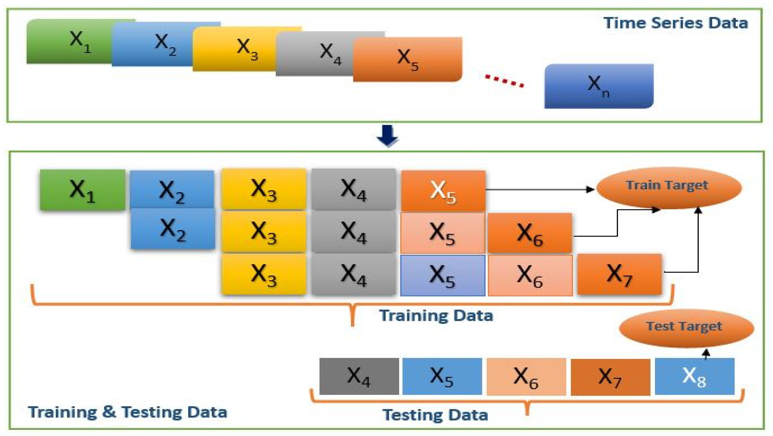
5.1. Model Input Selection and Normalization

A time series approach is used in this study. A rolling window method is used to generate the train and test patterns from the dataset. The method is depicted in Figure 4.

Each sample in the dataset is considered as a data point on the time series. A window of fixed size is rolled over the time series. On each movement, an old datapoint is dropped and a new datapoint is included, as shown in Figure 4. The number of datapoints included by the window at any instant of time is considered as one training sample for the model. The width of the window is determined experimentally. For example, one train/test set is formed by the rolling window of width three, as follows.

$$\underset{\underset{Trainingdata}{⏟}}{\begin{array}{cc}\begin{array}{ccc}x\left(k\right)& x\left(k+1\right)& x\left(k+2\right)\\ x\left(k+1\right)& x\left(k+2\right)& x\left(k+3\right)\\ x\left(k+2\right)& x\left(k+3\right)& x\left(k+4\right)\end{array}& \begin{array}{c}⋮\\ ⋮\\ ⋮\end{array}\end{array}}\underset{Target}{\underbrace{\begin{array}{c}x\left(k+3\right)\\ x\left(k+4\right)\\ x\left(k+5\right)\end{array}}}$$

$$\underset{Testdata}{\underbrace{\begin{array}{cccc}x\left(k+3\right)& x\left(k+4\right)& x\left(k+5\right)& \begin{array}{c}⋮\end{array}\end{array}}}\underset{Target}{\underbrace{x\left(k+6\right)}}$$

Each input pattern is then normalized to scale the data into same range for each input feature to diminish the bias [44,45]. The $tanh$ normalization method as in Equation (14) is used to standardize the input data. The mean and standard deviation of a training pattern are represented as µ and σ respectively.

$$\widehat{x}=0.5\ast \left(tanh\left(\frac{0.01\ast \left(x-\mu \right)}{\sigma }\right)+1\right)$$

(14)

5.2. Performance Evaluation Metrics

The accuracy of all models is accessed through two mesures, i.e., Mean Absolute Percentage of Errors (MAPE) and Average Relative Variance (ARV), as in (15) and (16).

$$\mathrm{MAPE}=\frac{1}{N}{\displaystyle \sum }_{i=1}^N\frac{\left|x_i-{\widehat{x}}_i\right|}{x_i}\times 100\%$$

(15)

$$\mathrm{ARV}=\frac{{{\displaystyle \sum }}_{i=1}^N{\left({\widehat{x}}_i-x_i\right)}^2}{{{\displaystyle \sum }}_{i=1}^N{\left({\widehat{x}}_i-\overline{X}\right)}^{2 }}$$

(16)

5.3. Experimental Setting

The train and test patterns are generated as described in Section 5.1, and the same patterns are fed to all seven models separately. To overcome the biases of the models, each model is simulated twenty times, and the mean error value is recorded for comparisons. An ANN with one hidden layer is used as the base network. The input layer size is equal to the rolling window size, and the output layer has only one neuron, as there is one target output. However, the numbers of neurons in the hidden layer are decided experimentally. An inadequate number of hidden neurons may produce poor accuracy, whereas the excess number of such neurons adds computational overhead. Therefore, the size of the hidden layer impacts the model performance a lot and must be decided carefully. During experimentation, different possible values for the model parameters were tested, and the best values were recorded. The suitable parameter values obtained during the simulation process are called simulated parameters. For the MLP model, the learning rate (α) and momentum factor (µ) are set to 0.2 and 0.5, respectively. The number of iterations was fixed to 400, and gradient descent-based backpropagation learning was adopted for training. For SVM, we used the radial basis function as the kernel. For PSO + ANN, the total number of the particle was set to 100, the number of iterations was 250, learning factors were fixed to 3 each. Similarly, in the case of GA + ANN, the three critical parameters, i.e., population size, crossover, and mutation probabilities, are considered as 80, 0.7, and 0.02, respectively. The stopping condition is the maximum number of generations, i.e., 200. Binary encoding is used for individual encoding, and elitism is used as the selection method. However, the RA + ANN used only 50 candidate solutions and 100 number iterations to reach the global optima. All the experimentations are performed with a system of Intel core i3 CPU, 2.27GHz and 8.0 GB memory, and a Matlab-2015 program writing environment.

5.4. Simulation Results and Discussion

The mean values from twenty simulations for each forecast are recorded and considered as the model performance. The MAPE and ARV values produced by seven models from six FTS are encapsulated in

Table 2. MAPE and ARV from all models.

MODEL	BITCOIN		RIPPLE		EHTEREUM		LITECOIN		CMC200		TETHER
	MAPE	ARV	MAPE	ARV	MAPE	ARV	MAPE	ARV	MAPE	ARV	MAPE	ARV
RA + ANN	0.0300	0.0057	0.0397	0.0051	0.0385	0.0039	0.0322	0.0054	0.0275	0.0027	0.0065	0.0055
GA + ANN	0.0322	0.0075	0.0457	0.0143	0.0495	0.0057	0.0454	0.0058	0.0299	0.0053	0.0087	0.0173
PSO + ANN	0.0454	0.0061	0.0473	0.0053	0.0439	0.0063	0.0394	0.0079	0.0287	0.0164	0.0082	0.0094
SVM	0.0394	0.0065	0.0476	0.0068	0.0463	0.0059	0.0837	0.0060	0.0428	0.0342	0.0093	0.0107
MLP	0.0472	0.0077	0.0497	0.0174	0.0593	0.0467	0.1726	0.0246	0.0479	0.0277	0.0329	0.0637
ARIMA	0.0606	0.0083	0.0828	0.0163	0.0758	0.0193	0.0940	0.0095	0.1327	0.0336	0.0852	0.2953
LSE	0.0946	0.1005	0.0876	0.1373	0.2557	0.0736	0.2163	0.0266	0.5283	0.2734	0.1086	0.4066

. It may be seen that the RA + ANN has MAPE values lower than others. For example, MAPE of RA + ANN is 0.0300 from Bitcoin, 0.0322 from Litecoin, 0.0397 from Ripple, and 0.0385 from Ethereum. It also achieved the lowest ARV values for all six FTS datasets. The overall performance of RA + ANN is better than others. Furthermore, to show the goodness of the proposed RA + ANN, the estimated prices are plotted against the expected and depicted in (Figure 5, Figure 6, Figure 7, Figure 8, Figure 9 and Figure 10), respectively. It is apparent that the predicted prices are very close to the actual prices and follows the tendency accurately. For the sake of clear visibility, we plotted the estimated prices against actual prices for one financial year data (approximately 252 financial days).

We also conducted two well-known statistical significance tests, such as the Wilcoxon signed test and the Diebold–Mariano test, to establish the difference between the RA + ANN forecast and comparative methods statistically considering the MAPEs from all the models. The test outcomes are summarized in

Table 3. Results from statistical significance test.

Proposed Forecast	Comparative Forecast	p and h Values from Wilcoxon Signed Test
		NASDAQ	BSE	DJIA	HSI	NIKKEI
RA + ANN	GA + ANN	2.5034 × 10−5 (h = 1)	3.1432 × 10−4 (h = 1)	2.2441 × 10−3 (h = 1)	3.0134 × 10−5 (h = 1)	2.2763 × 10−4 (h = 1)
	PSO + ANN	3.1362 × 10−3 (h = 1)	4.2634 × 10−5 (h = 1)	4.3004 × 10−3 (h = 1)	6.2515 × 10−3 (h = 1)	1.7253 × 10−2 (h = 1)
	SVM	4.2418 × 10−4 (h = 1)	2.1505 × 10−3 (h = 1)	3.3410 × 10−2 (h = 1)	2.990152 (h = 0)	1.6728 × 10−1 (h = 1)
	MLP	1.5728 × 10−3 (h = 1)	0.008524 (h = 0)	6.2803 × 10−2 (h = 1)	7.2095 × 10−2 (h = 1)	4.2021 × 10−3 (h = 1)
	ARIMA	4.3007 × 10−4 (h = 1)	3.7726 × 10−2 (h = 1)	1.7362 × 10−5 (h = 1)	3.3282 × 10−3 (h = 1)	1.7062 × 10−4 (h = 1)
	LSE	1.5338 × 10−3 (h = 1)	0.01821 (h = 0)	6.2033 × 10−2 (h = 1)	7.0025 × 10−2 (h = 1)	3.2521 × 10−3 (h = 1)
		p and h values from Diebold–Mariano test
	GA + ANN	2.09755 (h = 1)	2.34220 (h = 1)	2.0007 (h = 1)	1.9820 (h = 1)	2.2037 (h = 1)
	PSO + ANN	2.22043 (h = 1)	2.36020 (h = 1)	1.9873 (h = 1)	1.9815 (h = 1)	−1.9900 (h = 1)
	SVM	2.36105 (h = 1)	1.99247 (h = 1)	1.97695 (h = 1)	1.98577 (h = 1)	1.9792 (h = 1)
	MLP	2.7329 (h = 1)	1.9800 (h = 1)	−3.05263 (h = 1)	−1.99265 (h = 1)	2.52655 (h = 1)
	ARIMA	1.9909 (h = 1)	2.61227 (h = 1)	−3.40582 (h = 1)	1.96035 (h = 0)	2.45884 (h = 1)
	LSE	2.0728 × 10−3 (h = 1)	2.88524 (h = 1)	3.2800 × 10−2 (h = 1)	5.1095 × 10−2 (h = 1)	4.32171 × 10−3 (h = 1)

. The h = 1 indicates the rejection of the null hypothesis that the proposed and comparative forecasts are not statistically different. In the case of the Diebold–Mariano test, if the statistic falls beyond the range of −1.976 to +1.976, then the null hypothesis will be rejected and h = 1. These results are in support of the rejection of the null hypothesis and prove that there is a significant difference between RA + ANN and other methods.

From the simulation studies, comparative analysis, and significance test results, the following major points are drawn.

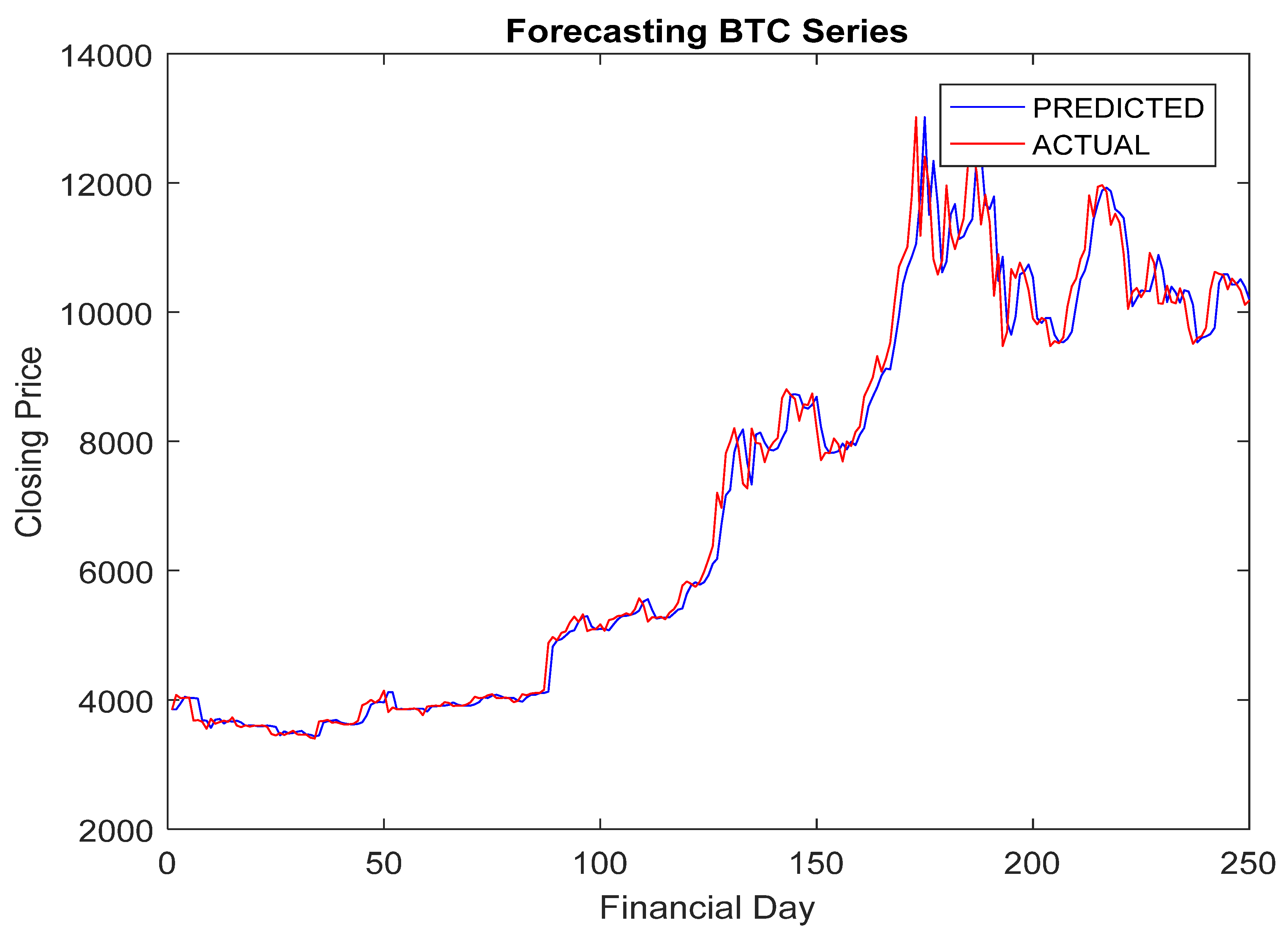
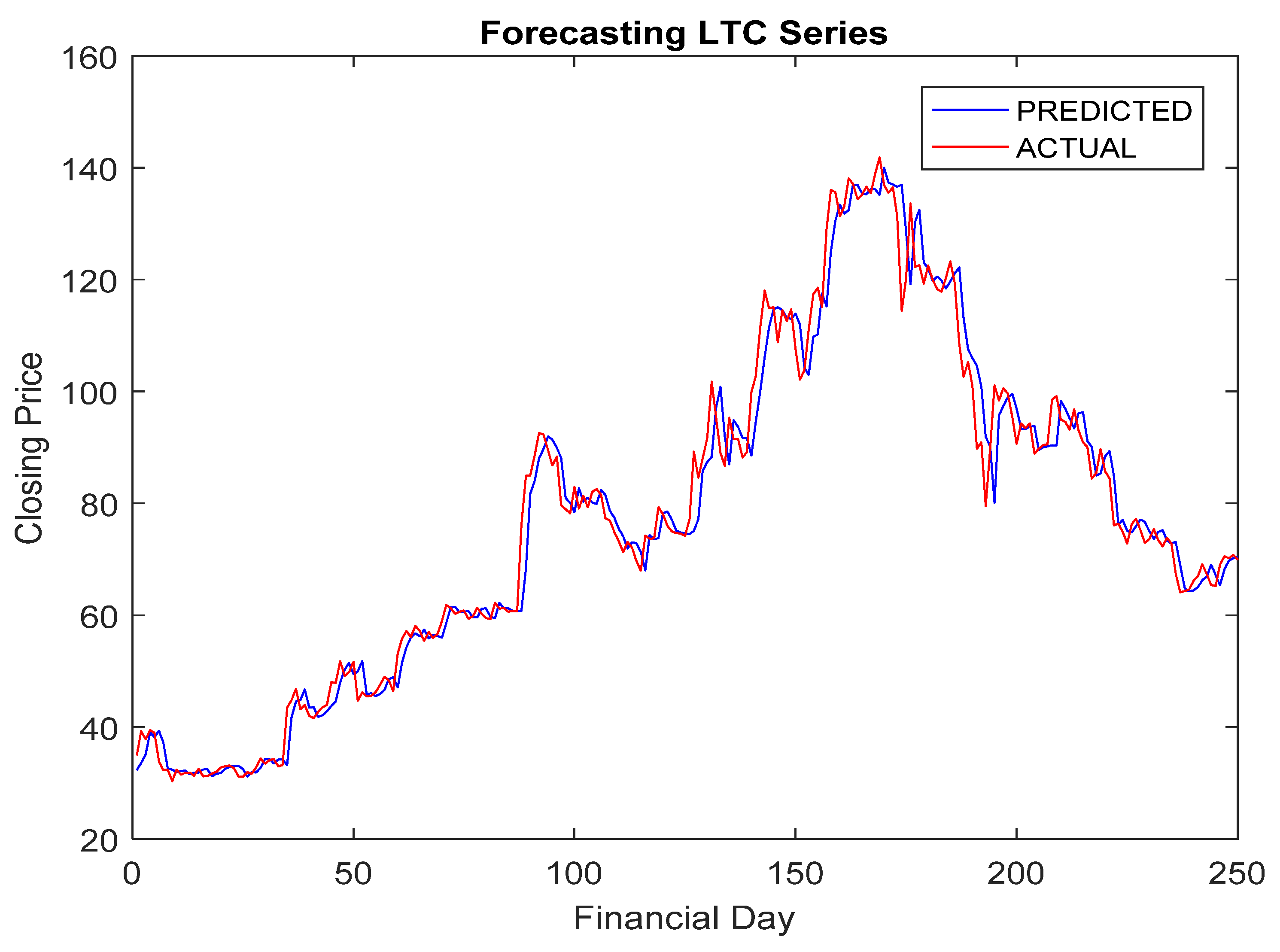
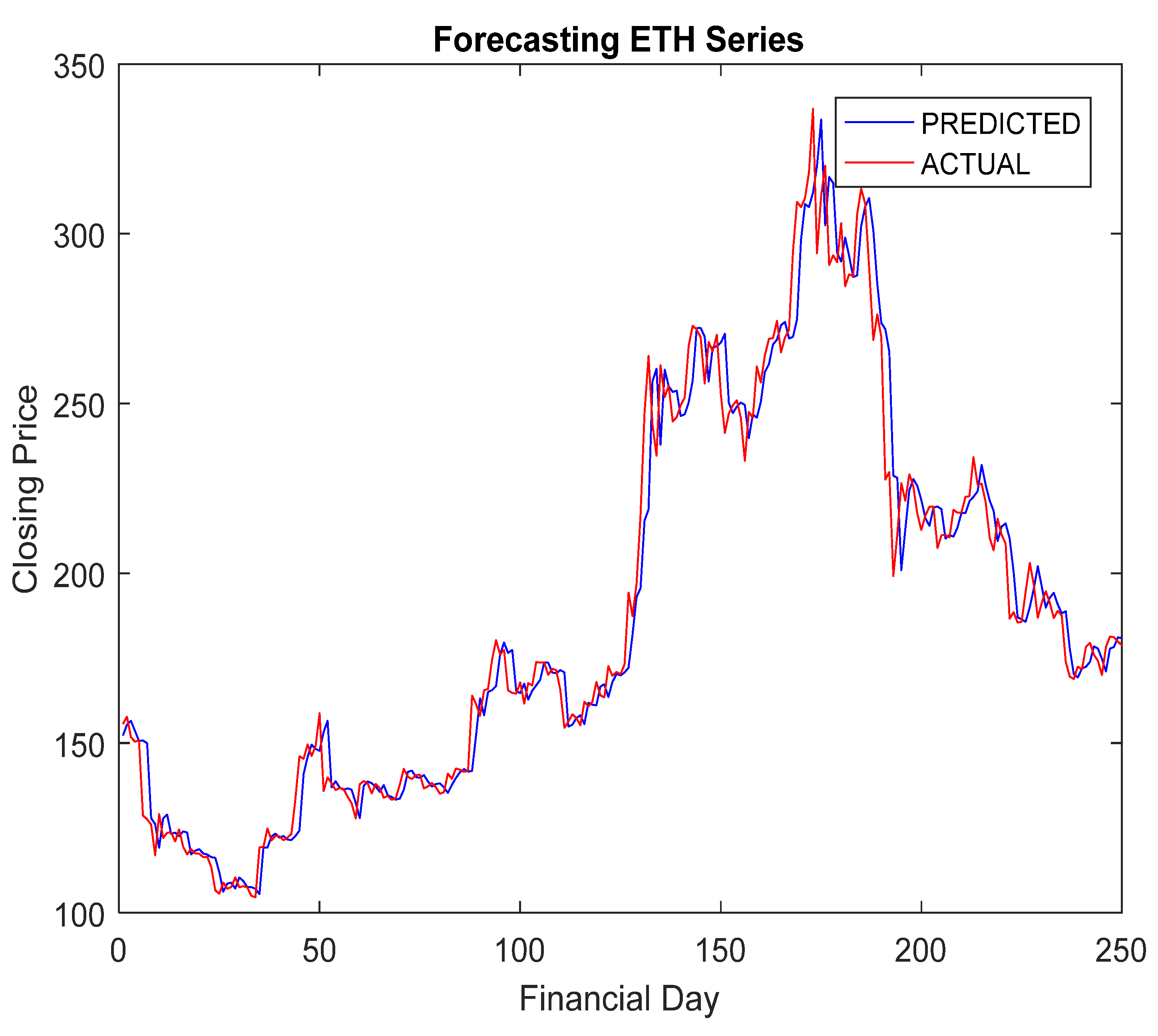
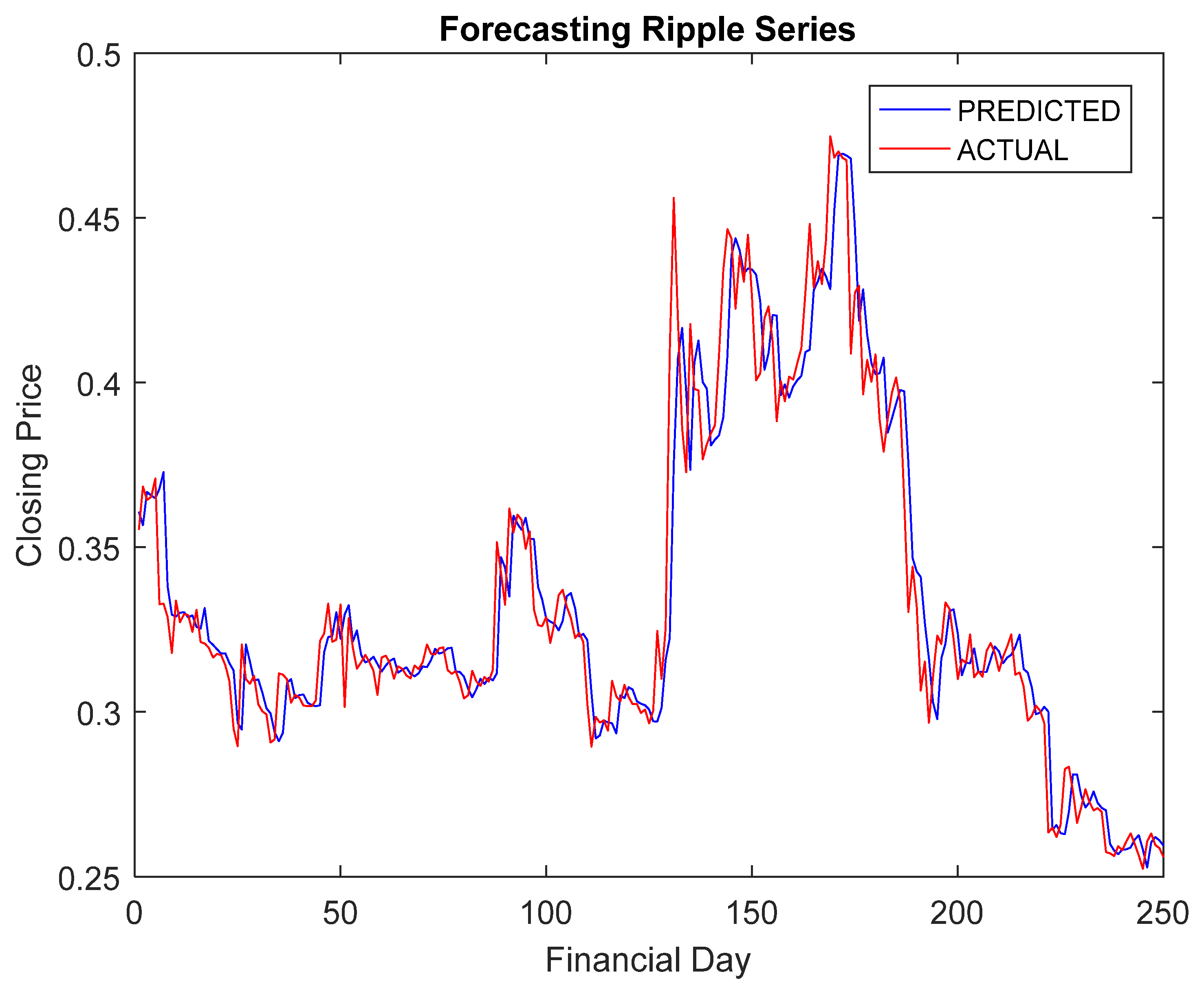
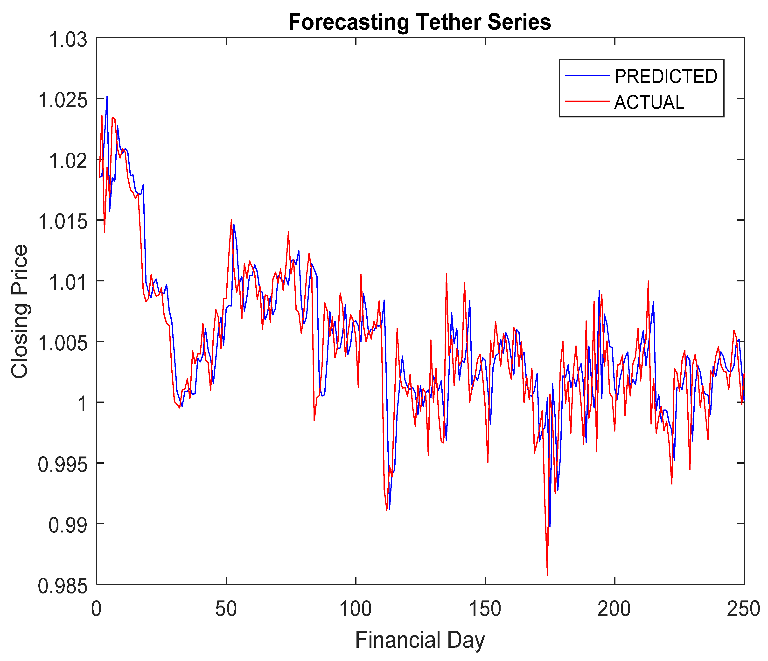
• The RA + ANN-based forecast was found quite capable in capturing the inherent dynamism and uncertainties associated with cryptocurrency data.
• The hybridization of RA and ANN achieved improved forecasting accuracy compared to others.
• The outcomes from the statistical test justified the significant difference between RA + ANN and others.

6. Conclusions

A hybrid ANN through Rao algorithm-based optimization (RA + ANN) is developed in this article using a single hidden layer ANN as the base neural architecture and RA as the search technique for exploiting the optimal ANN parameters. The Rao algorithms are recently proposed metaphor-less optimization techniques that are simple and do not need an algorithm-specific parameter to be adjusted. This article explored the modality of RA on training the ANN for forecasting cryptocurrency data such as Bitcoin, Litecoin, Ethereum, CMC 200, Tether, and Ripple. The RA + ANN predictability is compared with that of GA + ANN, PSO + ANN, MLP, SVM, ARIMA, and LSE in terms of MAPE and ARV. The proposed RA + ANN model has a faster convergence rate and better generalization ability compared to gradient descent learning. Furthermore, to ensure the effectiveness of RA + ANN, the Wilcoxon signed test and Diebold–Mariano test are conducted. From the comparative analysis of experimental results and outcomes of statistical significance tests, it is concluded that the RA + ANN-based forecasting is good enough to follow the dynamic trend of cryptocurrencies in comparison with the other forecasts under consideration. In the future, more ANN structures and sophisticated learning approaches may be investigated. Other factors such as the economic and technical determinants along with the closing prices may be used for achieving better forecasting accuracy. The proposed RA + ANN framework can also be applied for the efficient prediction of other existing FTS.

References

1. Lansky, J. Possible state approaches to cryptocurrencies. J. Syst. Integr. 2018, 9, 19–31. [Google Scholar] [CrossRef]
2. Nakamoto, S. Bitcoin: A peer-to-peer electronic cash system. Decentralized Bus. Rev. 2019, 21260. Available online: https://www.debr.io/article/21260.pdf (accessed on 26 March 2021).
3. Kyriazis, N.A. A survey on efficiency and profitable trading opportunities in cryptocurrency markets. J. Risk Financ. Manag. 2019, 12, 67. [Google Scholar] [CrossRef] [Green Version]
4. Mukhopadhyay, U.; Skjellum, A.; Hambolu, O.; Oakley, J.; Yu, L.; Brooks, R. A brief survey of cryptocurrency systems. In Proceedings of the 2016 14th annual conference on privacy, security and trust (PST), Auckland, New Zealand, 12–14 December 2016; pp. 745–752. [Google Scholar]
5. Ferreira, M.; Rodrigues, S.; Reis, C.I.; Maximiano, M. Blockchain: A tale of two applications. Appl. Sci. 2018, 8, 1506. [Google Scholar] [CrossRef] [Green Version]
6. Grinberg, R. Bitcoin: An innovative alternative digital currency. Hastings Sci. Technol. Law J. 2012, 4, 159. [Google Scholar]
7. Mai, F.; Shan, Z.; Bai, Q.; Wang, X.; Chiang, R.H. How does social media impact Bitcoin value? A test of the silent majority hypothesis. J. Manag. Inf. Syst. 2018, 35, 19–52. [Google Scholar] [CrossRef]
8. Sapuric, S.; Kokkinaki, A. Bitcoin Is Volatile! Isn’t That Right? Proceedings of the International Conference on Business Information Systems, Larnaca, Cyprus, 22–23 May 2014; Springer: Cham, Switzerland, 2014; pp. 255–265. [Google Scholar]
9. Corelli, A. Cryptocurrencies and exchange rates: A relationship and causality analysis. Risk 2018, 6, 111. [Google Scholar] [CrossRef] [Green Version]
10. Trabelsi, N. Are there any volatility spill-over effects among cryptocurrencies and widely traded asset classes? J. Risk Financ. Manag. 2018, 11, 66. [Google Scholar] [CrossRef] [Green Version]
11. Billah, M.; Waheed, S.; Hanifa, A. Stock market prediction using an improved training algorithm of neural network. In Proceedings of the 2016 2nd International Conference on Electrical, Computer & Telecommunication Engineering (ICECTE), Rajshahi, Bangladesh, 8–10 December 2016; pp. 1–4. [Google Scholar]
12. Nayak, S.C.; Misra, B.B.; Behera, H.S. An adaptive second order neural network with genetic-algorithm-based training (ASONN-GA) to forecast the closing prices of the stock market. Int. J. Appl. Metaheuristic Comput. (IJAMC) 2016, 7, 39–57. [Google Scholar] [CrossRef]
13. Nayak, S.C.; Misra, B.B.; Behera, H.S. Efficient forecasting of financial time-series data with virtual adaptive neuro-fuzzy inference system. Int. J. Bus. Forecast. Mark. Intelligence 2016, 2, 379–402. [Google Scholar] [CrossRef]
14. Rebane, J.; Karlsson, I.; Papapetrou, P.; Denic, S. Seq2Seq RNNs and ARIMA models for cryptocurrency prediction: A comparative study. In Proceedings of the SIGKDD Fintech’18, London, UK, 19–23 August 2018. [Google Scholar]
15. White, H. Economic prediction using neural networks: The case of IBM daily stock returns. In Proceedings of the IEEE 1988 International Conference on Neural Networks, San Diego, CA, USA, 24–27 July 1988; Volume 2, pp. 451–458. [Google Scholar]
16. Sureshkumar, K.K.; Elango, N.M. Performance analysis of stock price prediction using artificial neural network. Glob. J. Comput. Sci. Technol. 2012. [Google Scholar]
17. Misnik, A.; Krutalevich, S.; Prakapenka, S.; Borovykh, P.; Vasiliev, M. Impact Analysis of Additional Input Parameters on Neural Network Cryptocurrency Price Prediction. In Proceedings of the 2019 XXI International Conference Complex Systems: Control and Modeling Problems (CSCMP), Samara, Russia, 3–6 September 2019; pp. 163–167. [Google Scholar]
18. Jay, P.; Kalariya, V.; Parmar, P.; Tanwar, S.; Kumar, N.; Alazab, M. Stochastic neural networks for cryptocurrency price prediction. IEEE Access 2020, 8, 82804–82818. [Google Scholar] [CrossRef]
19. Akyildirim, E.; Goncu, A.; Sensoy, A. Prediction of cryptocurrency returns using machine learning. Ann. Oper. Res. 2020, 297, 3–36. [Google Scholar] [CrossRef]
20. Yazdinejad, A.; HaddadPajouh, H.; Dehghantanha, A.; Parizi, R.M.; Srivastava, G.; Chen, M.Y. Cryptocurrency malware hunting: A deep recurrent neural network approach. Appl. Soft Comput. 2020, 96, 106630. [Google Scholar] [CrossRef]
21. Alessandretti, L.; ElBahrawy, A.; Aiello, L.M.; Baronchelli, A. Anticipating cryptocurrency prices using machine learning. Complexity 2018, 2018, 8983590. [Google Scholar] [CrossRef]
22. Corbet, S.; Lucey, B.; Urquhart, A.; Yarovaya, L. Cryptocurrencies as a financial asset: A systematic analysis. Int. Rev. Financ. Anal. 2019, 62, 182–199. [Google Scholar] [CrossRef] [Green Version]
23. McNally, S.; Roche, J.; Caton, S. Predicting the price of bitcoin using machine learning. In Proceedings of the 2018 26th Euromicro International Conference on Parallel, Distributed and Network-Based Processing (PDP), Cambridge, UK, 21–23 March 2018; pp. 339–343. [Google Scholar]
24. Nakano, M.; Takahashi, A.; Takahashi, S. Bitcoin technical trading with artificial neural network. Phys. A Stat. Mech. Its Appl. 2018, 510, 587–609. [Google Scholar] [CrossRef]
25. Rao, R. Rao algorithms: Three metaphor-less simple algorithms for solving optimization problems. Int. J. Ind. Eng. Comput. 2020, 11, 107–130. [Google Scholar] [CrossRef]
26. Caesarendra, W.; Pratama, M.; Kosasih, B.; Tjahjowidodo, T.; Glowacz, A. Parsimonious network based on a fuzzy inference system (PANFIS) for time series feature prediction of low speed slew bearing prognosis. Appl. Sci. 2018, 8, 2656. [Google Scholar] [CrossRef] [Green Version]
27. Helfer, G.A.; Barbosa, J.L.; Alves, D.; da Costa, A.B.; Beko, M.; Leithardt, V.R. Multispectral cameras and machine learning integrated into portable devices as clay prediction technology. J. Sens. Actuator Netw. 2021, 10, 40. [Google Scholar] [CrossRef]
28. Alazeb, A.; Panda, B.; Almakdi, S.; Alshehri, M. Data Integrity Preservation Schemes in Smart Healthcare Systems That Use Fog Computing Distribution. Electronics 2021, 10, 1314. [Google Scholar] [CrossRef]
29. Nayak, S.C.; Misra, B.B.; Behera, H.S. On developing and performance evaluation of adaptive second order neural network with ga-based training (asonn-ga) for financial time series prediction. In Advancements in Applied Metaheuristic Computing; IGI Global: Hershey, PA, USA, 2018; pp. 231–263. [Google Scholar]
30. Nayak, S.C.; Misra, B.B.; Behera, H.S. Efficient financial time series prediction with evolutionary virtual data position exploration. Neural Comput. Appl. 2019, 31, 1053–1074. [Google Scholar] [CrossRef]
31. Mirjalili, S.; Mirjalili, S.M.; Hatamlou, A. Multi-verse optimizer: A nature-inspired algorithm for global optimization. Neural Comput. Appl. 2016, 27, 495–513. [Google Scholar] [CrossRef]
32. Nayak, S.C.; Das, S.; Misra, B.B. Development and Performance Analysis of Fireworks Algorithm-Trained Artificial Neural Network (FWANN): A Case Study on Financial Time Series Forecasting. In Handbook of Research on Fireworks Algorithms and Swarm Intelligence; IGI Global: Hershey, PA, USA, 2020; pp. 176–194. [Google Scholar]
33. Tan, Y.; Zhu, Y. Fireworks Algorithm for Optimization. In Proceedings of the International Conference in Swarm Intelligence, Beijing, China, 12–15 June 2010; Springer: Berlin, Germany, 2010; pp. 355–364. [Google Scholar]
34. Alatas, B. ACROA: Artificial chemical reaction optimization algorithm for global optimization. Expert Syst. Appl. 2011, 38, 13170–13180. [Google Scholar] [CrossRef]
35. Nayak, S.C.; Misra, B.B. A chemical-reaction-optimization-based neuro-fuzzy hybrid network for stock closing price prediction. Financ. Innov. 2019, 5, 38. [Google Scholar] [CrossRef]
36. Rao, R.V.; Savsani, V.J.; Vakharia, D.P. Teaching–learning-based optimization: An optimization method for continuous non-linear large scale problems. Inf. Sci. 2012, 183, 1–15. [Google Scholar] [CrossRef]
37. Rao, R. Jaya: A simple and new optimization algorithm for solving constrained and unconstrained optimization problems. Int. J. Ind. Eng. Comput. 2016, 7, 19–34. [Google Scholar]
38. Rao, R.V.; Pawar, R.B. Constrained design optimization of selected mechanical system components using Rao algorithms. Appl. Soft Comput. 2020, 89, 106141. [Google Scholar] [CrossRef]
39. Rao, R.V.; Pawar, R.B. Self-adaptive multi-population Rao algorithms for engineering design optimization. Appl. Artif. Intell. 2020, 34, 187–250. [Google Scholar] [CrossRef]
40. Premkumar, M.; Babu, T.S.; Umashankar, S.; Sowmya, R. A new metaphor-less algorithms for the photovoltaic cell parameter estimation. Optik 2020, 208, 164559. [Google Scholar] [CrossRef]
41. Wang, L.; Wang, Z.; Liang, H.; Huang, C. Parameter estimation of photovoltaic cell model with Rao-1 algorithm. Optik 2020, 210, 163846. [Google Scholar] [CrossRef]
42. Jabir, H.A.; Kamel, S.; Selim, A.; Jurado, F. Optimal Coordination of Overcurrent Relays Using Metaphor-less Simple Method. In Proceedings of the 2019 21st International Middle East Power Systems Conference (MEPCON), Cairo, Egypt, 17–19 December 2019; pp. 1063–1067. [Google Scholar]
43. Haykin, S. Neural Networks and Learning Machines 3/E; Pearson Educ: Delhi, India, 2010. [Google Scholar]
44. Nayak, S.C.; Misra, B.B.; Behera, H.S. Impact of data normalization on stock index forecasting. Int. J. Comput. Inf. Syst. Ind. Manag. Appl. 2014, 6, 257–269. [Google Scholar]
45. Nayak, S.C.; Misra, B.B. Extreme learning with chemical reaction optimization for stock volatility prediction. Financ. Innov. 2020, 6, 16. [Google Scholar] [CrossRef]
Figure 1. Basic Architecture of ANN. (Source: Authors).
Fintech 01 00004 g001
Figure 2. RA + ANN-based forecasting.
Fintech 01 00004 g002
Figure 3. Bitcoin, Litecoin, Ethereum, Ripple, CMC 200, and Tether FTSs.
Fintech 01 00004 g003
Figure 4. Rolling window method for input pattern generation.
Fintech 01 00004 g004
Figure 5. Forecasted prices v/s actual from Bitcoin.
Fintech 01 00004 g005
Figure 6. Forecasted prices v/s actual from Litecoin.
Fintech 01 00004 g006
Figure 7. Forecasted prices v/s actual from Ethereum.
Fintech 01 00004 g007
Figure 8. Forecasted prices v/s actual from Ripple.
Fintech 01 00004 g008
Figure 9. Forecasted prices v/s actual from CMC 200.
Fintech 01 00004 g009
Figure 10. Forecasted prices v/s actual from Tether.
Fintech 01 00004 g010