Improving Separation Prediction of Cyclone Separators with a Hybrid URANS-LES Turbulence Model

Abstract

The CFD simulation of cyclone separators has remarkably evolved over the past decades. Nowadays, computational models are essential for designing, analyzing, and optimizing these devices. Due to the intrinsic anisotropy of the flow inside these separators, the Reynolds stress model (RSM) has been mostly employed. However, RSM models fail to solve most time and space scales, including those relevant to particle behavior. Consequently, the prediction of the grade collection efficiency may be hindered, particularly for low-Stokes-number particles. For example, the precessing vortex core phenomenon (PVC), a well-known phenomenon that is relevant for particle motion, is not usually captured in Reynolds-averaged Navier–Stokes (RANS) simulations. Alternatively, the large-eddy simulation (LES) has been proven to be a superior approach since it captures many time and space scales that would have been otherwise dissipated, allowing for more accurate predictions of particle collection. However, this accuracy comes at a considerable computational cost. To combine the advantages of these two models, the main objective of this research was to evaluate a new hybrid RSM-LES model applied to the cyclone’s flow. The results were compared to experimental data and with RSM model results. It showed that, compared to a RANS model given by the RSM closure model, the grade collection efficiency curve obtained by the hybrid model is closer to the experimental one, even for the coarser mesh. Beyond that, the results showed that while the improvement in results was not proportional to mesh refinement for RANS modeling, the hybrid model showed significant improvement with mesh refinement.

1. Introduction

Cyclone separators are a crucial class of separation equipment with applications ranging from controlling emissions on Earth to removing dust from the atmosphere in Mars stations. Although their separation principle remains the same, i.e., the centrifugal field produced by the fluid motion, cyclones have been continually optimized due to advances in numerical techniques such as computational fluid dynamics (CFD) and hardware. As demonstrated in many works over the past decades [1,2,3,4,5,6,7,8], the anisotropic fluid flow within cyclones typically requires two-point turbulence closure models, such as the Reynolds stress model (RSM) or, alternatively, large-eddy simulation (LES), which is significantly more expensive. In their original formulation, RANS models, such as k-$\epsilon$ or SST, are incapable of simulating the Rankine vortex, which characterizes the flow within cyclone separators.

Gronald and Derksen [1] conducted simulations of the gas flow field in a cyclone separator using a RANS closure model and two LES approaches, one using finite volume and the other using lattice-Boltzmann discretization. The results were compared with experimental data from the literature, and the authors concluded that unsteady simulations using RANS and a relatively coarse grid can provide reasonable and industrially relevant results with low computational effort. A large-eddy approach with finer grids can reveal more of the flow physics but comes with a higher computational cost. Shukla et al. [3] used the RSM and large-eddy simulation to numerically evaluate the effect of velocity fluctuation modeling on the prediction of collection efficiency of cyclone separators. The simulated results were compared with experimental observations from the literature, showing that the LES has good performance in predicting the fluctuating flow field and collection efficiency for all particle sizes, while the performance of the RSM for these variables is poor, especially for small particles. Jang et al. [5] used the RSM and large-eddy simulation to investigate the flow field and collection efficiency of a Stairmand-type cyclone separator. The numerical results of mean velocity, pressure drop, and grade collection efficiency were compared with experimental data, showing that the LES yields results closer to the experimental ones for all the analyzed variables. Wasilewski et al. [6] evaluated the accuracy and reliability of two turbulence closure models, k-$\epsilon$ RNG and RSM (RANS), as well as LES, by comparing their outputs to experimental data in the analysis and characterization of multiphase flow phenomena inside the lower stage cyclone separator used in the clinker burning process. The obtained results showed that, for this case, the LES model proved to be the most accurate in forecasting the separation efficiency and pressure drop. The RSM model also achieved high accuracy, but the k-$\epsilon$ RNG model was characterized by significantly larger deviations.

While some of the aforementioned studies reported satisfactory outcomes through the use of RSM, one notable drawback of RANS models is their inherent tendency to yield average flow fields, regardless of mesh resolution. Given the considerable advancements in hardware technology over recent decades, performing simulations on fine grids is now within reach of personal computers. Consequently, it would be advantageous to develop turbulence closure techniques that can automatically switch between RANS and LES models. This approach would allow for the advantages of two different approaches: swift, average computations for coarse grids and more precise, scale-resolving calculations for finer grids.

Indeed, the reasoning behind DES (detached-eddy simulation), PANS (partially averaged Navier–Stokes), and other hybrid models is that they provide a seamless transition between a RANS model (SST, SA, or k-$\epsilon$) and a one- or two-equation LES model [9,10,11,12,13]. These approaches, based mainly on local mesh metrics, allow for the optimization of accuracy in a CFD computation for a given grid, which is dependent on available resources. While a RANS calculation yields no increase in accuracy beyond mesh-independence resolution, these hybrid approaches produce results approaching LES with greater grid refinement.

To the best of the authors’ knowledge, no hybrid model involving the RSM has been proposed yet. This would mostly hinder the use of hybrid approaches for cyclones with strong swirl. The aim of this work is to suggest such a new model and exhibit its application. The innovative model retrieves the RSM model in the near-wall regions, where LES mesh requirements are typically very high, while generating less dissipation in regions where the LES mesh criteria are fulfilled. The model’s performance is evaluated in a particularly demanding setup that encompasses a small-diameter cyclone (and thus, a strongly swirling flow field) and very low-Stokes-number particles. Previous LES findings [2,14,15] for the same geometry suggested that mesh resolutions in the order of 1 million hexahedra were necessary for an accurate prediction of the collection efficiency.

The novel model is expounded in Section 2.2.2, and its implementation can be made in any commercial or open-source software. The outcomes for the collection efficiency are juxtaposed to those produced by the conventional RSM model, and the precision is elevated for the equivalent grid. The precision is also enhanced in comparison to the antecedent outcomes utilizing the LES model [2,14,15]. The discoveries are highly promising and suggest that the model can be utilized in other problems that entail particles in swirling flow fields.

2. Materials and Methods

2.1. Solution Setup

To evaluate the hybrid model proposed in the present paper and to compare it with the RSM results, experimental data from Xiang et al. [16] were used. The geometry is illustrated in the Figure 1 and the dimensions are presented in

Table 1. Cyclone dimensions [16].

Dimension	Length (mm)
Body diameter (Dc)	31
Gas outlet diameter (De)	15.5
Inlet height (a)	12.5
Inlet width (b)	5
Cyclone height (H)	77
Cylinder height (h)	31
Gas outlet duct length (S)	15.5
Cone bottom opening (B)	19.4

.

The simulations were carried out in two phases. The fluid phase consists of air, with a density of 1.205 kg/m³ and a viscosity of 1.82 $\times {10}^{-5}$ kg/m.s. The imposed inlet velocities were 8 m/s, 10.67 m/s, and 13.33 m/s, which led to Reynolds numbers of 16,420; 21,900; and 27,360, respectively, which characterizes turbulent flows.

As for the disperse phase, particles with a density of 1050 kg/m${}^3$ were injected at the same velocity as the fluid, with a mass flow rate of 0.000275 kg/s. The first time step involved injecting 96,000 particles, with 8000 of each diameter ranging between 0.5 $\mathsf{\mu }$m and 6 $\mathsf{\mu }$m. It was assumed that the particles would reflect when colliding with the wall, escape when crossing the overflow, and be collected when touching the underflow.

The physical assumptions behind the CFD model are sumarized in

Table 2. Physical assumptions of the CFD model.

Characteristics	Assumptions
Density	Constant (incompressibility)
Viscosity	Newtonian Fluid
Gravity	9.81 $\mathrm{m}/{\mathrm{s}}^2$
Turbulence	Fully Turbulent RSM
	Fully Turbulent hybrid URANS-LES
Thermal efects	Neglected

, and the setup details are shown in

Table 3. Setup definition.

Characteristics	Value/Description
Fluid density	1.205 kg/m${}^3$
Disperse phase density	1050 kg/m${}^3$
Fluid inlet velocity	8 m/s
	10.67 m/s
	13.33 m/s
Disperse phase inlet velocity	Same as the fluid
Fluid viscosity	1.82 $\times {10}^{-5}$ kg/m.s
Disperse phase mass flow rate	0.000275 kg/s
Time step	0.0001 s
Time scheme	Three-level implicit
Advective scheme	Second-order upwind
Diffusive scheme	Second order centered difference
Disperse phase coupling	One-way
Disperse phase modeling	Lagrangian approach
Convergence criteria	1 $\times {10}^{-4}$
Pressure–velocity coupling	SIMPLE

. The unsteady simulations were stopped once the number of particles inside the cyclone was less than 200.

The computational domain is a 3D cyclone with the dimensions showed in Table 1, as shown in Figure 2. The boundary conditions for the flow and for the particles are also shown in Figure 2. A uniform velocity inlet boundary is prescribed at the inlet surface of the cyclone. A pressure outlet boundary is applied at the overflow and particles are allowed to escape through this boundary. For the collection criteria, the underflow outlet is defined as a wall, so the particles that touch it are considered collected. No-slip boundary conditions are imposed at all the other surfaces.

Unstructured grids are generated using the ICEM software. As can be seen in Figure 2, the grids near the walls have a higher grid-node density. To evaluate the effect of the grid refinement, three meshes consisting of nearly 180,000; 400,000; and 800,000 hexaedra were used. The mesh details are shown in Figure 3, Figure 4 and Figure 5 and in

Table 4. Mesh details.

Mesh	Number of Cells	Typical y+	Min. Volume (${\mathbf{m}}^3$)	Max. Volume (${\mathbf{m}}^3$)
Coarse	195,522	1.7	1.24673 $\times {10}^{-11}$	1.74645 $\times {10}^{-9}$
Medium	426,486	0.85	5.95138 $\times {10}^{-12}$	1.79744 $\times {10}^{-9}$
Fine	838,544	0.85	4.71827 $\times {10}^{-12}$	5.74385 $\times {10}^{-10}$

.

2.2. Mathematical Model

In this paper, two turbulence closure models were employed: the RSM and the hybrid model. These two models, along with the model used for the dispersed phase, are presented in this section.

The numerical solution of the equations presented in this section was performed using the computational code UNSCYFL3D. This in-house software is based on the finite volume method on unstructured three-dimensional grids. In all simulations conducted in this study, the three-time-level scheme was utilized for time advancement, the centered differencing scheme was employed for the diffusive term of the momentum equations, and the second-order upwind scheme was used for the advective term of the momentum equations. The SIMPLE (semi-implicit method for pressure-linked equations) algorithm was used to couple the velocity and pressure fields.

2.2.1. RSM Model

In the Reynolds stress model, the equations for each component of Reynolds stress are derived by filtering the Navier–Stokes equations, resulting in

$$\begin{array}{c}\hfill \frac{\partial \left(\rho \overline{{u_i}^{\prime }{u_j}^{\prime }}\right)}{\partial t}=-\frac{\partial \left(\rho \overline{{u_k}^{\prime }{u_i}^{\prime }{u_j}^{\prime }}\right)}{\partial x_k}-\frac{\partial }{\partial x_k}\left[\rho \overline{{u_i}^{\prime }{u_j}^{\prime }{u_k}^{\prime }}+\overline{p\left({\delta }_{kj}{u}_i^{\prime }+{\delta }_{ik}{u}_j^{\prime }\right)}\right]+\frac{\partial }{\partial x_k}\left[\mu \left(\frac{\partial \overline{{u_i}^{\prime }{u_j}^{\prime }}}{\partial x_k}\right)\right]\\ \hfill -\rho \left(\overline{{u_i}^{\prime }{u_k}^{\prime }}\frac{\partial \overline{u_j}}{\partial x_k}+\overline{{u_j}^{\prime }{u_k}^{\prime }}\frac{\partial \overline{u_i}}{\partial x_k}\right)+\overline{p\left(\frac{\partial u_i^{\prime }}{\partial x_j}+\frac{\partial u_j^{\prime }}{\partial x_i}\right)}-2\mu \overline{\frac{\partial u_i^{\prime }}{\partial x_k}\frac{\partial u_j^{\prime }}{\partial x_k}}\end{array}$$

(1)

where $\overline{{u_i}^{\prime }{u_j}^{\prime }}$ is the Reynolds stress, $\rho$ is the density, p is the pressure, $\delta$ is the Kronecker tensor, $\mathsf{\mu }$ is the viscosity, $u_i$ are the velocity components, and $x_i$ are the position components. Some terms in Equation (1) require modeling, resulting in

$$\begin{array}{c}\hfill \frac{\partial \left(\rho \overline{{u_i}^{\prime }{u_j}^{\prime }}\right)}{\partial t}=-\frac{\partial \left(\rho \overline{{u_k}^{\prime }{u_i}^{\prime }{u_j}^{\prime }}\right)}{\partial x_k}-\frac{\partial }{\partial x_k}\left[\frac{{\mu }_t}{{\sigma }_k}\left(\frac{\partial \overline{u_i^{\prime }{u}_j^{\prime }}}{\partial x_k}\right)\right]+\frac{\partial }{\partial x_k}\left[\mu \left(\frac{\partial \overline{{u_i}^{\prime }{u_j}^{\prime }}}{\partial x_k}\right)\right]\\ \hfill -\rho \left(\overline{{u_i}^{\prime }{u_k}^{\prime }}\frac{\partial \overline{u_j}}{\partial x_k}+\overline{{u_j}^{\prime }{u_k}^{\prime }}\frac{\partial \overline{u_i}}{\partial x_k}\right)+{\varphi }_{ij,1}+{\varphi }_{ij,2}+{\varphi }_{ij,3}-\epsilon \end{array}$$

(2)

where

$${\varphi }_{ij,1}=-C_1\frac{\epsilon }{k}\left(\overline{u_i^{\prime }{u}_j^{\prime }}-\frac{2}{3}{\delta }_{ij}k\right)$$

(3)

$${\varphi }_{ij,2}=-C_2\left[(P_{ij}-A_{ij})-\frac{2}{3}{\delta }_{ij}{P}_{ij}\right]$$

(4)

$$\begin{array}{c}\hfill {\varphi }_{ij,3}=C_{1,w}\frac{\epsilon }{k}\left(\overline{u_k^{\prime }{u}_m^{\prime }}{n}_k{n}_m{\delta }_{ij}-\frac{3}{2}\overline{u_i^{\prime }{u}_k^{\prime }}{n}_j{n}_k-\frac{3}{2}\overline{u_j^{\prime }{u}_k^{\prime }}{n}_i{n}_k\right)\frac{k^{\frac{3}{2}}}{C_l\epsilon d}\\ \hfill +C_{2,w}\left({\varphi }_{km,2}{n}_k{n}_m{\delta }_{ij}-\frac{3}{2}{\varphi }_{ik,2}{n}_j{n}_k-\frac{3}{2}{\varphi }_{jk,2}{n}_i{n}_k\right)\frac{k^{\frac{3}{2}}}{C_l\epsilon d}\end{array}$$

(5)

$$\frac{\partial \left(\rho \epsilon \right)}{\partial t}+\frac{\partial \left(\rho \epsilon u_i\right)}{\partial x_i}=\frac{\partial }{\partial x_j}\left[\left(\mu +\frac{{\mu }_t}{{\sigma }_{\epsilon }}\right)\frac{\partial k}{\partial x_j}\right]+\frac{C_{\epsilon 1}\epsilon P_{ii}}{2k}-\frac{C_{\epsilon 2}\rho {\epsilon }^2}{k}$$

(6)

$\epsilon$ is the turbulent dissipation, k is the turbulent kinetic energy, $P_{ij}$ is the transformation term, $A_{ij}$ is the advective term, $n_k$ is the vector unit normal to the wall $x_k$, and d is the distance to the wall. $C_1,C_2,C_{1,w}$ e $C_{2,w}$ are empirical constants, and $C_l$ is 0.39. $C_{\epsilon 1}$ and $C_{\epsilon 2}$ are 1.2, ${\sigma }_k$ is 0.82, and ${\sigma }_{\epsilon }$ is 1.

2.2.2. Hybrid LES-RSM Model

The hybrid model proposed in the present paper is founded upon the research by Hadžiabdic and Hanjalic [9]. It employs a grid detection parameter, $\alpha$, which is incorporated into the RSM (Equation (1)). This results in decreased dissipation in regions where the mesh is adequately refined and more turbulent scales are resolved. The relevant equations are as follows:

$$\begin{array}{c}\hfill \frac{\partial \left(\rho \overline{{u_i}^{\prime }{u_j}^{\prime }}\right)}{\partial t}=-\frac{\partial \left(\rho \overline{{u_k}^{\prime }{u_i}^{\prime }{u_j}^{\prime }}\right)}{\partial x_k}-\frac{\partial }{\partial x_k}\left[\frac{{\mu }_t}{{\sigma }_k}\left(\frac{\partial \overline{u_i^{\prime }{u}_j^{\prime }}}{\partial x_k}\right)\right]+\frac{\partial }{\partial x_k}\left[\mu \left(\frac{\partial \overline{{u_i}^{\prime }{u_j}^{\prime }}}{\partial x_k}\right)\right]\\ \hfill -\rho \left(\overline{{u_i}^{\prime }{u_k}^{\prime }}\frac{\partial \overline{u_j}}{\partial x_k}+\overline{{u_j}^{\prime }{u_k}^{\prime }}\frac{\partial \overline{u_i}}{\partial x_k}\right)+{\varphi }_{ij,1}+{\varphi }_{ij,2}+{\varphi }_{ij,3}-\alpha \epsilon \end{array}$$

(7)

$${\varphi }_{ij,1}=-C_1\frac{\alpha \epsilon }{k}\left(\overline{u_i^{\prime }{u}_j^{\prime }}-\frac{2}{3}{\delta }_{ij}k\right)$$

(8)

$${\varphi }_{ij,2}=-C_2\left[(P_{ij}-A_{ij})-\frac{2}{3}{\delta }_{ij}{P}_{ij}\right]$$

(9)

$$\begin{array}{c}\hfill {\varphi }_{ij,3}=C_{1,w}\frac{\alpha \epsilon }{k}\left(\overline{u_k^{\prime }{u}_m^{\prime }}{n}_k{n}_m{\delta }_{ij}-\frac{3}{2}\overline{u_i^{\prime }{u}_k^{\prime }}{n}_j{n}_k-\frac{3}{2}\overline{u_j^{\prime }{u}_k^{\prime }}{n}_i{n}_k\right)\frac{k^{\frac{3}{2}}}{C_l\alpha \epsilon d}\\ \hfill +C_{2,w}\left({\varphi }_{km,2}{n}_k{n}_m{\delta }_{ij}-\frac{3}{2}{\varphi }_{ik,2}{n}_j{n}_k-\frac{3}{2}{\varphi }_{jk,2}{n}_i{n}_k\right)\frac{k^{\frac{3}{2}}}{C_l\alpha \epsilon d}\end{array}$$

(10)

The grid detecting parameter is obtained from

$$\alpha =max\left(1,\frac{L_{RANS}}{L_{LES}}\right)$$

(11)

where

$$L_{RANS}=\frac{k^{1.5}}{\epsilon }$$

(12)

$$L_{LES}=C_{\Delta }{(\Delta V)}^{1/3}$$

(13)

where k is the modeled turbulent kinetic energy and $C_{\Delta }$ is the filtering constant.

To behave like a hybrid model incorporating LES in the outer flow region, the parameter $\alpha$ modifies the implicit characteristic turbulence length scale from $L_{RANS}$ (RANS) to the subgrid-scale from LES. The model also applies a switching criterion to determine the turbulent viscosity between both the models.

$${\nu }_t=max({\nu }_t^{RANS},{\nu }_t^{LES})$$

(14)

Then, in close proximity to the wall, $\alpha$ equals the unitary value and the closure model works similarly to RANS framework. As the distance from the wall increases, $L_{RANS}>L_{LES}$ and $\alpha >1$, which decrases ${\nu }_t^{RANS}$.

As $\alpha$ becomes greater than 1, the energy stored in the resolved scales increases. Therefore, in order to calculate $L_{RANS}$, the total turbulent kinetic energy ($k_{tot}$) must be taken into account, which is obtained by adding the resolved ($k_{res}$) and modeled ($k_{mod}$) parts. Equation (12) is then rewritten as:

$$L_{RANS}=\frac{k_{tot}^{1.5}}{\epsilon }=\frac{{(k_{res}+k_{mod})}^{1.5}}{\epsilon }$$

(15)

2.2.3. Dispersed Phase Modeling

The dispersed phase is modeled using a Lagrangian framework, whereby each particle is tracked through the domain and its motion is governed by Newton’s second law. The relevant equations are as follows:

$$\frac{d{x}_{pi}}{dt}=u_{pi}$$

(16)

$$m_p\frac{d{u}_{pi}}{dt}=m_p\frac{3\rho C_D}{4{\rho }_p{d}_p}(u_i-u_{pi})+\left(1-\frac{\rho }{{\rho }_p}\right)m_p{g}_i$$

(17)

$$I_p\frac{d{\omega }_{pi}}{dt}=T_i$$

(18)

where $d_p$ is the particle diameter, $m_p$ is the particle mass, and $I_p$ is the moment of inertia for an espherical particle. To calculate the drag coefficient ($C_D$), the correlation of Shiller and Naumann [17] presented below is employed.

$$C_D=\left\{\begin{array}{c}24R{e}_p^{-1}\left(1+0.15R{e}_p^{0.687}\right)\mathrm{if}R{e}_p\le 1000\\ 0.44\mathrm{if}R{e}_p>1000\end{array}\right.$$

(19)

$$R{e}_p=\frac{\rho d_p|\overrightarrow{u}-{\overrightarrow{u}}_p|}{\mu }$$

(20)

One final equation is required to calculate the torque ($T_i$) mentioned in Equation (18). This equation is

$$\overrightarrow{T}=C_r\frac{\rho d_p^5}{64}\left|\overrightarrow{\mathsf{\Omega }}\right|\overrightarrow{\mathsf{\Omega }}$$

(21)

where

$$C_r=\left\{\begin{array}{c}\frac{64\pi }{R{e}_r}\mathrm{if}R{e}_r\le 32\\ \frac{12.9}{\sqrt{R{e}_r}}+\frac{128.4}{R{e}_r}\mathrm{if}R{e}_r>32\end{array}\right.$$

(22)

In Equation (17) forces such as Saffman’s, Basset and virtual force have been neglected. This is feasible in the present case since the material density of the particle is almost 1000 times that of the gas [18,19].

3. Results and Discussions

3.1. Velocity Profiles

Three different cases varying the inlet flow rate, and therefore the Reynolds number, were run, i.e., 16,420; 21,900; and 27,360. As the Reynolds numbers are close to each other, the analysis of the velocity profiles will only be performed for the intermediate value, as its behavior can be extended to the other two flow rates. The velocity profile was computed at a center-line positioned at 0.05 m on a plane positioned in the X-section at the center of the cyclone. It is worth noting here the importance of presenting mesh tests throughout the results. Since hybrid modeling has the potential for improvement over the RANS model in its ability to calculate a wider range of scales as the mesh is refined. It is expected that the greatest difference between both methods occurs for more refined meshes.

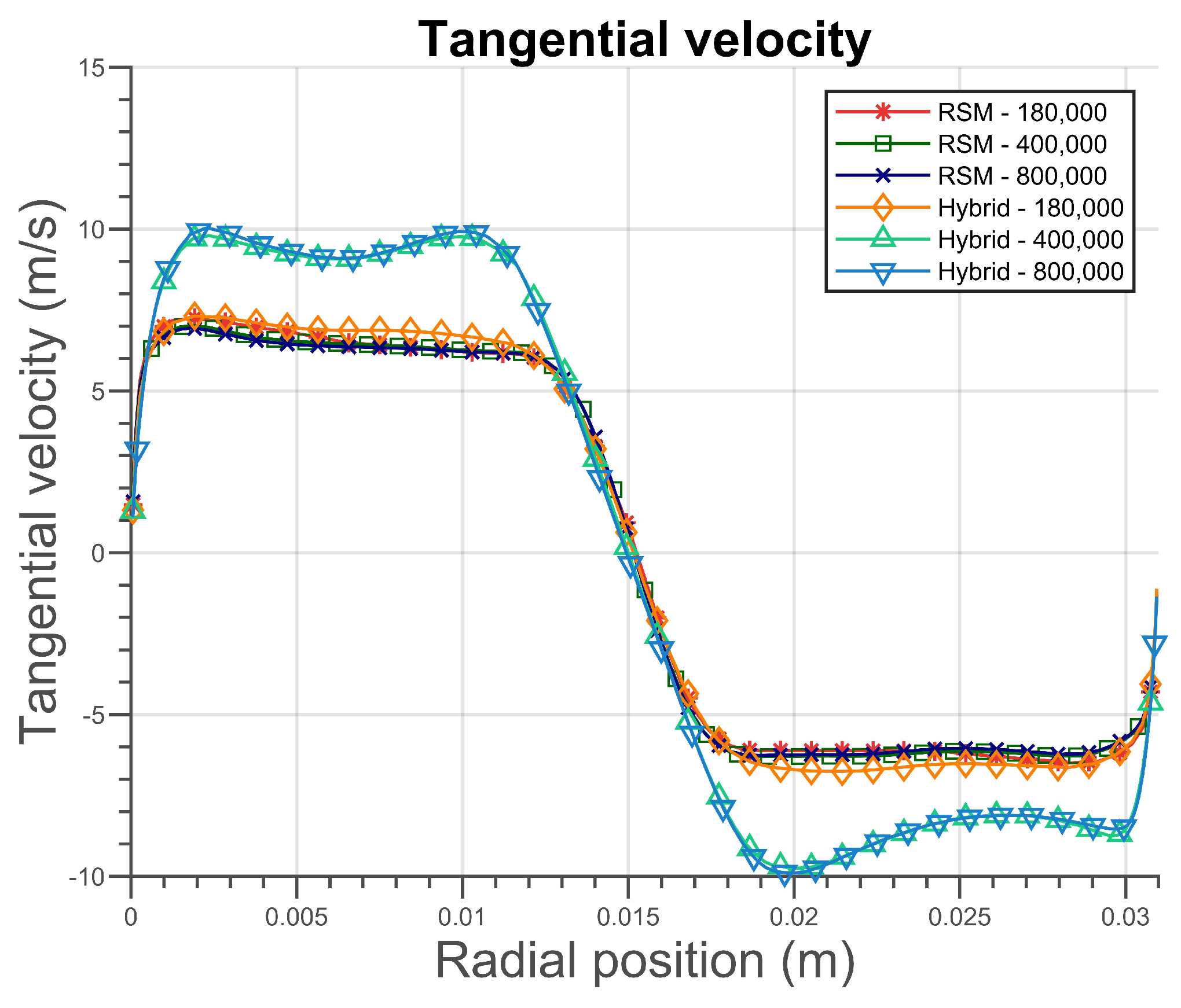
Figure 6 displays the tangential velocity profile for the three different meshes, named mesh 1, 2, and 3; i.e., 180,000; 400,000; and 800,000 volumes each, respectively, and the two different models employed in the present study, RSM and the hybrid model. It is evident that, in all cases, the tangential velocity profile exhibits positive values on the left side and negative values on the right side, indicating the rotational motion around the central axis, as anticipated.

Results from the RSM and the hybrid model are quite similar for the coarsest mesh; however, regarding meshes 2 and 3, there is a more pronounced difference between the closure models. For instance, the peak values for RANS are approximately 7 m/s, whereas for the hybrid modeling, they vary around 9.5 m/s. This discrepancy can be explained by the fact that the coarser grid is not refined enough to enable the hybrid model to employ the LES model extensively in the domain, resulting in the hybrid model working almost like the RSM.

Regarding the differences between the meshes employing the RSM, it can be noted that the velocity profiles are quite similar, demonstrating that improvement in results is not proportional to the mesh refinement for RANS modeling, since the filtering of temporal scales in this type of closure model is given by the mean operator and not a filter dependent on the calculated scales. However for the hybrid model, only meshes 2 and 3 were consistent, whereas the 180,000 grid yielded a lower result. This mainly indicates that for the RSM model, grid independence was attained, so increasing the refinement does not generate significant differences in the results. However, for the hybrid model, the coarser mesh does not enable the extensive use of the LES scheme in the domain, while the two most refined meshes allow it.

Figure 7 illustrates the variations of the RMS velocity along the analysis line, which indicates the fluctuations in the flow velocity field. It can be noted that the hybrid model generated higher values of RMS velocity than the RSM model, as expected since the RSM model models the mean velocity, while the hybrid model uses the LES in some regions, calculating a wider spectrum of velocity scales.

Figure 8 presents a similar analysis for the axial velocity component. Negative velocity values are found in the proximity of the walls. However, when the distance grows and the geometry center is approached, the velocity profile tends to rise and become positive, displaying an inverted W profile, as expected. The behavior of all six cases was analogous to that observed for the tangential velocity. With regard to the RSM, depicted in Figure 9, the generated meshes yielded nearly identical results, while the hybrid model produced notably dissimilar results for the coarser mesh. Additionally, the hybrid model’s results were distant from the RSM for meshes consisting of 400,000 and 800,000 cells, whereas the mesh composed of 180,000 hexahedral cells generated similar outcomes in both models.

3.2. Turbulent Kinetic Energy

The decomposition of turbulent kinetic energy (TKE) into modeled and resolved parts is significant in illustrating the concepts underlying the employed models. To analyze this parameter, only the most refined mesh (mesh 3) was used. On this basis, it is expected that the energy in the resolved scales will be higher and the LES closure model will be active in a larger portion of the domain. This highlights the significant differences between the RANS and hybrid methodologies. The TKE contour was extracted from the vertical plane cutting through the cyclone and passing through its center.

It is well known that the hybrid model employs LES in some regions of the domain, which solves equations for the large scales and models the subgrid-scales. In addition, the RSM model is known for modeling nearly all turbulent scales. In this regard, Figure 10 and Figure 11 display the TKE fields for the modeled and resolved scales, respectively, for both methodologies. For the hybrid model, the modeled portion only exhibits high values close to the wall, where $\alpha \to 1$ and the RSM is employed. In the outer flow region, the modeled portion is close to zero, indicating that only a few scales are modeled, while the resolved part demonstrates high values, indicating that most scales are resolved. In the pure RSM model (RANS), the modeled portion is high throughout the domain, and the resolved part is non-zero only in a small region at the gas outlet duct, demonstrating that this model models nearly all turbulent scales.

3.3. Collection Efficiency

The particle collection efficiency depicts the impact of numerical models and grid refinement on particle motion calculation. To examine this variable, the numerical results of the current paper were compared with experimental data from Xiang et al. [16]. To determine the collected particles, the underflow was defined as a wall, and all the particles that touched it were considered as collected.

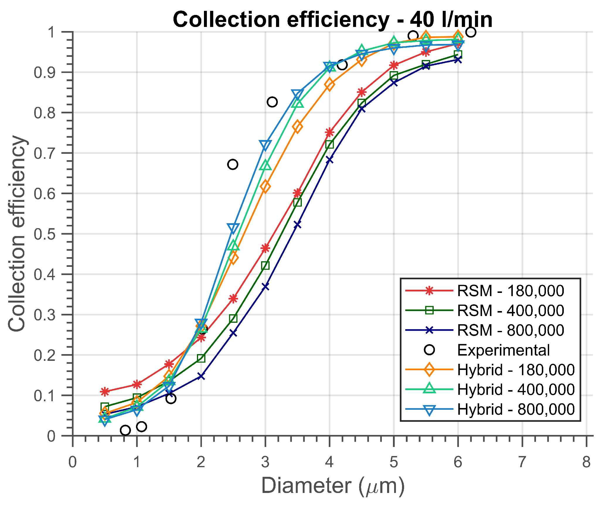
Figure 12, Figure 13 and Figure 14 exhibit the variation in the collection efficiency for the three flow rates studied, namely 30, 40, and 50 l/min, respectively. Each figure displays six S-shaped curves with computed values from the two studied closure models for the three examined meshes.

Table 5. Collection efficiency results for 30 l/min.

Flow Rate	30 l/min
Diameter  ($\mathsf{\mu }$m)	Exp.	Mesh	RSM	Hybrid
1	0.0033	Coarse	0.0975	0.0585
		Medium	0.0815	0.0645
		Fine	0.0724	0.0454
3	0.4918	Coarse	0.2846	0.3702
		Medium	0.2855	0.4787
		Fine	0.2562	0.46
6	0.9422	Coarse	0.8564	0.9549
		Medium	0.8451	0.9439
		Fine	0.8455	0.9295

,

Table 6. Collection efficiency results for 40 l/min.

Flow Rate	40 l/min
Diameter  ($\mathsf{\mu }$m)	Exp.	Mesh	RSM	Hybrid
1	0.0200	Coarse	0.1270	0.0826
		Medium	0.0944	0.0716
		Fine	0.0717	0.0647
3	0.7993	Coarse	0.4642	0.6172
		Medium	0.4214	0.6670
		Fine	0.3692	0.7219
6	0.9971	Coarse	0.9707	0.9875
		Medium	0.9436	0.9809
		Fine	0.9312	0.9686

and

Table 7. Collection efficiency results for 50 l/min.

Flow Rate	50 l/min
Diameter  ($\mathsf{\mu }$m)	Exp.	Mesh	RSM	Hybrid
1	0.0250	Coarse	0.1535	0.1189
		Medium	0.1131	0.0811
		Fine	0.0924	0.1076
3	0.9530	Coarse	0.6502	0.8047
		Medium	0.6034	0.8191
		Fine	0.5732	0.8628
6	0.9987	Coarse	0.9912	0.9935
		Medium	0.9757	0.9922
		Fine	0.9600	0.9801

show a comparision between the experimental result and the predictions from the RSM and hybrid models with the three different meshes for a small, a medium, and a high particle diameter.

Regarding the differences between the turbulence models, the results for the hybrid model are noticeably close to the experimental data, as can be shown. For small particles, that is, for diameters less than 1.5 $\mathsf{\mu }$m, it is evidenced that all models predict values higher than the experimental ones. However, as the particles increase in size, the models tend to exhibit divergent results. Furthermore, there is a reversal of behavior, and the numerical values for collection efficiency become lower than the data from Xiang et al. [16].

Once again, the hybrid model was the one that most closely approximated the expected results across the entire particle size range, particularly for medium sizes. This fact can be explained by the sensitivity of particles to small-wavelength fluctuations, as these fluctuations are taken into account only in the regions where LES is applied. That is, in the wall regions, the two models exhibit similar behaviors, and in the outer parts, for the hybrid model, the particles experience velocity fluctuation effects. This does not occur for the RANS modeling.

Moreover, the hybrid model reached higher velocity values, as demonstrated in the velocity profiles, which generated greater centrifugal force on the particles. This caused more particles to be carried to the wall and, consequently, to the underflow, increasing the collection efficiency. However, a higher velocity increases turbulence, which causes the reentrainment of particles that would otherwise be collected and disturbs the separation efficiency, as shown by Souza et al. [2]. The combination of these factors caused an increase in the collection efficiency calculated by the hybrid model compared to the RSM.

Regarding the influence of the mesh refinement, for a flow rate of 30 l/min, all results for the RSM model were very close to each other, especially for diameters greater than 4 $\mathsf{\mu }$m. For the hybrid model, the results for mesh 1 deviated from those acquired using the 400,000 and 800,000 cells, which demonstrated high similarity to each other and the experimental data. This pattern was also presented in the velocity field, where values from the two finer meshes closely resembled each other and substantially diverged from the coarser mesh data. For flow rates of 40 l/min and 50 l/min, a larger discrepancy existed between the RSM model’s results with the three meshes. This suggested that minor variations in fluid flow significantly impacted particle motion. Regarding the hybrid model, it was observed that the values obtained for meshes 2 and 3 were further apart, while the results of mesh 1 and 2 were more closely aligned in comparison to the 30 l/min case. Additionally, the finer mesh produced outcomes that more closely approximated the experimental data, as anticipated.

In order to provide further evidence of the accuracy and robustness of the proposed hybrid model the mean deviation evaluated for each prediction of the collection efficiency is assessed. This information is obtained by the root mean square deviation (RMSD), which measures the difference between values predicted by a model and the experimental values, and is presented in

Table 8. Root mean square deviation for each prediction for the collection efficiency.

Flow Rate	Mesh	RMSD
		Hybrid Model	RSM Model
30 l/min	Coarse	2.5097	2.5825
	Medium	2.4556	2.5840
	Fine	2.4723	2.5990
40 l/min	Coarse	2.4047	2.4605
	Medium	2.3930	2.4928
	Fine	2.3845	2.5191
50 l/min	Coarse	2.3239	2.3777
	Medium	2.3272	2.4110
	Fine	2.3060	2.4308

. It can be noted that in all simulated cases, the results obtained by the hybrid model have a lower RMSD than the RSM results, indicating that they are in better agreement with the experimental data.

By analyzing the computational times presented in

Table 9. Computational cost for hybrid and RSM models simulations with 8 m/s inlet velocity. Simulations were carried-out using a serial approach on 4 cores processor Intel Core i5-3450.

	Computational Time (h)
Mesh	RSM Model	Hybrid Model
Coarse	122	124
Medium	248	253
Fine	381	389

, it is noted that the simulations with the hybrid model generated an increase of about 2% in the calculation time when compared to the simulations using the RSM model. This indicates that using the hybrid model causes a low increase in the computational cost while causing a great improvement in the accuracy in predicting particle collection efficiency, as shown by Table 5, Table 6 and Table 7.

4. Conclusions

In this work, the performance of a hybrid RSM-LES model was evaluated for cyclone separator applications. The primary objective was to combine the advantages of the RSM and LES models while mitigating the computational cost associated with the latter. The results demonstrated that the hybrid model provided more accurate predictions of the grade collection efficiency curve compared to the RSM, particularly for the finer mesh. The analysis of the velocity profiles reveals that both models correctly predict the cyclone flow pattern, exhibiting a rotational movement around the central axis and an inverted W-shaped profile for the axial mean velocity. Despite this general similarity, the hybrid model yielded higher mean and RMS velocity values.

An important finding of this research was that while the improvement in results was not proportional to mesh refinement for RANS modeling, the hybrid model showed significant improvement with mesh refinement. This is because the filtering of temporal scales in RANS modeling is determined by the mean operator, rather than being dependent on the calculated scales. The similarity of the velocity profiles obtained with different meshes in the RSM model further supports this observation.

The analysis of the turbulent kinetic energy highlights the hybrid model’s concept, which uses the RSM model close to the wall to model more scales and the LES in the outer flow region, resulting in a greater portion of resolved turbulent kinetic energy than modeled. The differences observed in the velocity profiles and components of turbulent kinetic energy are reflected in the particle motion. By solving more turbulent scales and generating higher velocity values, the hybrid model predicts collection efficiency curves closer to the experimental data than the RSM model, even with a coarser mesh.

Overall, the hybrid RSM-LES model proves to be a valuable tool in the design, analysis, and optimization of cyclone separators, offering enhanced accuracy in predicting particle collection efficiency while maintaining a manageable computational cost. This research contributes to the advancement of CFD simulations in the field of cyclone separators and opens up new possibilities for further development and refinement of hybrid modeling approaches.

References

1. Gronald, G.; Derksen, J. Simulating turbulent swirling flow in a gas cyclone: A comparison of various modeling approaches. Powder Technol. 2011, 205, 160–171. [Google Scholar] [CrossRef]
2. Souza, F.J.; Salvo, R.V.; Martins, D.A.M. Large Eddy Simulation of the gas–particle flow in cyclone separators. Sep. Purif. Technol. 2012, 94, 61–70. [Google Scholar] [CrossRef]
3. Shukla, S.K.; Shukla, P.; Ghosh, P. The effect of modeling of velocity fluctuations on prediction of collection efficiency of cyclone separators. Appl. Math. Model. 2013, 37, 5774–5789. [Google Scholar] [CrossRef]
4. Zhang, G.; Chen, G.; Yan, X. Evaluation and improvement of particle collection efficiency and pressure drop of cyclones by redistribution of dustbins. Chem. Eng. Res. Des. 2018, 139, 52–61. [Google Scholar] [CrossRef]
5. Jang, K.; Lee, G.G.; Huh, K.Y. Evaluation of the turbulence models for gas flow and particle transport in URANS and LES of a cyclone separator. Comput. Fluids 2018, 172, 274–283. [Google Scholar] [CrossRef]
6. Wasilewski, M.; Anweiler, S.; Masiukiewicz, M. Characterization of multiphase gas–solid flow and accuracy of turbulence models for lower stage cyclones used in suspension preheaters. Chin. J. Chem. Eng. 2019, 27, 1618–1629. [Google Scholar] [CrossRef]
7. Chen, G.; Fan, J.; Zhang, P.; Wang, W. Experimental and CFD investigation on effects of internals on the flow pattern and performance of a divergent cyclone separator. J. Taiwan Inst. Chem. Eng. 2020, 115, 160–168. [Google Scholar] [CrossRef]
8. Shastri, R.; Wasilewski, M.; Brar, L.S. Analysis of the novel hybrid cyclone separators using large-eddy simulation. Powder Technol. 2021, 394, 951–969. [Google Scholar] [CrossRef]
9. Hadžiabdic, M.; Hanjalic, K. Elliptic-Relaxation Hybrid RANS-LES (ER-HRL) for Complex Wall-Bounded Fluid and Heat Flows. In Progress in Rans-Based Scale-Resolving Flow Simulation Methods II, European Research Community on Flow, Turbulence and Combustion (ERCOFTAC), Paris-France, Bulletin 121; ERCOFTAC: Paris, France, 2020; pp. 17–24. [Google Scholar]
10. Sayed, M.A.; Dehbi, A.; Niceno, B.; Mikityuk, K. Particle subgrid scale modeling in hybrid RANS/LES of turbulent channel flow at low to moderate Reynolds number. Powder Technol. 2021, 397, 117013. [Google Scholar] [CrossRef]
11. Chaouat, B. The State of the Art of Hybrid RANS/LES Modeling for the Simulation of Turbulent Flows. Flow Turbul. Combust. 2017, 99, 279–327. [Google Scholar] [CrossRef] [PubMed] [Green Version]
12. Girimaji, S.S.; Abdol-Hamid, K.S. Partially-averaged Navier Stokes Model for Turbulence: Implementation and Validation. In Proceedings of the 43rd AIAA Aerospace Sciences Meeting and Exhibit, Reno, NV, USA, 10–13 January 2005. [Google Scholar]
13. Girimaj, S.S.; Jeong, E.; Srinivasan, R. Partially Averaged Navier–Stokes Method for Turbulence: Fixed Point Analysis and Comparison With Unsteady Partially Averaged Navier–Stokes. J. Appl. Mech. 2006, 73, 422–429. [Google Scholar] [CrossRef]
14. Souza, F.J.; Salvo, R.V.; Martins, D.A.M. Effects of the gas outlet duct length and shape on the performance ofcyclone separators. Sep. Purif. Technol. 2015, 142, 90–100. [Google Scholar] [CrossRef]
15. Souza, F.J.; Salvo, R.V.; Martins, D.A.M. Simulation of the performance of small cyclone separators throughthe use of Post Cyclones (PoC) and annular overflow ducts. Sep. Purif. Technol. 2015, 142, 71–82. [Google Scholar] [CrossRef]
16. Xiang, R.; Park, S.; Lee, K. Effects of cone dimension on cyclone performance. J. Aerosol Sci. 2001, 32, 549–561. [Google Scholar] [CrossRef]
17. Shiller, L.; Naumann, A. A Drag Coefficient Correlation. Z. Des Vereins Dtsch. Ingenieure 1935, 77, 318–320. [Google Scholar]
18. Salvo, R.V. Efeitos de Modelos Submalha em Escoamentos em Ciclones. Master’s Thesis, Universidade Federal de Uberlândia, Uberlândia, Brasil, 2009. [Google Scholar]
19. Santos, J.G.F. Modelagem Matemática e Computacional de Escoamentos Gás-sólido em Malha Adaptativa Dinâmica. Master’s Thesis, Universidade Federal de Uberlândia, Uberlândia, Brasil, 2019. [Google Scholar]
Figure 1. Cyclone geometry. Adapted from Xiang et al. [16].
Powders 02 00038 g001
Figure 2. Mesh and boundary conditions.
Powders 02 00038 g002
Figure 3. 180,000 hexahedra mesh details.
Powders 02 00038 g003
Figure 4. 400,000 hexahedra mesh details.
Powders 02 00038 g004
Figure 5. 800,000 hexahedra mesh details.
Powders 02 00038 g005
Figure 6. Mean tangential velocity profile for the flow rate of 40 l/min.
Powders 02 00038 g006
Figure 7. RMS tangential velocity profile for the flow rate of 40 l/min.
Powders 02 00038 g007
Figure 8. Mean axial velocity profile for the flow rate of 40 l/min.
Powders 02 00038 g008
Figure 9. RMS axial velocity profile for the flow rate of 40 l/min.
Powders 02 00038 g009
Figure 10. Modeled turbulent kinetic energy for the flow rate of 40 l/min using mesh 3.
Powders 02 00038 g010
Figure 11. Resolved turbulent kinetic energy for the flow rate of 40 l/min using mesh 3.
Powders 02 00038 g011
Figure 12. Collection efficiency curve for 30 l/min.
Powders 02 00038 g012
Figure 13. Collection efficiency curve for 40 l/min.
Powders 02 00038 g013
Figure 14. Collection efficiency curve for 50 l/min.
Powders 02 00038 g014