
The Future of Climate Modelling: Weather Details, Macroweather Stochastics—Or Both?


Department of Physics, McGill University, Montreal, QC H3A 2T8, Canada
Meteorology 2022, 1(4), 414-449; https://doi.org/10.3390/meteorology1040027
Submission received: 1 April 2022
/
Revised: 29 September 2022
/
Accepted: 30 September 2022
/
Published: 10 October 2022
Abstract
:Since the first climate models in the 1970s, algorithms and computer speeds have increased by a factor of ≈1017 allowing the simulation of more and more processes at finer and finer resolutions. Yet, the spread of the members of the multi-model ensemble (MME) of the Climate Model Intercomparison Project (CMIP) used in last year’s 6th IPCC Assessment Report was larger than ever: model uncertainty, in the sense of MME uncertainty, has increased. Even if the holy grail is still kilometric scale models, bigger may not be better. Why model structures that live for ≈15 min only to average them over factors of several hundred thousand in order to produce decadal climate projections? In this commentary, I argue that alongside the development of “seamless” (unique) weather-climate models that chase ever smaller—and mostly irrelevant—details, the community should seriously invest in the development of stochastic macroweather models. Such models exploit the statistical laws that are obeyed at scales longer than the lifetimes of planetary scale structures, beyond the deterministic prediction limit (≈10 days). I argue that the conventional General Circulation Models and these new macroweather models are complementary in the same way that statistical mechanics and continuum mechanics are equally valid with the method of choice determined by the application. Candidates for stochastic macroweather models are now emerging, those based on the Fractional Energy Balance Equation (FEBE) are particularly promising. The FEBE is an update and generalization of the classical Budyko–Sellers energy balance models, it respects the symmetries of scaling and energy conservation and it already allows for both state-of-the-art monthly and seasonal, interannual temperature forecasts and multidecadal projections. I demonstrate this with 21st century FEBE climate projections for global mean temperatures. Overall, the projections agree with the CMIP5 and CMIP6 multi-model ensembles and the FEBE parametric uncertainty is about half of the MME structural uncertainty. Without the FEBE, uncertainties are so large that climate policies (mitigation) are largely decoupled from climate consequences (warming) allowing policy makers too much “wiggle room”. The lower FEBE uncertainties will help overcome the current “uncertainty crisis”. Both model types are complementary, a fact demonstrated by showing that CMIP global mean temperatures can be accurately projected using such stochastic macroweather models (validating both approaches). Unsurprisingly, they can therefore be combined to produce an optimum hybrid model in which the two model types are used as copredictors: when combined, the various uncertainties are reduced even further.
1. Introduction
1.1. A Bold Vision
How will climate forecasts and projections be made in the year 2030? A consensual answer emerged in 2008 in a declaration issued from the World Modelling Summit for Climate Prediction. It stated that “adapting to climate change while pursuing sustainable development will require accurate and reliable predictions of changes in regional weather systems, especially extremes” [1]. More recently and with added urgency, the Royal Society’s Climate Change briefing [2] re-iterated many of the Summit’s conclusions, including the need for better climate models: “In the few critical years to 2030, climate models will provide essential information for both mitigating and adapting to climate change” (see also ref. [3]).
Better models—and quickly—fine. However, how can we move forward with climate projections and—even if less urgently—how can we improve long-range (monthly, seasonal, interannual) forecasts that have many of the same issues? The Summit’s consensus answer was bold and confident: better global models must be much bigger and should use a unique weather-climate model to “seamlessly” move from weather to climate scales. Building such a mega-model would require a “world climate research facility for climate prediction that will enable the national centers to accelerate progress in improving operational climate prediction at all time scales, especially at decadal to multidecadal lead times”. Thirteen years later, the Royal Society Briefing repeated these conclusions reiterating the required resolution: “The facility could be a single physical entity, akin to CERN, or a tightly networked constellation of national/international exascale facilities. The overarching goal would be to deliver kilometer scale global climate predictions and services”.
However, what is the scientific rationale for making seamless models and making them ever bigger? The benefits of finer spatial resolutions apparently seemed so obvious that the Summit made little effort at justification beyond claiming that “kilometer-scale modeling of the global climate system … is crucial to more reliable prediction of the change of convective precipitation, especially in the tropics”. Yet, kilometric scale structures typically live for 15 min!
A kilometric scale, seamless model, might for example forecast snow in Quebec on 13 December 2098, or temperatures 2C above average in Paris on 14 July 2099. Everyone understands that these forecasts are so far beyond the deterministic predictability limits that they have no deterministic skill per se, that this future weather and kindred “details” are irrelevant. In multidecadal climate projections they simply contribute to high frequency stochastic “internal variability”. With respect to the much weaker low frequency responses to anthropogenic forcing—especially the wetness and warmness of decadal averages—they are distracting noises. For estimating the climate state, they must be averaged out.
In order to most succinctly and clearly make my point, in this commentary I deliberately focus on the problem of projecting the mean climate state. Since general circulation models (GCMs) are grounded in weather scales, they can also be used to project the statistics of extreme weather-scale events such as daily extreme temperatures or precipitation. Of course, accurate projections of mean climate states are needed before one can accurately project anything about extremes—this seems obvious, if only because the extremes correspond to moments of a higher order than the mean (first) and it is unlikely that biases are confined to first order moments. Indeed, the critical high order (extreme) moments in numerical weather prediction models and in GCM projections are now routinely obtained by empirical (re) “scaling” parameters based on the mean. A far-reaching implication is that projecting the mean along with a few empirical model parameters is sufficient, to project the statistics of extremes. See Appendix A (the discussion following mention of the Fischer–Tippett theorem). In my opinion, the most promising such theory is multifractal extreme-value theory. So, surprising though it may seem, “details that are irrelevant to projecting the mean are also irrelevant to projecting the statistics of extremes”.
Therefore, in either case—whether for mean or extreme statistics—almost all of the intensive supercomputer computations chase details that are irrelevant. One can only presume that the real justification for their calculation is that no one has found a better way. If another type of model—for example a pure stochastic model—was developed that dealt only with the relevant parameters and that could determine the statistics directly—then it might be possible to replace the supercomputers with laptops. Better yet, the different model types could be used together as copredictors in a unified “hybrid model” described later. Notice that although weather forecasts are treated as deterministic and climate forecasts as qualitatively different—stochastic—the argument for using a unique, seamless weather-climate models is merely one of numerical convenience. It dismisses without discussion a potentially golden opportunity to develop new (stochastic) model types. These can be based on the theories mentioned in Appendix A and on the qualitative transition from weather to what I call macroweather. Macroweather is the scaling regime starting at time scales beyond the lifetime of planetary weather structures (closely equal to the deterministic predictability limit) of around 10 days out to longer scales where the change in the mean climate state is larger than the amplitude of the internal variability (currently this is around a decade or so).
1.2. A Disappointing Decade
The Summit closely followed the 2007 Intergovernmental Panel on Climate Change (IPCC) 4th Assessment Report (AR4). Informed by the models in the Climate Model Intercomparison Project 4 (CMIP4), the AR4 had finally narrowed the historic—and very wide—range of temperature increases expected to follow a doubling of CO2 (the “equilibrium climate sensitivity”, ECS). The now famous ECS range—1.5 to 4.5 C/CO2 doubling—was first established in 1979 in a US National Academy of Sciences (NAS) report [4]. This very wide range was re-iterated in the succeeding reports (AR1, 1990; AR2, 1995; AR3, 2001). The AR4′s narrowing to 2–4.5 C/CO2 doubling was thus historic. Optimistically, the Summit prognosticated that computer systems “at least a thousand times more powerful than the currently available computers… will permit scientists to strive toward kilometer-scale modeling of the global climate system”.
Unfortunately, this optimism was badly tarnished by subsequent developments. Instead, the last decade has raised troubling indications that the current computationally intensive approach is reaching diminishing returns. Alarmingly, model projection uncertainties have grown rather than diminish. Uncertainties remain so large that climate policies (mitigation) are effectively decoupled from their consequences (future mean temperatures), thus allowing decision makers far too much “wiggle room”. In the context of the hopeful 2015 Paris agreements, this uncertainty already led to warnings of an impending “uncertainty crisis” [5,6], that now seems to have fully erupted.
When I refer to uncertainties in the Global Circulation Models (GCMs), I am speaking of uncertainty in the sense of a spread between models. Recall that today, there are dozens of different climate models produced all over the world. To use the models for projecting future climate states, the IPCC uses the outputs of different CMIP models with each model considered to be a different realization (member) of a “multi-model ensemble” (MME). The MME median is then used as the most likely future state and the spread of the MME determines the 90% confidence limits. Although CMIP models are all based on the same laws of physics, the slightly different ways that these are physically approximated (parametrized) and numerically implemented, cause them to project a wide range of outcomes. This spread of an MME is the measure of the uncertainty under consideration and it is conventional to quantify this by the 90% confidence bounds meaning that 90% of the members of the MME lie within the stated bounds. For clarity, I will henceforth call it an “MME uncertainty”.
This MME uncertainty must be distinguished from variability within each model that is the consequence of high frequency weather scale processes. Due to sensitive dependence on initial conditions (deterministic chaos), small changes in the latter leads to different weather patterns, i.e., to a different realization (pattern) of this “internal variability”. From the point of view of weather forecasting, i.e., at short weather time scales—this variability is indeed a forecast uncertainty (see the discussion of reliability, the figures in Section 3.2.2 and also Appendix A), but at macroweather and climate scales, it is a random internal variability that must be averaged out by ensemble averaging—i.e., by averaging over different realizations of the internal variability obtained from model integrations starting with slightly different initial conditions. In principle, the ensemble is composed of an infinite number of realizations, each differing only in their weather details. However, in order to economize computer time, climate projections typically use only a small number of ensemble members. In order to eliminate the effects of internal variability as much as possible, averaging over realizations is combined with temporal averaging, for example by using 10 year running averages. An advantage of stochastic models such as the Fractional Energy Balance Equation (FEBE), to be described below, is that they can directly yield the true (infinite) ensemble average and—if needed—random realizations (see Section 3.2, the discussion its figures and Appendix A).
Each individual general circulation model or GCM (i.e., each member of the MME) therefore has its own internal variability that represents its responses to internal forcings. This internal variability is a property of each GCM and it is also an objective property of the atmosphere: if the model is realistic, it will have the same statistics as the true atmospheric internal variability (for forecasting, this is the problem of model “reliability”, Section 3.2, Appendix A). In contrast, the MME uncertainty is essentially a subjective limitation of current models, it arises because of the qualitatively and quantitatively different model assumptions and numerical schemes, approximations. This MME variability represents neither the variability of the climate system nor the variability of its components, it is a disagreement in the models after the internal variability has been averaged out (or nearly so), it rather expresses our imperfect ability to model the system. This structural uncertainty is different from the uncertainty discussed later in the context of the Fractional Energy Balance Equation: “FEBE uncertainty”. The latter is essentially due to uncertain estimates of model parameters, it is “parametric uncertainty”.
In both the Summit paper and the Royal Society Briefing it is argued that there should be a single “world climate research facility”. However, if such a facility had a unique model, the MME would collapse to a single member so that the MME uncertainty would vanish: such a model would therefore have to be highly realistic. This is recognized by proponents such as ref. [3] who accept a plurality of models arguing instead for a global facility with “ fewer simulators, perhaps one per continent, [to] avoid duplication and concentrate a large number of individually poorly resourced efforts, yet maintain a competitive environment to encourage scientific innovation”.
A key parameter characterizing the model responses to anthropogenic forcing is the equilibrium climate sensitivity (ECS). At the moment, ECS estimates are based on expert judgements that incorporate all available knowledge, the MME being just one of many inputs. An important modelling goal is to achieve reliable MMEs with sufficiently small uncertainties so that they may be used directly. The hope is to fully replace subjective expert prognoses in much the same way that skilled weather forecasters have been marginalized by numerical weather prediction models.
However, we still need experts. Worse, it seems that we need them more than ever. Consider for example the AR5 (2013) whose MME 90% confidence interval ECS was 1.9–4.5 C/CO2 doubling. Incorporating evidence from observation-based estimates, the AR5 experts widened the AR4 range by lowering the cool limit back to the 1979, 1.5 C value. Nevertheless, there was still a tight alignment between the model and expert ranges: 1.9–4.5 versus 1.5–4.5, and it was hoped that in the higher resolution CMIP6 models, that model uncertainties would be substantially reduced (see Table 1). In the event, the 2021 AR6 did make history: its expert opinion range did indeed narrow by a whopping 50% to 2.5–4 C/CO2 doubling. Yet, for the modelers, this improvement was bittersweet: the actual CMIP6 MME uncertainty was on the contrary, the widest range ever: 2–5.5 C/CO2 doubling! In the AR6, major issues with observational series were rectified and an observation-based ECS more in line with paleo evidence was able to more tightly constrain the ECS (see ref. [7]). In effect, the AR6 experts had drastically discounted the role of the models by giving more weight than ever to other sources of information. More discussion of the evolution of ECS estimates may be found in ref. [8].
It is likely that the increase of the MME uncertainty is an unintended consequence of attempts at model improvement. When newer models take into account more complex physical processes, there are two distinct consequences. First, for a given model, there is a larger spread from one realization to another, i.e., to a larger internal variability in the improved model, for example, there is support for this in terms of cloud feedback modelling [9].
However, one must not confuse this chaos induced internal model variability within a single GCM with the second consequence which is the dispersion of the resulting means between different GCMs. While the former can (and often is) averaged out by taking decadal averages—and in addition running enough simulations with slightly varying initial conditions—there is no way to reduce MME uncertainty without detailed understanding of why and how each GCM model differs from another, and this is the cause of the MME uncertainty. One must conclude that as the models evolved from CMIP5 to CMIP6, that each modelling group made improvements that—on average—drove their models further from the other models, exacerbating rather than eliminating the MME uncertainty problem (see for example ref. [8] who concluded that “cloud feedbacks and cloud-aerosol interactions are the most likely contributors to the high values and increased range of ECS in CMIP6”). The trouble for MME for projections of global warming is that the key ECS parameter is an “emergent” model property that cannot be “tuned”. In engineering situations, parameters analogous to the ECS are estimated empirically and semi-empirical models are used. An important advantage of the FEBE approach is precisely that it treats the global (and regional) climate sensitivity as empirical parameters while retaining various dynamical constraints such as energy conservation and scale symmetries.
The ECS and mean temperatures mentioned above are global values and to maintain focus I will concentrate on these, but it is worth mentioning that regional projections and sensitivities are also important and for these, expert opinions are not very useful so that climate models are virtually indispensable. However, here again, MME regional projections are a cause for concern. When ref. [10] compared the historical part of the outputs of 32 CMIP5 models with five global temperature data sets from 1880 (at monthly, 2° resolution), they found that the two were frequently in significant disagreement. Specifically, over this historical period, they found that over 38% of the globe, the observed and modelled temperature change per CO2 doubling (the Transient Climate Sensitivity, TCS)—disagreed at the 95% level. In other words, the historical and modelled warming patterns were quite different from each other. This inability to reproduce the past is discouraging enough, but more worrying still was the finding that to a high degree of accuracy, under the various AR5 scenarios, each model’s temperature projections were nearly linear extrapolations of its past: each model’s future warming pattern was essentially identical to its own (poorly estimated) past pattern.
1.3. The Problem of the Details
By June 2022, the first exascale computer was tested (see: https://www.newscientist.com/article/2322512-worlds-first-exascale-supercomputer-frontier-smashes-speed-records/, accessed on 27 June 2022) with computational speeds of 1.1 exaflops (=1.1 × 10¹⁸ flops) equaling the Summit’s “1000 times faster” vision and it’s promised “quantum leap in the exploration of the limits in our ability to reliably predict climate”; its speed attaining the Royal Society’s “exascale”. Looking back further over the four decades since the NAS report, computer speeds (as measured in FLOPs) have increased by a factor of ≈1011 and according to ref. [11] algorithmic improvements have led to a further speedup of ≈106, yet model uncertainties have grown rather than diminish. Clearly, increased computer speed, finer grids, more detailed structures and more diverse processes, are not panaceas.
Following this disappointing decade, it is hardly surprisingly that disenchantment with the dominant “bigger is better” mantra has grown with alternatives starting to emerge. One-extreme-way of handling the uncertainties is simply to drop any attempt at quantifying them: “Storylines”. Articulated in a paper by 19 authors that included many prominent climate scientists, we are told that storylines “do not seek to quantify probabilities, but instead to develop descriptive ‘storylines’, ‘narratives’ or ‘tales’ of plausible future climates” [12]. More precisely, a storyline “is defined as a physically self-consistent unfolding of past events, or of plausible future events or pathways. No a priori probability of the storyline is assessed; emphasis is placed instead on understanding the driving factors involved, and the plausibility of those factors” [12]. In the storyline approach, numerical models are reduced to “tools to support and test theories regarding the interactions of climate processes, rather than as a source of quantitative climate predictions” [12]. By replacing objectively quantified probabilities with subjectively evaluated plausibilities, storylines harken back to the pre-computer era of deterministic, mechanistic fluid dynamics.
At the opposite extreme, approaches are emerging that while maintaining a probabilistic framework, partially (or completely) replace the GCM governing equations by exploiting “Big Data” and artificial intelligence (AI). For example, the “Climate Modelling Alliance” (https://clima.caltech.edu/, accessed on 1 April 2022), is a group of 70 scientists who have banded together specifically “to reduce and quantify uncertainties in climate predictions”. They aim to “exploit advances in machine learning and data assimilation to learn from observations and from data generated on demand in targeted high-resolution simulations, for example, of clouds or ocean turbulence”. Their aim is to continue to chase the details but by using techniques of Big Data and AI. An even more radical approach is “Neural Earth System Modelling” (NESYM) [13]. Based on advances in neural networks and other deep learning techniques it promises to not only “infuse Earth system modelling, but ultimately to render them obsolete”.
Whether based on qualitative descriptions (“storylines”) or “black boxes” (Big Data, AI), these alternatives are retreats from quantitative science (for more alternatives, see also refs. [14,15]). Instead, in this commentary, I argue for an alternative based on fundamental science, the outlines of which were discussed in a non-specialist book [5]. The basic argument is straightforward. First, most of the details are irrelevant and should not be computed in the first place. Second, to accomplish this, models based on the relevant parameters must not start in the weather but rather in the macroweather regime. Why base the model in the weather regime and then ignore the qualitative change in the dynamics that occurs at time scales corresponding to the lifetimes of planetary scale structures (≈ten days)? This time scale corresponds to the deterministic predictability limits of the largest structures and therefore marks the transition from deterministic to stochastic model behaviour. Why not exploit this drastic change to construct a stochastic model directly in the lower frequency macroweather regime? Rather than being a virtue, the goal of “seamless” models that start in the weather regime is in fact a handicap.
Unlike AI and Big Data proposals that attempt to parachute their solutions from the outside, direct macroweather stochastic modelling is solidly anchored in a long atmospheric science tradition. This includes multidecadal advances in its stochastic branch: advances in atmospheric turbulence and the revolution in nonlinear processes. Rather than keeping the irrelevant details but handling them more efficiently or with bigger computers, the macroweather alternative is a scientific attempt to overcome the basic conceptual weakness of all the chasing details approaches. It aims to jettison the irrelevant details and build a stochastic model from the relevant parameters. Although in its infancy, this alternative now has a compelling candidate: models based on the Fractional Energy Balance Equation (FEBE), a modern update of the highly successful refs. energy balance models [16,17]. Simplified FEBE based models are already able to produce state-of-the-art long-range (monthly, seasonal and interannual) mean global and regional (2° × 2° resolution) temperature forecasts [18,19,20], but also corresponding global and regional multidecadal climate projections with much lower uncertainties [6,21] (see Section 3.2 below and also the precursor Scaling Climate Response Function (SCRF) model [22,23]). While the applications to long-range (macroweather) forecasting are out of our present scope, we review the projection applications below. In any case, as I show later, stochastic macroweather models are adjuncts to the conventional models and the two can be profitably combined (Section 3.3).

Table 1.
A comparison of Equilibrium Climate Sensitivities, s in units of °C/CO2 doubling. For the expert judgements, the range mid-point is given (not median). The FEBE results are from [6] and the SCRF is the Scaling Climate Response Function that was used in [22,23]. The AR5 and AR6 forcings and scenarios were somewhat different: Representative Carbon Pathways (RCP) and Shared Socio-economic Pathways (SSP) respectively. For the AR5, AR6, the uncertainties are confidence intervals, for the FEBE, SCRF, they are credible intervals.
| CMIP | IPCC Expert Judgement | FEBE (Fractional Energy Balance Equation) | SCRF | ||||
|---|---|---|---|---|---|---|---|
| AR5 (CMIP5 MME) | AR6 (CMIP6 MME) | AR5 | AR6 | AR5 (RCP) | AR6 | AR5 (RCP) | |
| Median | 3.2 | 3.7 | 3.0 | 3.3 | 2.0 | 1.8 | 2.3 |
| 90% Uncertainty Intervals | [1.9–4.5] | [2.0–5.5] | [1.5–4.5] | [2.5–4] | [1.6–2.4] | [1.5–2.2] | [1.8–3.7] |
| Range | 2.6 | 3.5 | 3 | 1.5 | 0.8 | 0.7 | 1.9 |
2. (Re)-Uniting Richardson’s Strands
2.1. The Nonlinear Revolution: High Level Versus Low Level Laws and the Importance of the Details
To understand stochastic macroweather models, it is helpful to recall their provenance. A fitting starting point is Lewis Fry Richardson’s landmark book “Weather prediction by numerical process” whose centenary is celebrated this year. In it, Richardson not only wrote down the modern equations of the atmosphere, but showed how they could be solved numerically, even including an arduous manually integrated forecast. While Richardson is rightfully celebrated as the father of numerical weather prediction, his Janus face is often overlooked. In the same book, he slyly inserted a poem that is recognized as the founding idea of turbulent cascades, and shortly afterwards [24], he proposed the first turbulence law: the Richardson 4/3 law of turbulent diffusion, the precursor of the more famous Kolmogorov law for velocity fluctuations [25]. In the 1960s, precise, turbulent cascade models were proposed [26,27,28] they are now understood to be the generic multifractal process [29,30,31,32].
If a system is scaling then some basic property such as various statistical moments change in a power law way with space and or time scale. For example, in classical (isotrpic) inertial range turbulence, average absolute velocity differences ΔV across a distance Δx are power laws:
with H = 1/3 (Kolmogorov, “< >“ indicates statistical averaging). Under a usual (isotropic) “zoom/blowup” by factor λ, this implies so that the exponent H is “scale invariant”. H is the scaling exponent of the first order moment, in general, each moment will have a different “scale invariant” exponent (multifractality, “multiscaling”, see Appendix B.1 for more details and Appendix C for the relation to the governing equations). More generally, in anisotropic (e.g., rotating, stratified systems), the exponents will be scale invariant only under appropriate anisotropic zooms, i.e., zooms combined with rotation and or flattening of structures (see below and Appendix B). The terms “scaling”, scale symmetry”, “scale invariance” and “scale conservation” are therefore closely linked. A consequence of the scaling of the second order moment is that the spectrum is itself scaling, a power law, with the same caveats applying in anisotropic systems such as in our stratified atmosphere (Appendix B).
In cascade processes, the same basic scale invariant mechanism repeats scale after scale (it’s generator is scale invariant), it respects a scaling symmetry. In addition—and this is important for the extremes discussed in Appendix A—cascades also generally produce power law extreme events. This means that the extreme tails of the probability distributions are also scaling (in probability space, not real space), giving rise to the phenomenon of first order “multifractal phase transitions” [33] implying the divergence of high order statistical moments [28].
By the 1970s, thanks to the explosive growth of computer technology, the numerical strand of atmospheric science was finally vindicated. Although it posed weather forecasting as a classical deterministic PDE initial value problem, its strongly nonlinear nature was challenging to numerically tame. Key advancements were the recognition—and resolution—of nonlinear computational instabilities of the gridded governing differential equations [34], the parametrization of cumulus convection [35] and the discovery of nonlinear normal mode initialization [36]. Following these breakthroughs and thanks to ever more powerful computers, the model resolutions continued to improve. With the help of mushrooming quantities of in situ and remote data and advances notably in data assimilation, weather predictions rapidly improved through the 1990s and 2000s.
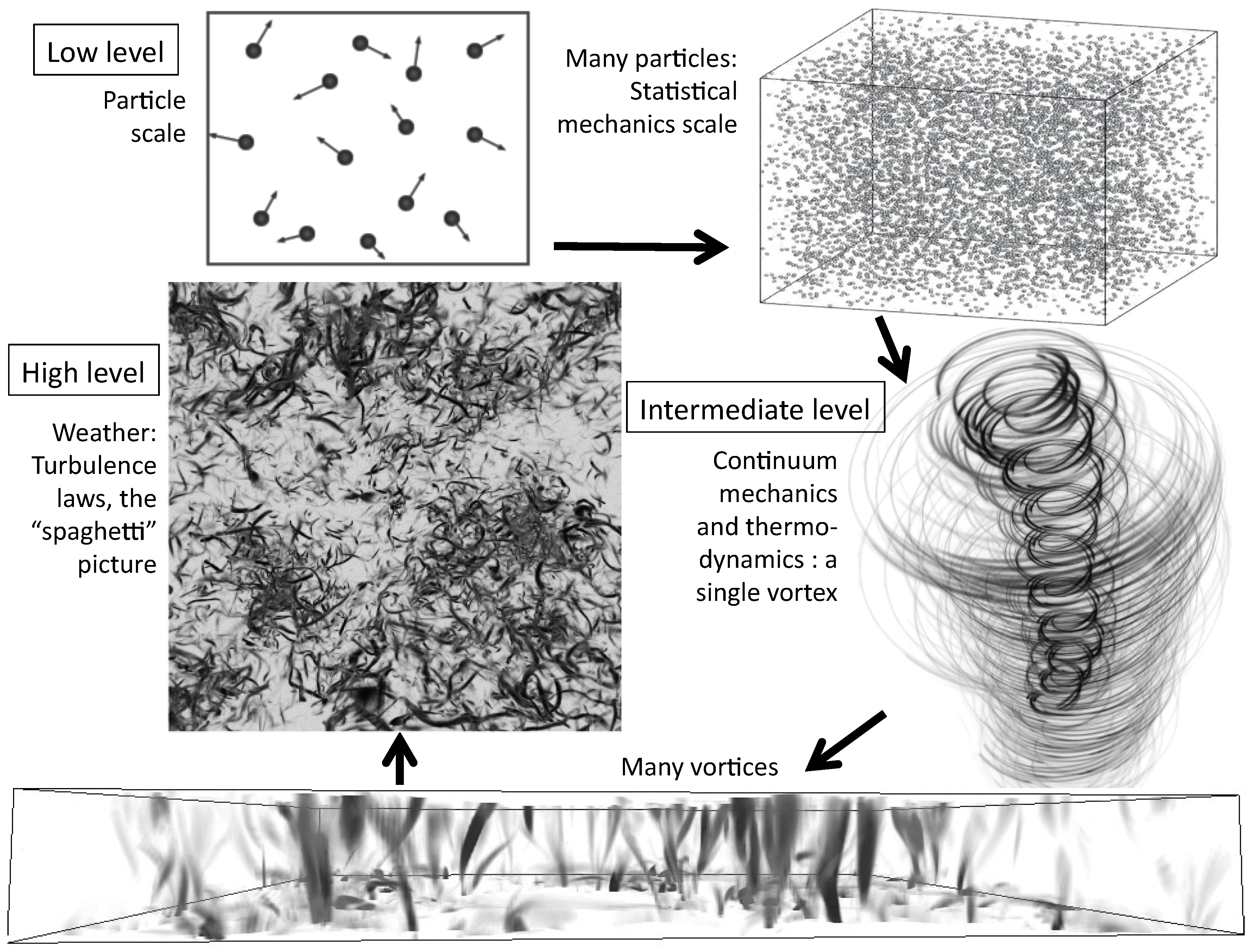
In contrast, the stochastic turbulent strand that Richardson had helped inaugurate was mostly analytical, being initially based on the scaling symmetries of the governing equations (see Appendix C). Harkening back to Maxwell [37] and Gibbs [38], the turbulence approach was motivated by classical statistical physics, it was precisely based on the overarching idea that in systems with huge numbers of degrees of freedom, that most of the details are irrelevant. For example, rather than using (classical or quantum) particle mechanics to chase the details by modelling the positions and velocities of all the molecules in a macroscopic body, one instead attempts to discover higher level laws (statistical mechanics, continuum mechanics, thermodynamics) governing their collective behaviour.
For macroscopic systems, statistical mechanics is superior to particle dynamics not so much because it would save computer time, but because it singles out the relevant aspects of the collective behaviour. From the point of view of modern physics, particle mechanics, statistical mechanics and then continuum mechanics (with thermodynamics) are simply three different levels of modelling and understanding (see Figure 1). However, the hierarchy does not stop there: the turbulent laws that emerge in high Reynolds number flows operate at a still higher level (turbulence). The laws at different levels are mutually compatible, so that for a given application, scientists choose the most convenient level. For example, conventional weather and climate models use continuum and thermodynamics rather than statistical physics. The fact that these continuum theories do not even acknowledge the existence of atoms is a strength, not a weakness. Just as the position and velocities of the constituent particles in continuum mechanics are irrelevant so too are the timing and location of weather events in climate projections. The status of the GCM and turbulence based (stochastic) models discussed below is analogous: they may both be valid models, one chooses one or the other (or may use both together) depending on the problem at hand, depending on convenience. There is no contradiction between them.
Starting in the mid 1970s and early 1980s, the turbulent approach underwent its own revolution: nonlinear physics and geophysics especially deterministic chaos [39,40,41] and fractals [42,43]. From the point of view of atmospheric dynamics, there were two key advances. First, the realization that the scaling symmetry, is a powerful simplifying feature of atmospheric dynamics provided that it is generalized to deal with atmospheric anisotropies especially (but not only) those arising from gravity (differential stratification), and the Coriolis force (differential rotation).
The precise formalism for handling such generalized scaling symmetries is Generalized Scale Invariance [30,44,45], GSI). GSI can be regarded as an appropriate way to transfer into stratified (and possibly rotating) turbulence the classical turbulence insights and theories regarding isotropic, unstratified, nonrotating turbulence. See Appendix B for a more in-depth discussion and Appendix C for the connection with the governing equations.
Richardson’s cascade idea led to the second relevant discovery: that cascades generally lead to multifractals and to the identification of these multifractal processes as the generic scaling processes [30,31,46]. Thanks to multifractal cascades, we can now account for the atmosphere’s enormous intermittency (especially in the weather regime) including the fact that most of its energy and other fluxes are concentrated in violent, extremely sparse (fractal) regions (for reviews, see [5,47,48,49,50,51]). Fortunately, in the macroweather regime, the strong temporal weather regime intermittency is largely averaged out resulting in much lower temporal intermittency. As a consequence, as a first approximation the mean and standard deviation are adequate so that quasi Gaussian modelling may be used [52] (although more extreme random forcing—internal variability—is possible and are probably needed to capture the extremes, see Appendix A).
2.2. The Scaling Revolution
2.2.1. Spatial Scaling Is the Primary Symmetry—Not Isotropy
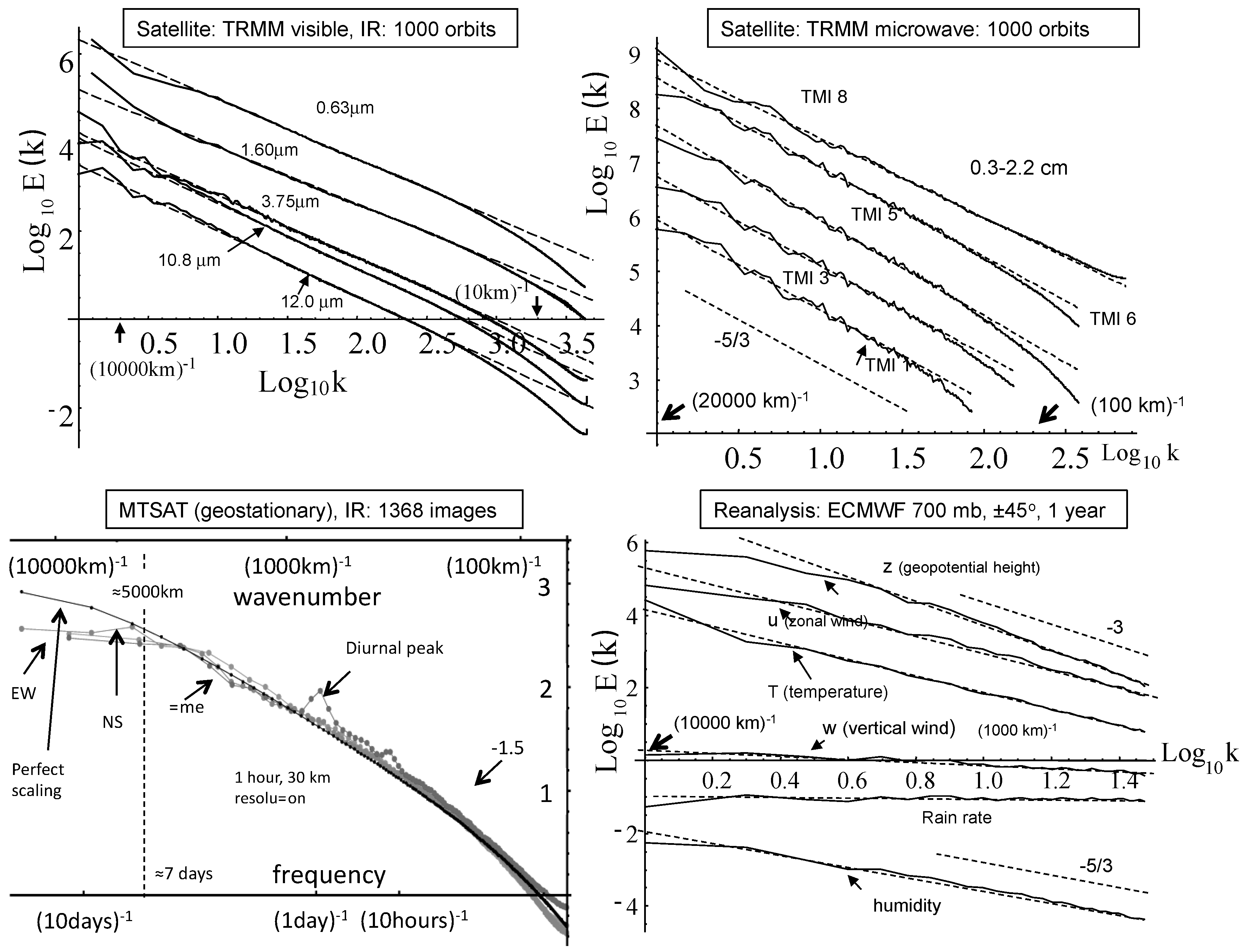
While Richardson’s numerical strand of atmospheric science was vindicated in the 1970s, surprisingly, his wide range scaling, turbulence (stochastic) strand (including the Richardson 4/3 law of turbulent diffusion), was only vindicated much later, thanks to the widespread availability (and subsequent analysis) of global scale data sets both on Earth (Figure 2) and on our twin, Mars. Analysis after analysis has shown the spatial scaling of atmospheric fields. Furthermore, important were the findings that the boundary conditions (including the ocean and topography [53]) are accurately spatially scaling over huge ranges of scales [31,54,55,56,57,58,59,60,61,62]. These empirical scaling studies included direct study of turbulent cascades (in the horizontal [60,63], in the vertical [64], in time, [65], in space-time [66], Figure 2). Using trace moment analysis techniques [31], they not only determined the hierarchy of (multi) scaling exponents but also directly estimated the outer spatial scales of the cascade processes finding that these are of the order of planetary scales (typically 5000–15,000 km). A variety of scaling analysis methods including trace moments, spectra, detrended fluctuation analysis and (generalized) structure functions were applied in situ measurements, radar reflectivities, visible, thermal IR, passive microwave satellite radiances, temperature, wind, pressure heights, humidity, precipitation, potential temperature, aerosol backscatter, cloud densities and in reanalyses and outputs of numerical weather models (see, e.g., Figure 2 and for reviews, refs. [5,50,67]).
The relevant scaling exponents were systematic determined and in several cases, compared to Mars [68]; our sister planet was to found to have quantitatively very similar cascades, spectra and exponents. This similitude is not as surprising as it might at first sight appear: cascades and scaling are fundamental properties of strongly nonlinear turbulent flows. Although it has taken decades to establish, spatial scaling turns out to be a basic property of the governing equations (and hence of GCM outputs).
Scaling is a symmetry that statistically relates small and large scales—or in time, fast and slow processes (Appendix B). Without gravity, isotropic scaling is a fundamental property of the governing equations (Appendix C) that classically has exploited in numerous “similarity” laws (e.g., ref. [69] and it is the basis of theories of isotropic turbulence, Appendix B). The trouble is that gravity breaks isotropy so that the atmosphere is strongly stratified.
Which symmetry is primary: scaling or isotropy? To Richardson—writing before the development of sophisticated isotropic theories—it seemed obvious that it was scaling and he argued that it held from thousands of kilometers down to dissipation scales. However, for complex reasons recounted in Appendix B, following Charney’s theory of geostrophic turbulence, the idea of isotropy primary has been consecrated in models combining small scale isotropic turbulence in three dimensions with large scale isotropic (quasi-geostrophic) turbulence in two dimensions, so that the alternative scaling primary GSI [30,44] alternative (with fractional vorticity equations replacing quasi-geostrophy [70]) has been widely ignored. Fortunately, the GCMs inherit the wide range scaling of the governing equations (Appendix C) so that they can be realistic and the persistence of the outdated 2D/3D isotropic paradigm has no practical consequences for GCM modelling. However, it has unfortunately prevented both an understanding and exploitation of the scaling alternatives (Appendix B).
2.2.2. Scaling in Time: Using Scaling to Define Different Atmospheric Regimes
In physics, symmetries have come to play a fundamental role because the assumption that a symmetry is respected is the simplest one possible and—thanks to Noether’s theorem [71]—they are generally equivalent to conservation laws. For example, energy conservation follows if a system’s Langrangian is invariant to translations in time, and scaling exponents (and more generally group generators) are invariant (conserved) under changes in scale (we have mentioned the conserved exponent H for the mean, see Appendix B.1 more information including for higher order moments). The initial assumption is that a symmetry such as conservation of momentum or energy, is respected unless a specific symmetry breaking mechanism can be found (e.g., a source or sink of energy). In the case of the atmosphere, we have just discussed that both the equations, and now massive data analyses, are horizontally scaling over wide ranges, including the important but nontrivial wind case [72]. Since energy conservation is associated with a symmetry and the scaling symmetry is associated with a conversation principle, in the following for brevity, I will sometimes refer collectively to them simply as “symmetries”.
The spatial scaling of atmospheric statistics leads (especially the key wind field) to the expectation that scaling operates over potentially wide ranges in time. It is therefore natural to use temporal scaling to define the various atmospheric dynamical regimes. Although this idea is hardly new, its application to the atmosphere was obscured by the widespread but inconsistent use of spectral analysis combined with scalebound theoretical frameworks, e.g., the 2D/3D paradigm. (More generally, “scalebound”, Mandelbrot [73] refers to the view that as we zoom into structures that we require a hierarchy of different mechanisms, processes, to explain them and to model them. It is an a priori rejection of the possibility of scaling).
It was only recently realized that the (still) iconic atmospheric temperature spectrum proposed by Mitchell [74] was in error by a quadrillion or so [75]. Writing at the dawn of the climate and paleo-climate data revolution, Mitchell speculated that from hours to the age of the planet, that the temperature variability consisted of an uninteresting (mostly) white noise “background” interspersed with interesting periodic and quasi-periodic processes. Today, in spite of the existence of copious quantities of instrumental and paleodata, Mitchell’s admittedly “educated guess” spectrum is not only still regularly cited but also approvingly reproduced with embellishments (e.g., the review [76]). As discussed in ref. [5], the source of this astronomical error was not with spectral analysis per se but rather with their non-intuitive dimensional units and with the theoretically convenient scalebound mind-set that dominated their interpretation.
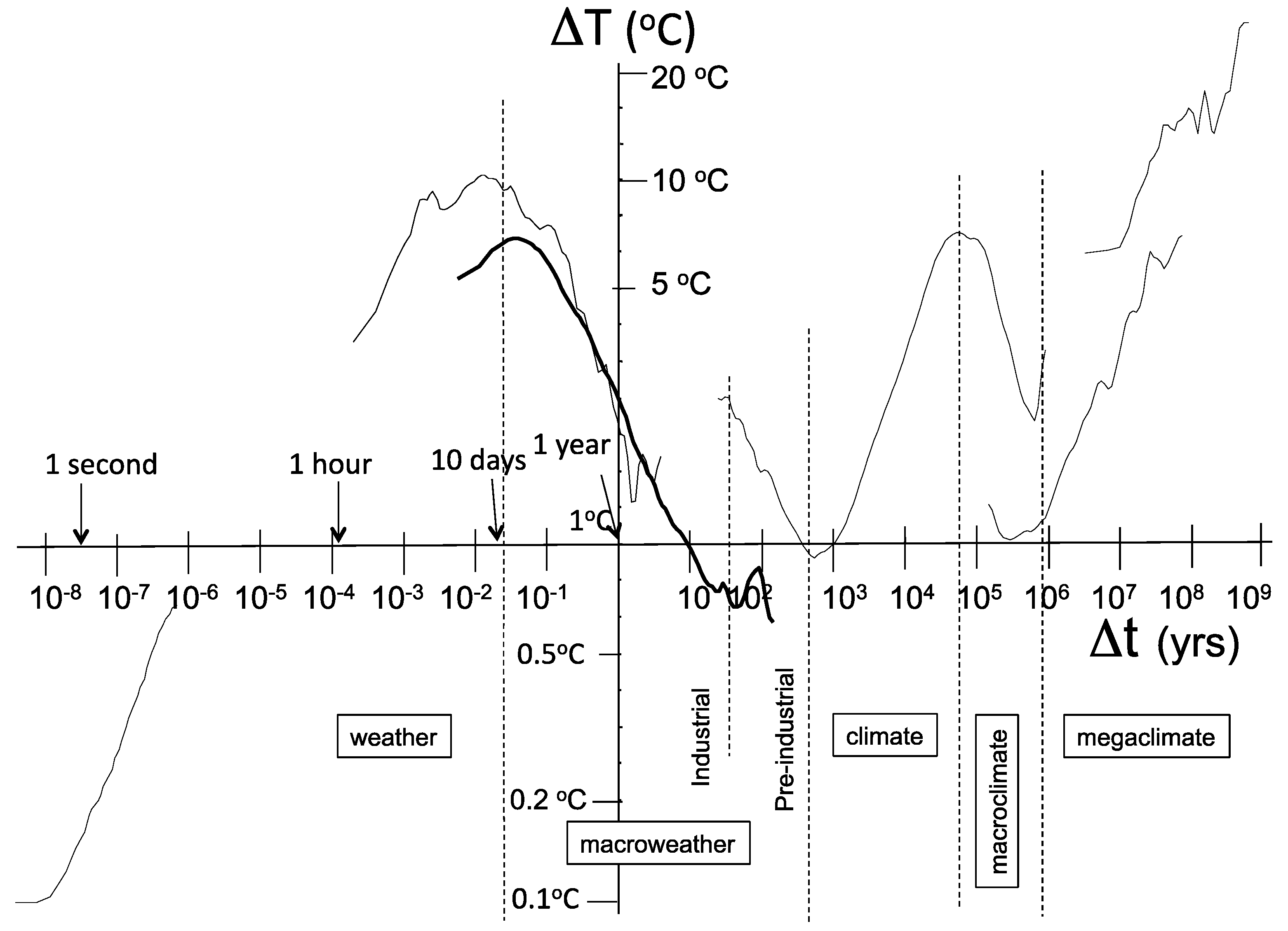
Clarification of the “big picture” atmospheric variability was facilitated thanks to “fluctuation analysis” [77] based on Haar wavelets [78], Figure 3. Over a time interval Δt, the Haar fluctuation in the temperature ΔT(Δt) is simply the difference between the average over the first and second halves of the interval. In Figure 3, we show the root mean square Haar fluctuation using instrumental and paleo-data. The figure clearly shows the existence of four or possibly five dynamical regimes spanning the range from milliseconds to hundreds of millions of years. One notices in particular the alternation of regimes with growing, “wandering” type fluctuations (positive logarithmic slopes, , H > 0) and those with “cancelling” apparently converging negative slopes (H < 0).
Of particular importance is the transition at around ten days that corresponds to the typical lifetime of planetary scale structures. This drastic transition in the statistical properties can be calculated from first principles by assuming that the atmosphere is effectively a heat engine that converts incident solar energy into mechanical (wind) energy. It’s efficiency is ≈ 4%, implying an average power per mass ε ≈ 10−3 W/kg; the same theory explains the analogous fundamental transition on Mars at ≈2 sols with ε ≈ 40 × 10−3 W/kg [79]. Based on these analyses, it was argued that on the Earth—at least up to Milankovic scales (≈105 years)—that there are three fundamental regimes—not two—and that the intermediate regime should be termed “macroweather” with the term “climate” reserved for the long-time positive slope (H > 0) regime in Figure 3 with fluctuations increasing with time scale (see ref. [80]).
On theoretical and empirical grounds, the lifetime of planetary scale structures is itself (nearly) equal to the deterministic predictability limit of these largest structures with smaller structures having shorter lifetimes and limits. Even if we start with a deterministic weather scale model, due to this sensitive dependence on initial conditions (the “butterfly effect”), beyond ten days or so, the model will be effectively stochastic. A complication is that the ocean is also a turbulent system but with ε ≈ 10−8 W/kg (about 10−5 times smaller than the atmosphere), and hence with transition time about 40 times longer so that the corresponding “ocean weather” to “ocean macroweather” transition is ≈1 year [50]. This somewhat longer transition scale turns out to be quite variable from place to place ranging from a month or so to a year over the El Nino region [20]. It implies that there is still some deterministic prediction skill for ocean systems (e.g., gyres) beyond the atmospheric transition scale; for monthly resolution macroweather forecasts, this turns out to be a manageable complication [20].
3. The Fractional Energy Balance Equation (FEBE): A First Generation Macroweather, Climate Model
3.1. FEBE’s Physical Basis
The weather—macroweather regime is defined by the lifetime of planetary scale structures which turns out to be essentially equal to their deterministic predictability limit. At macroweather scales, weather scale dynamics based on classical fluid dynamics therefore effectively becomes stochastic with statistics determined by the collective behaviour of huge numbers of short lifetime, small scale “details” [40]. Constructing a model directly at biweekly or monthly scale macroweather scales thus naturally retains relevant parameters while jettisoning many irrelevant details.
From the modelling point of view, the augmentation of the model’s integration time step from subhourly to monthly is already hugely advantageous, but since time and space are linked, computational savings do not stop there. In the weather regime, the lifetimes of structures (τ) increases with their size (l) as ; this leads to the rule of thumb that every halving in spatial resolution requires at least a ten-fold increase in computations [2]. In macroweather models, not only is the space-time relationship quite different, but most importantly, only statistical relationships are relevant. If the goal is to accurately account for as many details as possible, then unsatisfactory subgrid parametrizations are needed (Appendix A). In contrast, in stochastic macroweather models, the aim is instead to understand/model/capture the statistical scaling laws. A climate projection at a given spatial scale, can be made without modelling the finer scales since their collective statistical effects are already included in the model’s stochastic scaling laws. Below, we present climate projections performed on laptops, not supercomputers.
However, what physical principles should macroweather models embody? Above, I argued that they should respect the scaling symmetry, and indeed scaling climate models have been proposed for some time [23,81,82,83]. However, on its own, the scaling symmetry is a rather loose constraint, and without care it can lead to the “runaway Green’s function effect” [23,84]. It is therefore advantageous to combine it with other symmetries, the obvious one being energy conservation (i.e., time-origin invariance). Indeed, starting with refs. [16,17], in the form of energy balance models (EBMs) energy conservation has a proven track record (see the recent extensive review [85], and update [86]).
It turns out that the symmetries of scaling and energy conservation come together quite naturally. To illustrate this, for simplicity consider the EBM for the globally averaged temperature (the “zero dimensional” special case of regional EBM models):
where T(t) is the temperature anomaly, τ is the relaxation time, s the Equilibrium Climate Sensitivity (ECS) and F(t) the forcing that includes both external (deterministic Fext) and internal (Fint, e.g., white noise) contributions. Note in the above equations all the quantities refer to global scale so that for example, in Equation (1), T(t) is the global mean macroweather temperature anomaly, traditionally taken at one month resolution with respect to one month averages over a 30 year reference period (the “baseline”). However, the linearity of the energy balance equations means that there is much flexibility in the definition (for example they can be defined with or without seasonality, seasonal or annual anomalies, etc. Interestingly ref. [87] has applied the anomaly idea so as to derive an anomaly model from the governing equations.
However, the classical Budyko–Sellers derivation of the EBE was for the distribution of temperature on the Earth’s surface (not just the global average), this was averaged so as to obtain a 1-D latitudinally varying model. To understand this, we now discuss a full regional model with regionally varying anomalies and parameters. Their derivation involved the approximation that any imbalance between the incoming short wave and outgoing long wave radiative fluxes is directed horizontally towards the poles. However, in reality, some of the imbalance increases the local (regional) temperature leading to increased outgoing long wave radiation, and some of it is converted into sensible heat that is conducted into the subsurface and stored (coming out possibly much later). To take this radiative-conductive boundary condition into account, we must introduce the third (vertical) spatial dimension (with coordinate denoted by z). At the surface (z = 0), the sensible heat equals (K is the is the thermal conductivity) whereas the radiative flux is T/s where s is the local climate sensitivity. Overall, the precise radiative-conductive boundary condition is: [88,89].
Using the conductive-radiative boundary condition we can now consider the full space-time classical heat equation (Fourier’s and Fick’s laws), so that we obtain the regional Half-order Energy Balance Equation (HEBE):
where ζ is the horizontal divergence operator, are the two dimensional (surface) gradient and divergence operators, nondimensionalized by the Earth radius, (i.e., the spherical angular parts of the operators), μ is the cosine of the co-latitude, ϕ is the longitude, and D is a heat diffusion coefficient. As indicated, the parameters τ, s, D are functions of latitude and longitude; T, F are also functions of time. For a different application of half-order operators in soil heating see ref. [90].
The longitudinally averaged case considered by Budyko and Sellers has only latitudinal dependence, , their model is then the special case of Equation (3) with χ = 1 instead of χ = ½ (assuming s is constant). Interestingly, the Fractional Energy Balance Equation (FEBE) that uses the radiative-conductive surface boundary condition but with the fractional heat equation (instead of the classical heat equation), is actually:
We see that the HEBE (Equation (4) with χ = 1/2), is the special case of the FEBE with h = 1/2 (compare Equation (4) with h = 1/2, with Equation (3) with χ = 1/2), however, the Budyko–Sellers model is not a special case of the FEBE (Equation (3) with χ = 1). This is a consequence of the fact that the Budyko–Sellers model involves an important approximation and does not satisfy the radiative-conductive boundary conditions. In both Equations (3) and (4), the term in parentheses is a fractional space-time operator that needs to be carefully interpreted [88,89]. Just as fractional derivatives in time imply long range (power-law) temporal dependencies, divergences in horizontal heat fluxes (ζ) analogously imply long range spatial dependencies. The full (regional) FEBE (Equation (4)) is a space-time model of the Earth’s temperature that accounts for both stochastic internal variability as well as the deterministic response to external forcings.
Finally, the globally averaged (zero-dimensional) FEBE is obtained from Equation (4) with ζ = 0:
The classical heat equation yields the HEBE with h = ½ not the “box” model or “zero-dimensional” version of the Budyko–Sellers model that has h = 1. Alternatively, Equation (5) with h ≠ ½ may be derived directly on phenomenological grounds [91]. The physically relevant range is probably 0 < h ≤ 1 since over the range 1 < h ≤ 2, there are oscillations that are probably not realistic. Technically, the h-order derivative is a Weyl derivative, in the frequency domain it is a power law filter: where F.T. indicates Fourier Transform. In real space, fractional derivatives are power law convolutions so that the half-order derivative is an expression of the slow (power law) transfer of heat into and out of the earth’s subsurface (land or ocean). Mathematically, it is an expression of the Mori-Zwanzig or empirical model reduction formalisms that are usually assumed to involve integer ordered derivatives (e.g., ref. [76]). These classical derivatives are exceptional in that they have exponential rather than power law Green’s functions. The HEBE is apparently the first power law instance in the literature.
The globally averaged EBE, HEBE and FEBE (Equation (5) with h = 1, h = ½, 0 < h < 1 respectively) are relaxation equations. When forced with deterministic (e.g., anthropogenic) and no random forcing (i.e., in Equation (2), Fint = 0), they govern the return of the temperature to its equilibrium value following a perturbation. For example, if F(t) represents an instantaneous doubling of CO2 (step function)—then with fractional h, the approach of the temperature to its new equilibrium is .
Since the Fourier Transform of the half order derivative in Equation (5) is , if τ, s are independent of time, then we may easily solve the above: where the tilde indicates Fourier transform. This is particularly convenient if we wish to understand the behaviour of the system when forcing by random internal variability. For example, if F is a white noise forcing of amplitude σ, then the spectrum is:
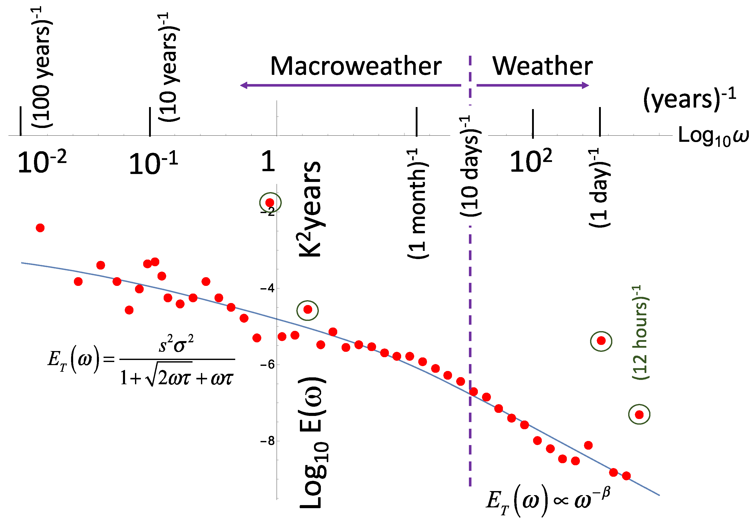
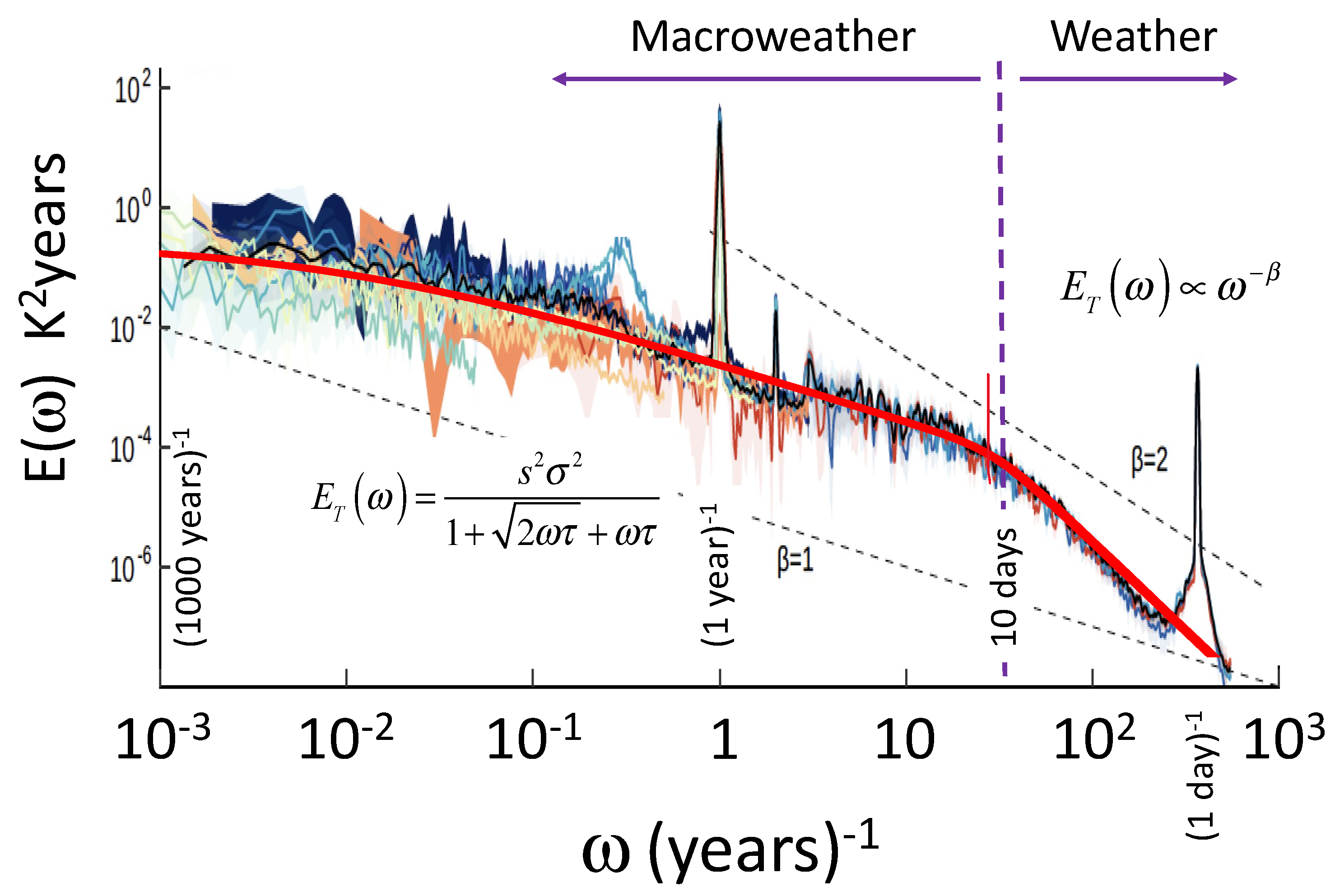
For the HEBE (h = 1/2 in Equation (6)), we obtain: ; Figure 4 and Figure 5 show that at times longer than the typical weather-macroweather transition scale (about ten days for the globally averaged temperature, there are regional variations) that the HEBE is indeed well respected. Although the figures show that the HEBE is already an excellent approximation h may not be exactly equal to 1/2 and it can be empirically estimated in several ways. For example, using the response to (stochastic) internal variability, ref. [18] found h = 0.42 ± 0.05, and using the response to (deterministic) forcing, ref. [6] found h = 0.38 ± 0.03 (see below).
If the internal forcing Fint is a Gaussian white noise (see, e.g., ref. [52]), then the FEBE response is a “fractional Relaxation noise” [92] (fRn) that at high frequencies (Δt ≪ τ) is nearly a (more familiar) fractional Gaussian noise [93] (fGn) that has fluctuations with scaling exponent (logarithmic slope) H = h − ½ < 0. While the white noise internal variability forcing has typical fluctuations decreasing as , the external anthropogenic forcings ΔFext instead increases with time scale therefore eventually becoming dominant. (Of course—as mentioned earlier—the weather scale processes responsible for the internal forcing are ultimately multifractal with strong extremes, Gaussian internal variability is only the simplest model and in the future this assumption can be relaxed).
At this point we might mention that the scaling symmetry only applies to the fractional term that represents the imbalance between the incoming short wave radiative flux F and the outgoing long wave flux T/s. In Equations (1) and (5) (the global averaged model) or in the regional model (Equation (4)), neglecting the horizontal divergence term ζ, it corresponds physically to energy storage processes that are therefore scaling. From the spectrum (Equation (6)) we can see that the overall behaviour of the temperature statistics has both a power law approach to equilibrium (the low ω limit) as well as a power law high ω limit).
3.2. Using the FEBE to Project Temperatures to 2100
3.2.1. FEBE Parameters
Figure 3 helps us to understand how the FEBE can be used for projecting the temperatures at multi-decadal time scales through to the year 2100. First, recall that the shortest time scale that the FEBE may hope to model is in the macroweather regime (with Δt >≈ 10 days) where fluctuations from the internal variability decrease as time scales increase. However, the external anthropogenic forcings ΔFext instead increases with time scale therefore eventually becoming dominant. In Figure 3, the bold curve showing the minimum is from data at 75° N, at 2° × 2° spatial resolution and is from data taken over the last 140 years. The minimum occurs at Δt ≈ 50 years where the root mean square fluctuation of the 50 year temperature anomaly is ≈ 0.7C (i.e., ±0.35 C). This is roughly equal to the average anthropogenic change in temperature at this latitude averaged over the (nearly) three 50 year intervals since 1880. Note that the earliest interval had a smaller change than the recent one and the curve shows the average over the three intervals. If we consider instead the globally averaged temperature (not shown), and consider the most recent decades (with fastest warming), the cross-over from internally to externally dominated forcing occurs at Δt ≈ 10–15 years at 0.1 C. This means that while the typical decadal warming is about 0.1 C, the amplitude the typical decadally averaged internal variability is ≈±0.05 C.
This cross-over from an H < 0 to H > 0 regime defines the macroweather—climate transition (in our current epoch). It shows that for climate projections until 2100, the FEBE can be forced using the anthropogenic forcings. In the pre-industrial period, there is still debate as to the length of macroweather—climate transition scale. It is certainly much longer—possibly multi-millenial—and is still not well understood [94,95,96]. However—if only due to the existence of ice ages representing changes of several degrees at ≈105 year time scales—there is no question that fluctuations must reverse their decline with scale—and start to increase, as shown by the EPICA ice core in Figure 3.
The basic FEBE (Equation (6)) is a linear equation so that the deterministic responses to anthropogenic forcings can be considered independently of the (superposed) stochastic responses to internal forcing. From the globally averaged Equation (6), we see that the relaxation time τ can be used to nondimensionalize time (i.e., t → t/τ): τ determines the (slow, power law) time scale of the relaxation to equilibrium. As usual, the qualitative behaviour of the differential equation is determined by its highest order derivative h, here it determines the stochastic and deterministic response exponents. Finally, the ECS s, quantifies the sensitivity of the temperature to a given power per area of forcing.
In order to exploit the FEBE for projections, Bayesian inference was used based on historical records of past global temperatures. Reconstructed forcings at monthly resolution is convenient, here I used those from the CMIP5 and CMIP6 simulations. The Bayesian methodology was first developed in ref. [23] for the somewhat different Scaling Climate Response Function (SCRF) model, and then applied to the FEBE in refs. [6] (see also ref. [21] that also has regional FEBE projections). Bayesian inference transforms available initial knowledge into prior probability distributions. These are then confronted with data to produce a posteriori probabilities using Bayes theorem. The last step requires a hypothesis about the a posteriori likelihoods. Whereas traditionally these are not well known—and are thus usually ad hoc—an elegant feature of the FEBE is that they are given by the model itself. This is because the FEBE determines both the deterministic and stochastic responses, and the latter (the response to the internal variability white noise forcing) determines the likelihoods.
Before presenting parameter estimates and projections [6], a word about the historical forcings is needed. The main issue is the role of aerosols that are particularly uncertain so that are not so well reconstructed. This problem was dealt with by introducing a linear parameter α that determined the overall aerosol strength by renormalizing the (somewhat different) AR5 and AR6 aerosol reconstructions (the two gave quite similar results, only the former is shown below). A final forcing issue is the intermittency or “spikiness” of the volcanic forcing. In order to fit volcanic forcing into the linear response framework, a nonlinear transformation is needed, determined by an empirical exponent ν. The global temperature response data are also somewhat uncertain. As a consequence, five different monthly resolution data sets since 1880 were used with each given an equal a priori probability [6].
With this data, the median FEBE parameters were estimated as h = 0.38, [0.33–0.44], τ = 4.7, [2.4–7.0] years, s = 2.0, [1.6–2.4] C/CO2 doubling with the square brackets indicating the 90% “credible intervals”. (In Bayesian statistics, the credible interval is the interval within which an unobserved parameter value falls with a particular probability. It is the Bayesian analogue of a “confidence interval”). These FEBE parameters may be compared with the classical EBE value h = 1 (integer order theory from Equation (2)), τ = 4, [2–6] years (from General Circulation Models, GCMs [97]; unpublished analyses using the HEBE show that there is a wide range of regional relaxation times varying from less than a month (many land areas) up to millenia for some tropical ocean areas).
For the important equilibrium climate sensitivity, s, see Table 1. In the table, we have included the parameters of the SCRF model that was the pre-cursor of the FEBE. In the table we see that the 90% FEBE confidence interval lies completely within the AR5 expert range and largely overlaps the AR6 MME range. Note that strictly speaking, MME uncertainties are classical “confidence intervals” whereas the Bayesian uncertainties are “credible intervals” (CI). In the former case, they arise because of “structural uncertainty”, i.e., the differences in how the various members of the MME were constructed. In the latter case, they are parametric uncertainties (uncertainties in the model parameters) largely due to uncertainties in the past forcing reconstructions and historical temperature series.
3.2.2. FEBE Hindprojections
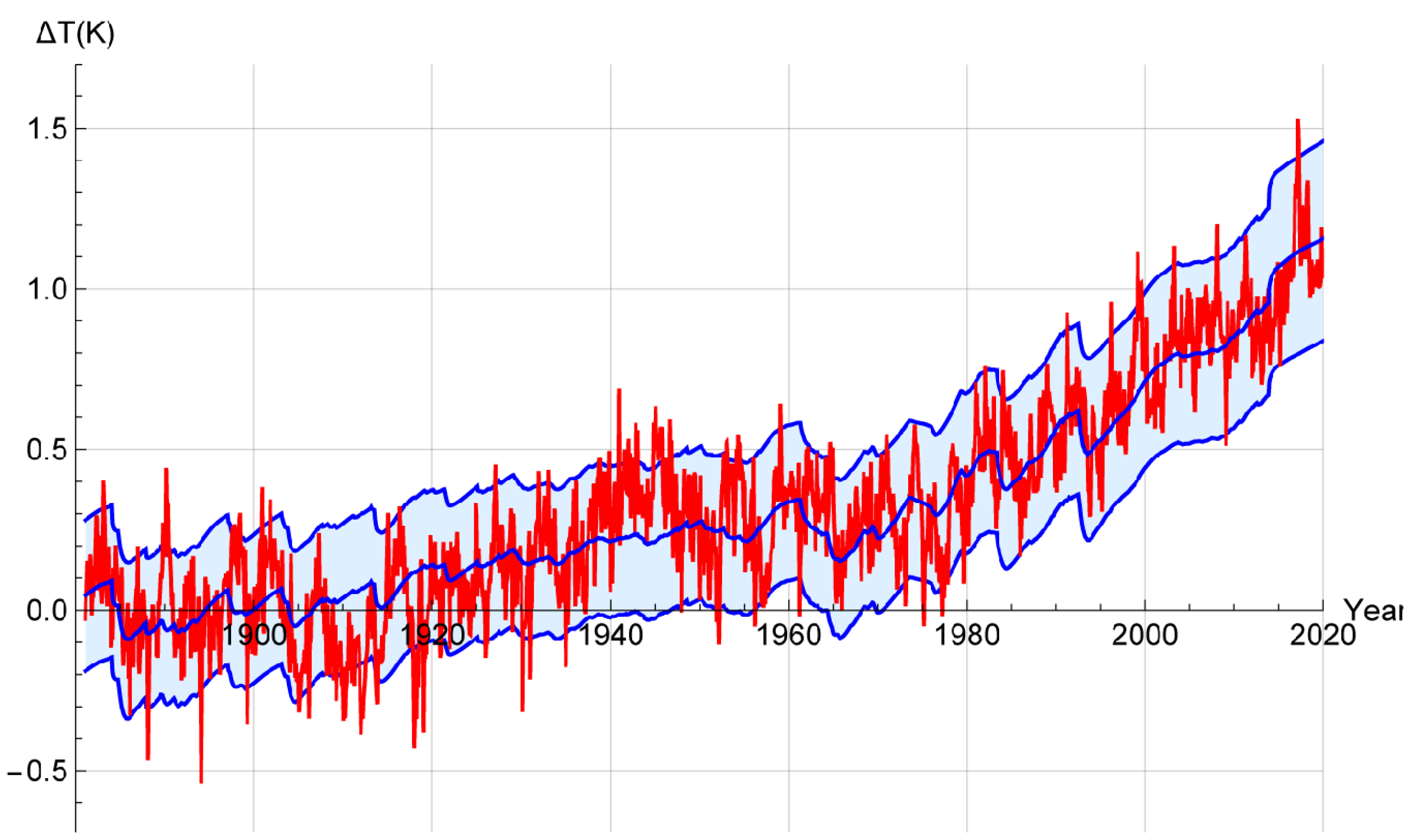
Projections throughout the 21st century can now be made using the model, the estimated parameters, the historical forcing and the (prescribed) future forcing scenarios. Before showing the future projections, it is worth verifying the model by comparing the model hindprojections with the historical temperature data. This can be done in two ways. First, one can test the FEBE “reliability” (Figure 6). The reliability is a technical term that quantifies the difference between the forecast and actual probability distributions. For example, consider a set of long range weather predictions derived from ensemble forecasts. In some realizations, it is predicted that the chance of above average seasonal-mean temperature for the coming season is 60%. If the probabilistic forecast system is reliable, then one can expect that in 60% of these predictions, the actual seasonal-mean temperature will be above average [101,102]. Figure 6, verifies that the reliability of the FEBE is as expected: it shows that the temperature observations fall closely within the 90% credible interval (CI) of the FEBE historical reconstruction (i.e., the ensemble average of the response with both internal and external forcing). More precisely, at Figure 6′s monthly resolution, the historical mean temperature (red) is within the 90% CI of the FEBE-forced response 89.9% of the months using the RCP scenario with internal variability added. The accuracy of this uncertainty verifies both the underlying model and Bayesian parameter estimation method.
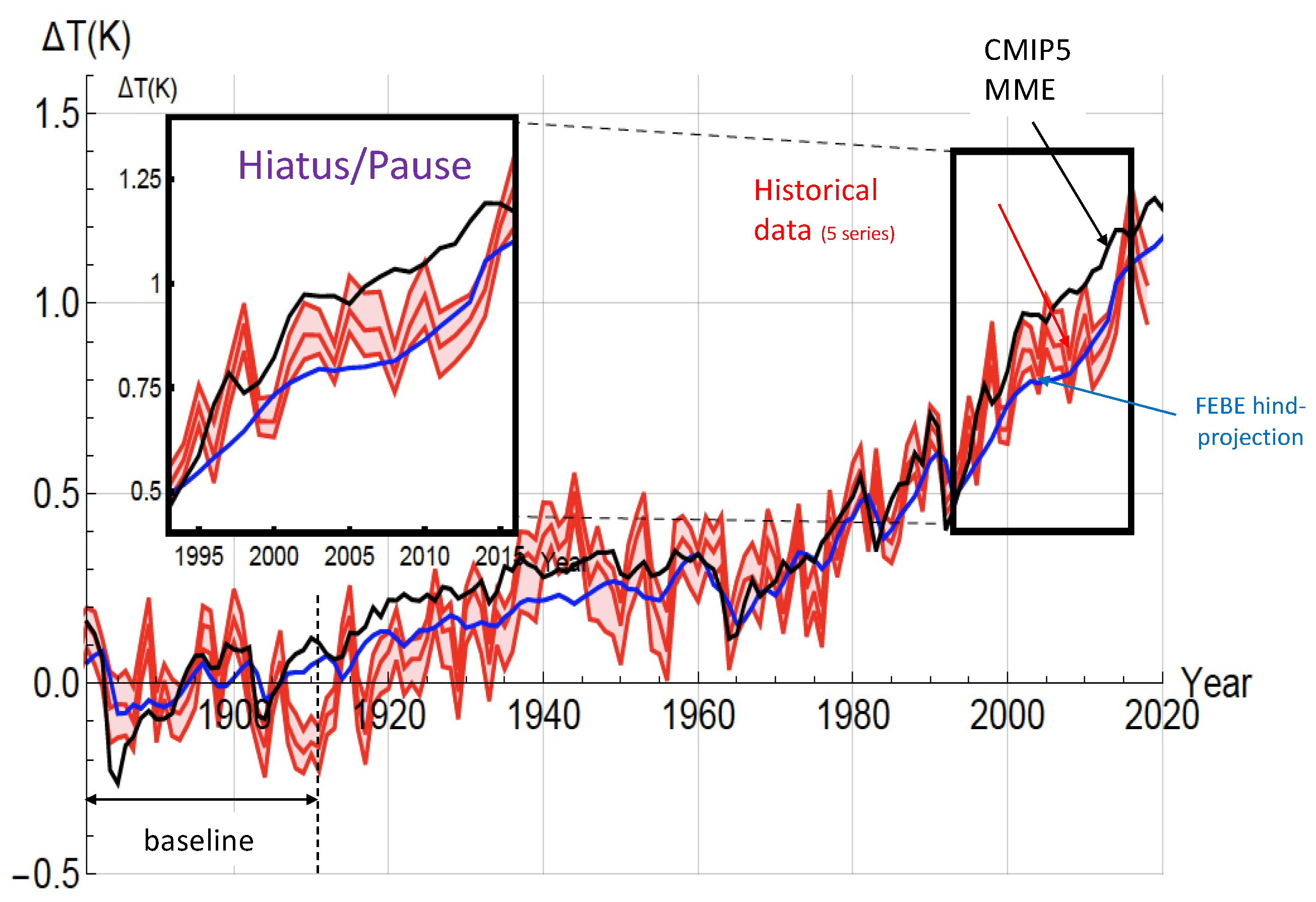
The reliability validation in Figure 6 included the internal variability; in Figure 7 we show an estimate of the ensemble averaged hindprojections, i.e., with the internal variability completely averaged out. This is not a reliability check, so we do not expect the ensemble averaged FEBE to be in the data range 90% of the time. Rather, the percentage of the time that the ensemble averaged FEBE is in the data range is a measure of hindprojection—data agreement about the deterministic forced response part. It is therefore appropriate to compare this with the MME. In Figure 7, we compare the 90% CI of the historical temperature observations with the median forced response of both the FEBE using the CMIP 5 Representative Carbon Pathway 4.5, the number “4.5” refers to the increased scenario forcing in the year 2100 in W/m2 (see ref. [6] for comparison with CMIP6 models and further discussion).
In the inset of Figure 7, we show the “slowdown” (“hiatus”) period (1998–2014). Throughout the historical period, the hindprojection of the FEBE and the median of the CMIP5 MME are close (see ref. [6] very similar CMIP6 graphs). Between 1915–1960, the CMIP5 MME is consistently warmer than the FEBE hindprojection and warmer than historical temperature records between 1910 and 1935, although generally by less than 0.05 C. The slowdown in global warming during the first decade of the 21st century [103,104], is tracked closely by the FEBE hindprojection, while the CMIP5 MME median overshoots (by 0.1 to 0.2 C)—a well-studied divergence between GCMs and observations—is shown in Figure 7 (insets). This supports ref. [105], who found that the slowdown could be well predicted by a stochastic fGn model (comparable with the present hindprojection).
3.2.3. FEBE Projections
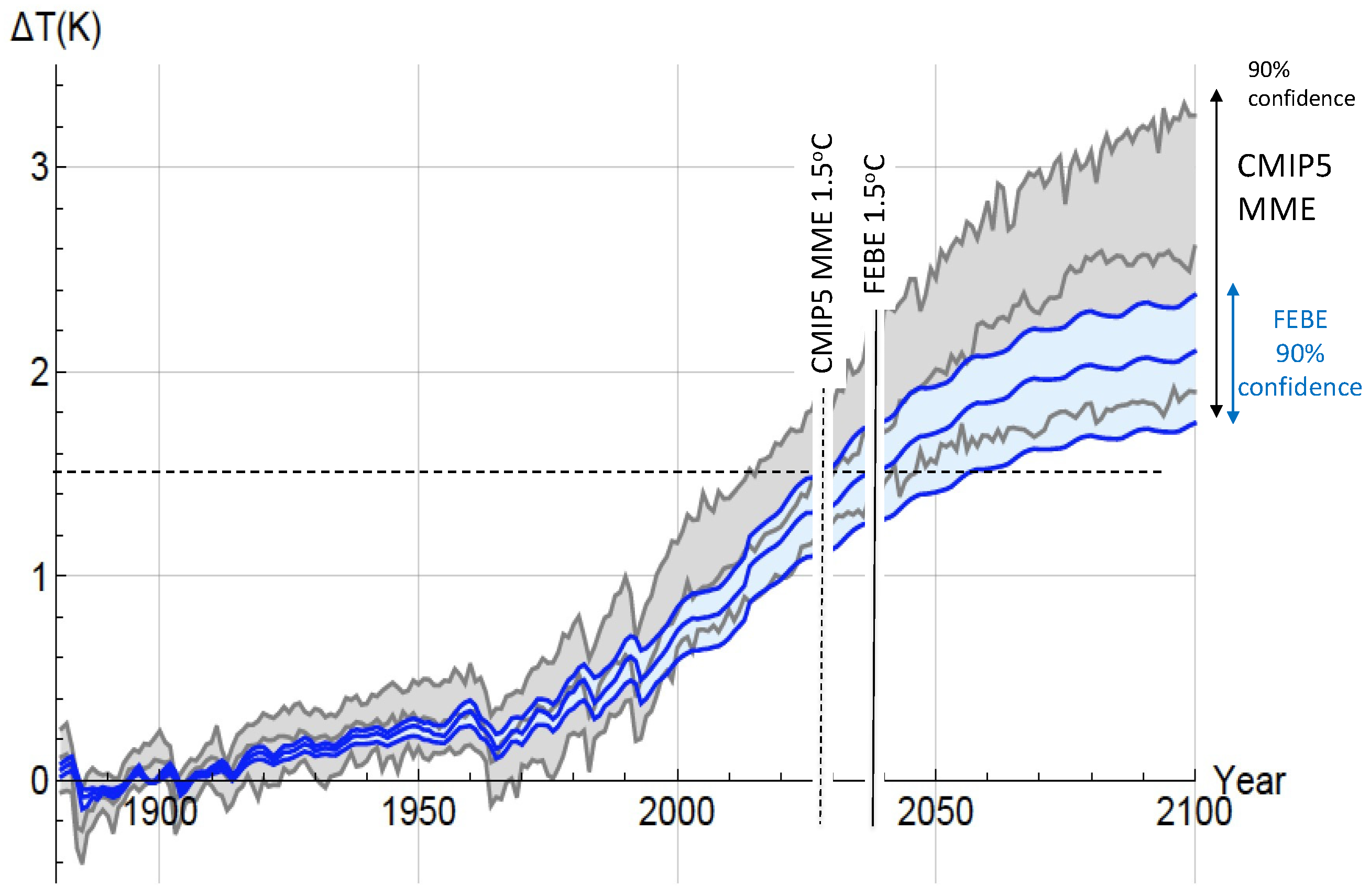
From Figure 6 and Figure 7, we see that the FEBE is reliable (Figure 6) and well reproduces the globally averaged past temperatures (Figure 7). In fact, the Bayesian approach allows us to determine the entire (joint) multi-parameter probability distribution in the 5 dimensional (h, τ, s, α, ν) parameter space. This implicitly includes the correlation information between the parameters (i.e., the fact that estimates of certain parameters—for example h, τ are correlated). Combining this joint parameter probability distribution with the past forcing data and future forcing scenarios, we can make future projections. The simplest way is to use a numerical Monte Carlo method that draws parameters at random from the 5 dimensional (h, τ, s, α, ν) space and then for each set, to use the FEBE to integrate forward to the year 2100.
The result—for the moderate mitigation scenario RCP4.5 is shown in Figure 8 (for other AR5, AR6 scenarios, see [6]). The most important point is the near complete overlap of the 90% confidence limits for the two different models that implies that they are in complete agreement: the FEBE thus validates the MME and the MME validates the FEBE. This is significant since their uncertainties have quite different origins (i.e., parametric versus structural). We also note that due to the smaller s, that the uncertainty spread is about half that of the MME and that the median FEBE projection is a little lower than the MME.
3.3. Using Macroweather Models to Project CMIP: Model Verification and Hybrids with GCMs
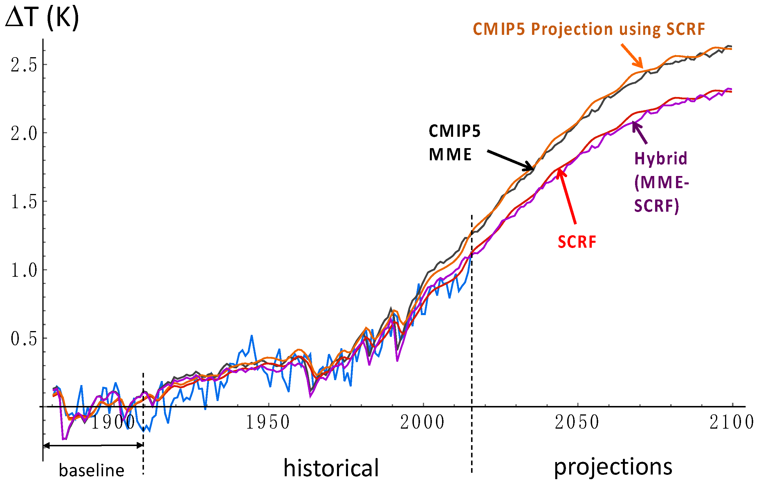
We mentioned that ref. [10] found that in the various AR5 RCP scenarios, that the CMIP5 models (nearly) linearly projected their past (from hindprojection) warming patterns into the future. This linearity suggests that linear stochastic FEBE type macroweather models could be used to project each of the CMIP5 MME members individually. Figure 9 (top curves) shows the result when this is done on each of 32 CMIP5 members [106]. The black curve in the figure is the CMIP5 MME median for the RCP4.5 scenario. Superposed (orange) is the projection of the same CMIP5 models with the same forcings but using the SCRF macroweather model (the close precursor of the FEBE, it has the same parameter set as the FEBE although they have slightly different meanings and values, see Table 1).
For each CMIP5 MME member, the optimum SCRF parameters are estimated from the historical part of the member’s CMIP5 run (its hindprojection), effectively replacing the actual historical temperature data by the model’s reconstruction. Having estimated the SCRF parameters, the SCRF is then used to project the member’s future using the same scenario forcings. The close agreement between the CMIP5 MME median (Figure 9, black, the same as the MME median curve in Figure 8) and the SCRF equivalent (Figure 9, orange) is a validation—at least for globally averaged temperatures—of the stochastic macroweather SCRF. If the SCRF can accurately project the CMIP5 MME using the CMIP5 hindprojection temperature series as inputs (orange), then presumably its projections using real historical data (Figure 9, red) are equally trustworthy.
The successful SCRF projection of the CMIP5 MME raises the possibility of combining the CMIP5 models with the SCRF to make an even more accurate “hybrid” projection (Figure 9, purple). The hybrid projection is the result of taking the SCRF historical data projection with individual CMIP5 outputs as linear co-predictors, weighting the two so as to maximize the standard mean skill score (equivalent to minimizing the error variance) over the historical part of the series (the discrepancy in response with CMIP5 is almost certainly largely due to problems in the observational datasets of that time, notably the lack of accounting for coverage bias, see ch. 3 of the AR6). Whereas the CMIP5 models correct the SCRF biases, the SCRF model corrects the CMIP5 biases. Although suppressed for clarity in Figure 9, the uncertainties of the CMIP5 models are indicated in Figure 8, and the SCRF uncertainties are comparable to the FEBE uncertainties in Figure 8. The hybrid projection has lower uncertainty than either the MME or the SCRF, in future, the method could be applied to the FEBE and to regional projections.
4. Conclusions
There is wide agreement that improvements in multidecadal climate projections are urgently needed to help guide Greenhouse gas mitigation policies and the measures humanity must take in order to adapt to a warming planet. Shortly after the first [107] climate model, the NAS concluded that a doubling of CO2 would lead to 1.5–4.5 C of global warming. Since then, computer power and algorithmic efficiencies have improved by ≈1011, ≈106 respectively. Model resolution has become greater and greater and more and more processes have been included, yet the MME uncertainty has not narrowed. On the contrary, following a disappointing decade, the CMIP6 models in the IPCC’s latest AR6 report in 2021 had an even larger 90% confidence spread: 2–5.5 C/CO2 doubling. As a consequence, the AR6 had to rely more than ever on observation-based constraints and expert judgment to bring the range down to the much narrower range 2.5–4 C/CO2 doubling. In addition, for regional projections, there are serious reasons to doubt the accuracy of the warming patterns [10]. The “uncertainty crisis” is no longer “looming” [5], it is now fully upon us.
The still dominant view—reiterated in a Royal Society briefing [2]—is that “bigger is better” with the overriding goal remaining to produce kilometric scale climate models by the year 2030. However, kilometric structures live typically for 15 min and such models would effectively make centennial scale weather forecasts whose details are known in advance to be wrong. The model outputs would be averaged over a factor of time scales approaching a million, confirming that almost all the expensive details are irrelevant. As shown in Appendix A, even if the goal is to quantify extreme weather-scale events such as extreme daily maximum temperatures, getting a reliable estimate of the mean future climate state is still necessary (it may also be sufficient, see Appendix A).
Indeed, beyond the deterministic predictability limit of about ten days (the atmosphere), the models become stochastic, so that atmospheric scientists should avail themselves of the progress realized in the stochastic strand of atmospheric science to directly build stochastic macroweather models. These include not only the one point statistics that describe the means and extremes, but also the (two point) space-time correlation functions as well as the general (multi-point) joint probabilities, etc. Just as continuum mechanics and thermodynamics jettison the irrelevant molecular scale details, retaining only the relevant macroscopic ones, so too can macroweather models be based on the relevant stochastic laws that account for the collective behaviour of huge numbers of interacting atmospheric structures and processes.
Of course the difficulty is to figure out what is relevant and what is not. Although in this commentary, I do not purport to give any definitive answer, I nevertheless argue that such a model should have the following characteristics: it should be (a) stochastic, (b) grounded in the macroweather regime, (c) use the principle of energy conservation, (d) the principle of scale invariance (scaling, see Appendix B and Appendix C for detailed discussions).
In order to make this plausible we recalled some of the relevant theoretical and empirical developments since the 1970s nonlinear revolution. We argued that an early candidate macroweather model (at least for the surface temperature) is provided by an update of classical Budyko–Sellers type energy balance models. By using the correct radiative conductive boundary conditions, it turns out that these classical equations for heat transport yield half-order fractional derivative equations for the surface temperatures [88], that can easily be generalized to the Fractional order Energy Balance Equation (FEBE, [91]). Since the fractional derivative term corresponds to a power law convolution, the FEBE combines scaling symmetry and energy conservation, and can therefore be tentatively proposed as a suitable candidate model.
With the help of Bayesian inference, the FEBE was recently used to estimate the model parameters (including the Equilibrium Climate Sensitivity) and also to make projections through to the year 2100 (Figure 8). The most important conclusions were that the FEBE and the CMIP model MME were in near complete agreement, yet the FEBE uncertainties were about half those of the MME. When compared to the historical past (since 1880), the FEBE was more reliable (Figure 6) and also in closer agreement with the global mean temperature (Figure 7). Although we mostly discussed the simpler globally averaged model for the temperatures (although see Equation (4)), regional FEBE models have been made (ref. [21]) and in the future, numerous improvements and generalizations are possible. Finally, using the SCRF model (the FEBE precursor stochastic macroweather model), we further showed (Figure 9) that the skill of such stochastic macroweather models can be validated by using it to project the individual CMIP models. If the SCRF or FEBE can accurately project each CMIP5 member using the member’s own past projection, then surely its projections based on real temperature data are equally trustworthy? The success of stochastic macroweather models to project each MME member justifies combining the two in a hybrid scheme that maximizes the overall hindprojection skill. Recent improvements in observational temperature datasets will only enhance the utility of FEBE and other stochastic models that can take full advantage of these advances.
This exemplifies in a practical way the main argument of this commentary: that atmospheric processes can be modelled at different levels reflecting high and low level laws that can be mutually compatible.
We could also mention that the same FEBE model applied to monthly, seasonal and Interannual forecasting produces [18,19,20] state-of-the-art long range forecasts whose skill is provided by their long memories; mathematically rather than being classical initial value problems they are past value problems. In future, various nonlinear extensions—for example for past climate temperature-albedo feedbacks—could allow the model to be applied to past climate modelling including glacial- interglacial transitions. Future developments on such “seamless” stochastic macroweather models could potentially span both macroweather and climate regimes from a month to ice age scales.
Funding
This research is fundamental and received no direct funding.
Data Availability Statement
The only original data analyses are Figure 4 and Figure 5, the other data were only reviewed in this paper, details of their data can be found in the references that were given. Figure 4 used data from the (publically available) NCEP reanalysis as indicated in the caption (https://www.esrl.noaa.gov/psd/thredds/fileServer/Datasets/ncep.\reanalysis/surface_gauss/air.2m.gauss). Figure 5 is an apporoximate fit a curve in the published graph in ref. [94]. The data reference may be found in ref. [94].
Acknowledgments
I thank Raphael Hébert, Roman Procyk, Lenin del Rio Amador and David C. Clark for useful discussions. I also thank anonymous referees for helpful comments and suggestions.
Conflicts of Interest
This is fundamental research. There were no conflict of interest.
Appendix A. The Details and Weather Scale Extremes
The notion that many of the details of a system with huge numbers of degrees of freedom may be irrelevant is the basic idea of statistical mechanics. A familiar example is the central limit theorem that is regularly used to justify the Gaussian distribution of errors. If one takes the sum of a large number of identically distributed independent random variables, then—as long as their variance is finite—the appropriately rescaled sum tends to a Gaussian distribution, irrespective of the original probability distribution (that might for example have been uniform). The only relevant aspect of a huge collection of such sums of random numbers is their mean and their variance.
Although the determination of the future mean climate state is still the most important goal, GCM projections are massive model realizations that can be used to estimate statistics other than the mean. This notably includes the standard deviation—needed to get the correct amplitude of the internal variability—as well as the parameters of the Generalized Extreme Value (GEV) distributions that are often used to quantify the extremes. Yet, in both cases, the basic conclusion about the higher order statistics is the same as for the (first order) mean: there are systematic biases and these can be best dealt with by post—processing with a linear transformation (this transformation is called “scaling” but is different from the statistical scaling discussed here and central to this commentary, which involves spatial and/or temporal scale changes. To avoid confusion, this second kind of scaling will here be called “rescaling”).
To illustrate this, recall that monthly and seasonal GCM forecasts are always expressed in terms of anomalies with respect to the specific model “climate” (usually a 30 year average). For each model, this is equivalent to a model-dependent additive adjustment of the absolute temperatures. For monthly and seasonal forecasts, this is not a big problem since over these short forecast horizons, the climate is essentially constant so that averages of recent past data can be used. However, in order to estimate forecast uncertainty (the “reliability” discussed above, see Figure 6), the model standard deviations quantifying the amplitude of the internal variability are also needed and these are typically too low, and sophisticated post-processing is routinely performed. For example, ref. [108] recommended a linear anomaly postprocessing transformation to both remove bias in the mean and to yield realistic internal variability amplitudes.
The GCMs used in multidecadal climate projections have the same basic problem as those used for monthly and seasonal forecasts, so that they are always made with respect to the model’s “baseline” (e.g., the model mean between 1850 and 1900). Since the whole point is to quantify the change in the climate, the historical past cannot be directly used to correct biases in the future mean (note however that the “hybrid” GCM—stochastic model proposed in Section 3 attempts to achieve such corrections with the help of the FEBE).
However, the basic idea of using past data and the mean, i.e., the first order moment to correct the higher order moments (including extremes) is apparently still valid. This was demonstrated by ref. [109], (see also the AR6, ch. 11) who applied an analogous rescaling of the extremes on the CMIP6 models. For each MME member, the projection to the year 2100 was started a century or more in the past, this historic part was then systematically compared with reanalyses. This permitted the establishment of linear rescaling relations between the model temperature increases and increases in the extreme GCM daily temperature maxima (in this case, those with 50 year return periods, “the 50 year return TXx”; temperature minima and precipitation extremes were also considered).
Ironically, ref. [109], recognizes the irrelevance of the details in their extreme estimates. Rather than using the extreme simulation outputs to directly build histograms of extreme values, they instead appeal to the Fischer–Tippett theorem (analogous to the central limit theorem but for extreme values) and instead estimate the three parameters of the Generalized Extreme Value distribution (GEV). I could note in passing that the assumptions needed for the GEV to be applicable (in particular the assumption of the asymptotic statistical independence of “block maxima”) are not generally satisfied by statistical scaling processes (due to the long range (i.e., large) correlations associated with scaling). It may be that multifractal extreme value theory may be more appropriate and this leads to power law probability tails (the problem of divergence of moments or equivalently “multifractal phase transitions”, see ch. 5 of ref. [50] for theory as well as a review of several dozen references claiming power law extreme probabilities in various atmospheric fields including temperature and precipitation).
Model-specific proportionality factors between the increase in the model’s mean temperature and the increase in its extremes, were thus determined from past data [109]. In all cases, the higher order moments were found to be proportional to the lower (first order) moments (the increase in the mean). The bottom line is that uncertainty in the model means translates to uncertainty in the model extremes. To reliably project the extremes, we need to reliably project the mean.
Even though the extremes are linked to the mean and the mean may not require high spatial resolution, it is still argued in the climate community that high spatial resolution models are especially necessary for the extremes since small scale instabilitites are responsible for many of the extreme events. For example, the AR6, Ch. 11 states “higher horizontal model resolution improves the spatial representation of some extreme events (e.g., heavy precipitation events)”.
Let us examine this more closely in the case of the TXx 50 year return extremes mentioned above. Daily extremes require the modelling of structures with lifetimes of 24 h. Just as the typical lifetime (τ) of kilometric structures is ≈15 min, the typical size (l) of those that live for 24 h is ≈1000 km (the theoretical scaling relation is τ ≈ ε−1/3l2/3 with ε ≈ 1 mW/kg, [32,67]). What is required is a model that has realistic temperature statistics for 1000 km size structures (including their extreme statistics), but in view of the abovementioned theories, especially multifractal extreme-value theory, nothing requires us to produce realistic higher resolution realizations of the process in order to achieve this. Presumably, there are a huge number of millimetric (dissipation scale) processes, flows that when averaged over 1000 km have identical statistics; most details of the flows are irrelevant to their statistics (including to their extreme statistics).
To get the statistics right what is needed is to insert random numbers at the finest model resolutions of the sub-1000 km-grid processes. Such “stochastic parametrizations” are hardly new—(see, e.g., ref. [110,111])—but they have been applied at model grid scales of tens of kilometers with the quite different objective of making different GCM realizations more dispersive so as to be able to better quantify the uncertainties in weather forecasts. What I am suggesting here is instead to make a stochastic parametrization on a 1000 km grid with a different aim. Rather attempting to produce realistic 10 km scale details—hoping that this will lead to realistic large scale statistics—we should instead attempt to directly mimick the 1000 km statistics. Using our knowledge of scaling cascade processes, it is in principle possible (much of the theory is available) to work out the statistics of the small scales conditioned on the large scales. Such a model would only need low spatial resolution and then could use scaling (cascade) theory including multifractal extreme-value theory to determine the conditional subgrid statistics. A key theoretical element would be the use of coupled cascade processes, a subject still in its infancy (see however ref. [112,113]).
Appendix B. Wide Range Anisotropic Scaling: From Quasi-Geostrophy to Fractional Vorticity Equations
Appendix B.1. Scaling
Scaling is a symmetry that relates large and small scale fluctuation statistics in the kind of way illustrated by the following simple example. Consider a stationary random variable V(x), where x is space or time. Stationarity means that the fluctuation statistics are translationally invariant; they are independent of the choice of origin of x. V(x) is said to be scaling, or to respect a scaling symmetry, if its random fluctuations behave in the following way whenever x (and by implication any increment Δx in x) is scaled up or down by an arbitrary ‘zoom factor’ λ. V(x) is scaling if, the qth moment of the fluctuation statistics (the statistical average of the qth power), for instance when fluctuations are defined as ΔV = V(x + Δx) − V(x), decreases or increases by a factor λξ(q) when we zoom in or out by the factor λ, i.e., when Δx is replaced by λ times Δx. (The moments depend on Δx only, and not on x, due to stationarity, in this example. Mathematically, where the “< >” symbols indicate statistical averaging).
The concave function ξ(q)—the power to which λ is raised—is the “structure function exponent”, it is the scaling exponent of the qth moment of the fluctuations. When ΔV is a Gaussian random variable (as for Brownian motion and its fractional generalizations), then ξ(q) = qH where H (=ξ(1)) is the exponent of the mean absolute fluctuation. This is called “simple scaling”, “linear scaling” or “monofractal” scaling (so-called because the set of points exceeding a fixed velocity threshold is a fractal set with a fractal dimension that is independent of the threshold: it has a unique value). Μore generally—and this is necessary to account for turbulent intermittency—ξ(q) = qH − K(q) where K(q) is convex (i.e., K″(q) < 0). The function K(q) satisfies K(1) = 0 so that the scaling exponent of the mean is still ξ(1) = H. In simple scaling, K(q) = 0 for all q so that H is enough to specify all the statistics, but otherwise the other exponents require the full K(q) function. In the general case of nonlinear ξ(q), the different moments with their different exponents are said to exhibit ‘multi-scaling’ associated with multifractal fields with K(q) determining the infinite hierarchy of fractal dimensions of the field V(x) (i.e., the set of points exceeding different velocity thresholds decreases as the threshold is increased it no longer has a unique value). Whereas as V(x) is “scaling” (varying in a power law way with scale), the exponent functions ξ(q), K(q) are called ‘scale-invariant’, to emphasize that they are conserved (are constant) as we zoom in or out by varying λ.
Fluctuations can be defined in more than one way. In the examples above, ΔV(Δx) was defined as a difference. This is fine as long as the exponent H is in the range 0 < H < 1. However, our work has shown that a better, more versatile way is to use Haar fluctuations (based on Haar wavelets). Over the interval Δx, Haar fluctuations are simply the difference between the averages over the first and second halves of the interval, they are useful for the wider range: −1 < H < 1. Alternatively, one may analyze scaling processes by their spectra (E(ω), ω is a frequency) which are power laws E(ω) ≈ ω−β with β = 1 + ξ(2). In the example of simple scaling, the spectral exponent is given by: β = 1 + 2H, so that the classical Kolmogorov law has β = 5/3 and the more realistic intermittent (multiscaling) case has an “intermittency correction”.
Of course in practice, the scaling symmetry cannot hold for an infinite range of λ values. There will always be some finite, though possibly large, range of λ values for which it holds, marking what will be called the inner and outer scales of the symmetry. In the atmosphere direct determination of the outer scale typically gives values in the range of 5000–20,000 km, see [60,63,64,65,66,68] or. ch 4 of ref. [50] for a review. (I could also add that even pure (mathematical) multifractals always have a finite “outer”, (i.e., largest scale), their range is semi-infinite). Finally, the above considerations are valid for processes in 1-D space or—when the process is isotropic—transects may be taken in any direction. However, due to gravity, geophysical fields are typically highly stratified and display other strong anisotropies (notably differential rotation), this is discussed in the remainder of this appendix, reviewed in ch. 6 of ref. [50] for a succinct summary of scaling, see ref. [114].
Appendix B.2. Which Symmetry Is Fundamental: Isotropy or Scaling?
In Section 2, we briefly reviewed some of the evidence and arguments for the hypothesis that the scaling is over wide ranges but is anisotropic with different scaling exponents in the horizontal and vertical directions and that these different exponents lead to increasingly (and realistically) stratified structures at larger and larger scales. Although this issue has been extensively reviewed in the monograph [50] (especially ch. 2), it warrants a more detailed discussion especially in light of the persistence of the alternative bi-scaling (isotropic 2D/isotropic 3D) paradigm (e.g., quasi-geostrophic turbulence).
In the absence of gravity (or other strong source of anisotropy), the basic isotropic scaling property of the fluid equations has been known for a long time [115] (notably the Karmen–Howarth equations [116], see Appendix C, and ch. 2 of ref. [50]). The scaling symmetry justifies the numerous classical fluid dynamics similarity laws (e.g., ref. [69]) and it underpins models of statistically isotropic turbulence, notably the classical turbulence laws of Kolmogorov [25], Bolgiano-Obukov [117,118] and Corrsin-Obukov [119,120].
The question is whether or not isotropic laws are relevant in the atmosphere which is strongly stratified with a scale height of ≈ 10km. Beyond this scale height, three dimensional isotropic turbulence would quickly extend into outer space; one is therefore forced to choose which of the fundamental symmetries is primary: isotropy or scaling? (Note that this is statistical isotropy so that for example, individual clouds could still be highly anisotropic. Finally, even “average” clouds that are strongly anisotropic at a given scale could still be a consequence of fundamentally isotropic dynamics if their anisotropies were “trivial”. For example, if at each scale average clouds were ellipsoids but with their elliptical aspect ratios the same at all scales, then the dynamics would still be isotropic. The key point is that the operation required to go from one scale to another would be a usual “zoom” and the generator of the scale changing group would be the identity operator that generates isotropic scale changes rather than a more general anisotropic generator).
Following refs. [121,122], Charney consecrated the choice of isotropy by extending Kraichnan’s 2-D isotropic turbulence to geostrophic turbulence [123]. Kraichnan’s pure 2D turbulence (with effectively a single flat layer) unrealistically required the total absence of vortex stretching and leads to enstrophy cascades with their signature k−3 spectra (k is a wavenumber). Charney’s extension only allows for limited vortex stretching with smooth (nonturbulent) vertical structures, sometimes called “layerwise 2D isotropic turbulence”, yet his quasi-geostrophic enstrophy cascades still lead to k−3 spectra. Charney proposed geostrophic turbulence theory for the large scales leaving it to others to figure out how to make a full model that included the smaller scales that were known (since the 1950s) to have k−5/3 spectra classically associated with 3D isotropic turbulence. However, at the time this did not seem very challenging: mesoscale data were poor and it was still believed that there was a wide “meso-scale gap” [124] (in the spectrum) separating the small and large scales. The 2D/3D paradigm naturally identified the large synoptic “weather” scales as 2D turbulence separated by the gap at around 10km—from the (much) smaller scale 3D turbulence.
Charney’s theory was therefore welcomed as explaining what was then believed to be an important—and in the words of its originator—“convenient” gap (Van der Hoven [124]). Had the meso-scale gap really existed, it would be much easier to imagine the co-existence of separate isotropic 2D and 3D regimes. It was a decade later when radar, satellite and aircraft mesoscale data eliminated the gap that the enormity of the problem gradually became clear (discussed below and reviewed in ch. 2 of ref. [50]). How to marry large scale k−3 quasi geostrophic enstrophy cascades with small scale k−5/3 energy cascades? As of yet, no satisfactory theoretical or even numerical solution has been proposed.
By the time the alternative (wide range) anisotropic scaling paradigm was proposed a decade later [30,44,125], Charney’s beautiful theory along with its implied 2D/3D scale break had already been widely accepted, and even today it is still taught.
Anisotropic scaling not only came later, but it involved new and unfamiliar mathematics (Generalized Scale Invariance, GSI). In anisotropic scaling systems, the usual Euclidian distance is no longer appropriate for defining scale, the notion instead requires a (mathematical) group of scale changing operators (with their generator) as well as a definition of the unit vectors. Additionally, this anisotropic alternative was proposed in the emerging nonlinear branch of atmospheric science that had already begun to evolve separately from the numerical modelling branch. Starting in the 1930s, the classical turbulence theorists had thoroughly internalized the elegant simplifications associated with isotropy. For them, Charney’s theory must have seemed so beautiful that it had to be true. No matter what the explanation, the choice of isotropy was certainly not made on grounds of physical realism.
Clarification ultimately took several decades; let us first discuss the evidence. The first attempt to explicitly test the 2D/3D theory was the ill-starred EOLE balloon experiment [126] whose problematic interpretation ultimately took decades (ref. [127], and appendix 6A of ref. [50]). Since the EOLE results were not clear—and in any case they did not directly measure the spectrum—over the decades, the main evidence came from aircraft wind data. The most famous (and still regularly cited) spectra were those from the GASP experiment [128,129] later followed by similar campaigns including notably MOZAIC [130], (see ch. 2 of ref. [50] for an extensive discussion and critical review.
The aircraft spectra regularly displayed scale breaks that were generally interpreted in support of the 2D/3D model—i.e., of a model with isotropic 2D (flat) turbulence at large scales and isotropic 3D (voluminous) turbulence at small scales. The main difficulty was the inexplicably large size of the scale break separating the two scaling regimes. The break was typically closer to 1000 km than to 10 km: if the 2D/3D model was correct then the turbulence would extend into outer space! There followed various ad hoc “fixes”, for example ref. [131] proposed that the large scales were dominated by “escaped” 3D energy and ref. [132] colourfully suggested that it was “squeezed 3D isotropic turbulence”. Alternatively, efforts were made to numerically justify the 2D/3D model, but these were either unconvincing or were failures (see, e.g., ref. [133], and the review in ch. 2 of ref. [50] and references therein). Indeed—fortunately for their realism—the outputs of weather models [134] show excellent horizontal scaling to scales much larger than the 10km scale height. This is prima facea evidence that the overall scaling is anisotropic, ultimately a consequence of the scaling of the governing equations (Appendix C).
The focus on fixes and numerical models distracted attention from closer analysis of the empirical spectra themselves. It was not noticed until later [72] that the purportedly 2D low wavenumber regime did not in fact have the theoretical k−3 2D spectrum after all; instead the low wavenumber spectrum was much closer to k−2.4. For lack of an alternative theoretical explanation, this rather different scaling had been conveniently shoe-horned into a 2D k−3 regime.
More importantly, the apparent 2D/3D transition scale itself was found to be no more than a spurious consequence of the aircraft following isobars (rather than isoheights) in an anisotropic turbulent atmosphere. Had the atmosphere really respected isotropic turbulence, at each scale there would be a unique spectral exponent and the interpretation of the spectra would indeed be straightforward. However, even down to scales as small as 5 m (dropsondes [135]), the vertical spectra are close to k−2.4—i.e., quite different than the horizontal spectra that follow ≈k−5/3. On the one hand, this difference in scaling implies that the atmosphere becomes increasingly stratified at larger and larger scales, on the other hand, it implies that the interpretation of the aircraft measurements requires a proper anisotropic turbulence theory (developed in ref. [72]).
It turned out that at scales of hundreds of kilometers, the vertical displacement of the aircraft was typically large enough that vertical fluctuations in the horizontal wind dominated over the horizontal fluctuations [72]. The consequence was that at low wavenumbers, the quite different (k−2.4) spectrum of the horizontal wind in the vertical direction dominated that of the spectrum of the horizontal wind in the horizontal direction (k−5/3) yielding the spurious transition from k−2.4 to k−5/3, itself mistaken as evidence of a 2D to 3D transition.
Since the various atmospheric fields are strongly nonlinearly coupled, a break in one is expected to be observed in them all. Yet, numerous analyses of atmospheric fields other than the wind field (several of which are shown in Figure 2) also directly support wide range horizontal scaling (i.e., through the critical meso-scale), see the extensive review [50]). The generic scaling process is a cascade and direct evidence has amassed that atmospheric cascades start near planetary scales (notably ref. [63], reviewed in ch. 4 of ref. [50]). Cascades are strongly intermittent, generally yielding probability distributions with power law extremes (i.e., not Generalized Extreme Value distributions), close to observations (for a review, see ref. [50] ch. 5), as discussed in appendix A, these extremes are increasingly pertinent in the context of climate change.
Direct evidence for scaling in the vertical direction (whose exponents are different from the horizontal ones) comes notably from Jimspheres [136], radiosondes [30,137], radar [138], lidar [59], dropsondes [135], satellite radar [72].
The empirical situation was not finally settled until after 2010 when wind data from aircraft with highly accurate vertical altimetry became available (the TAMDAR system). Using 14500 such aircraft trajectories, ref. [139] was able to distinguish isoheights and isobars and make the first determination of the joint wind structure function in vertical sections finding that the “elliptical” dimension D = 2.56 ± 0.02—far from the classical values D = 2 (flat) or D = 3 (voluminous) and very close to the anisotropic scaling 23/9D model (i.e., 2.555… D, see below).
At first, the anisotropic scaling alternative was theoretically based on GSI, and essentially dimensional analysis that lead to the 23/9D model [30]. In the 23/9D model, the horizontal wind statistics are scaling if the horizontal is blown up by a factor λ, and the vertical is blown up by λHz where Hz is exponent of the vertical to horizontal aspect ratio. In this case, the volumes of structures are blown up by factors of λλλHz = λD. In the 23/9D model, Hz = 5/9 so that the elliptical dimension D = 1 + 1 + 5/9 = 23/9 = 2.555. The rational ratio 5/9 follows from dimensional analysis: it is the ratio of the Kologorov 1/3 value in the horizontal to the 3/5 Bolgiano–Obukhov value in the vertical (5/9 = (1/3)/(3/5)). Later, a more direct relationship between the 23/9D model and the governing equations—that replaces the quasi-geostrophic approximation—was established by ref. [70]. Starting with the vorticity equation, fractional vorticity equations were derived which—unlike the quasi-geostrophic approximation—allow for unrestricted vortex stretching and for anisotropic scaling, both of which are needed for realism.
Today meteorology and climatology are almost completely based on GCMs. Fortunately, the GCMs inherit the scaling of the equations so that they are all scaling and hence—with only a few exceptions—may be quite realistic. This includes the values of the spectral exponents as well as the hierarchy of multifractal intermittency exponents. Although the 2D/3D theoretical framework may still be taught in universities, it has no practical consequences, its lack of contact with the real world is unimportant. Today, the real damage of this isotropy-first paradigm is unseen. By imposing powerful blinkers, it blinds us to alternatives, including the stochastic macroweather models advocated here.
Appendix C. The Origin of Scaling in Fluid Turbulence
In this appendix, we consider the isotropic scaling of the gravity and Coriolis force free equations of incompressible (and constant density) hydrodynamic turbulence. For the more realistic anisotropic case, see ref. [70] or the summary in Section 2.3 of ref. [50].
In this standard picture, there is energy injection at large scales (the forcing), and dissipation due to viscosity at small scales. In between there is a scaling (“inertial”) range. Strictly speaking, the inertial range is a scale range with no sources nor sinks of energy flux (the name follows since it is dominated by the nonlinear, “inertial” terms). However, in the atmosphere, the absence of sources and sinks is unrealistic and in any case, as long as the latter are scaling, the assumption is unnecessary.
To see the origin of scaling, let us first consider the equations of incompressible (and dry) hydrodynamics, the Navier–Stokes equations; these can be considered to be the basic equations of the atmosphere and oceans, they are:
where v is the velocity, t is the time, p is the pressure, ρa is the (fluid) air density, ν is the kinematic viscosity, and f represents the body forces (per unit volume) due to stirring, gravity. Equation (A1) expresses conservation of momentum, whereas Equation (A2) expresses, conservation of mass in an incompressible fluid: mathematically it can be considered simply as a constraint used to eliminate p.
These equations are known to be formally invariant under isotropic “zooms” (x is a coordinate), as long as one rescales the other variables as:
γv is an arbitrary scaling exponent (singularity; hence the possibility of “multiscaling”, multifractality where it is a random value). We do not consider the pressure since as noted, it is easy to eliminate with Equation (A2). The rescaling of the viscosity may be understood as a rescaling of the eddy-viscosity or renormalized viscosity; similar remarks can be made for the forcing [140]. The rescaling of these equations, although seemingly straightforward, may have various meanings, ranging from deterministic to statistical. Note that as far as the scaling constraint is concerned, γv can be fairly arbitrary. However, if we impose a condition such as the conservation of the energy flux (not the energy) the constraint will be enough to determine its value. Indeed, consider the energy flux we find:
If it is scale invariant, we obtain γv = 1/3, hence for fluctuations in the velocity Δv over distances (lags) Δx, we obtain for the mean shear:
Before continuing, we could note that if we zoom into a real fluid, the viscosity is not rescaled. This means that the viscous dissipation scale will break the scaling so that at best, the scaling may hold over a finite range (in the atmosphere this is at submillimetric scales). However, the scaling range increases with the Reynolds number so that the hypothesis that in the high Reynold’s number limit, the solutions of the equations of motion are multifractal is plausible even though there is (as of yet) no mathematical proof.
A similar scaling argument in Fourier space yields the famous k−5/3 energy spectrum:
first derived by [141]. Since the two are essentially equivalent, both are sometimes referred to as the “Kolmogorov-Obukhov law”. Both real and Fourier space results can also be derived by dimensional analyses on ε (m2/s3) and one can pass from one to the other if one squares both sides of Equation (A7), takes ensemble averages followed by Fourier transforms. The Kolmogorov law is the prototype for other emergent turbulent laws discussed in Appendix B. See ch. 2, 5, 6 of ref. [50] for its limitations and generalizations.
Although the Kolmogorov law in both real space and Fourier space forms are often presented as though they are almost trivially equivalent, in fact this equivalence is not so obvious. For example, the Fourier space version (Equation (A8)) is a statement relating the variability (variance/wavenumber, E(k)) to the scale (1/k), whereas the meaning of the equality in Equation (A7) is less clear. In accord with the Fourier interpretation, it can be read as a relation between a “typical” velocity difference Δv, the scale (“lag” Δx) over which the difference is estimated and the “typical” energy flux ε in the corresponding region. However, the Fourier product in the Obukhov spectral version of the law corresponds to a real space convolution (and visa versa), this suggests that the product should be interpreted instead as a convolution between and a power of Δx. More precisely—and this is the basis of the “Fractionally Integrated Flux” model ref. [31] is that is interpreted as a fractional integration of the highly variable cascade process ε1/3 of order 1/3 (fractional integration is a convolution with a power law).
Although at small enough scales the scaling breaks down due to viscosity similarly, at large scales, the forcing term breaks the scaling symmetry. However, since in the atmosphere the “outer” scale is roughly the size of the planet and the inner “viscous” scale is typically 0.1–1 mm (although it will vary considerably due to intermittency—see below) this leaves a potential scaling range of factor 104 km/10−3 m ≈ 1010.
References
- Shukla, J.; Palmer, T.N.; Hagedorn, R.; Hoskins, B.; Kinter, J.; Marotzke, J.; Miller, M.; Slingo, J. Toward a new generation of world climate research and computing facilities. Bull. Am. Meteorol. Soc. 2009, 91, 1407–1412. [Google Scholar] [CrossRef]
- Slingo, J.; Bauer, P.; Bony, S.; Flato, G.; Hegerl, G.; Christensen, J.H.; Hurrell, J.; Jakob, C.; Voeikov, V.K.; Kimoto, M.; et al. Briefing 1, Next Generation Climate Models: Building Strong Foundations for Climate Action; The Royal Society: London, UK, 2021. [Google Scholar]
- Palmer, T. Climate forecasting: Build high-resolution global climate models. Nature 2014, 515, 338–339. [Google Scholar] [CrossRef] [Green Version]
- Climate Research Board. Carbon Dioxide and Climate: A Scientific Assessment; US National Academy of Science: Washington, DC, USA, 1979. [Google Scholar]
- Lovejoy, S. Weather, Macroweather and Climate: Our Random Yet Predictable Atmosphere; Oxford U. Press: Oxford, UK, 2019. [Google Scholar]
- Procyk, R.; Lovejoy, S.; Hébert, R. The Fractional Energy Balance Equation for Climate projections through 2100. Earth Syst. Dyn. 2022, 13, 81–107. [Google Scholar] [CrossRef]
- Sherwood, S.C.; Webb, M.J.; Annan, J.D.; Armour, K.C.; Forster, P.M.; Hargreaves, J.C.; Hegerl, G.; Klein, S.A.; Marvel, K.D.; Rohling, E.J.; et al. An Assessment of Earth’s Climate Sensitivity Using Multiple Lines of Evidence. Rev. Geophys. 2020, 58, e2019RG000678. [Google Scholar] [CrossRef] [PubMed]
- Meehl, G.A.; Senior, C.A.; Eyring, V.; Flato, G.; Lamarque, J.-F.; Stouffer, R.J.; Taylor, K.E.; Schlund, M. Context for interpreting equilibrium climate sensitivity and transient climate response from the CMIP6 Earth system models. Sci. Adv. 2020, 6, eaba1981. [Google Scholar] [CrossRef]
- Zelinka, M.D.; Myers, T.A.; McCoy, D.T.; Po-Chedley, S.; Caldwell, P.M.; Ceppi, P.; Klein, S.A.; Taylor, K.E. Causes of Higher Climate Sensitivity in CMIP6 Models. Geophys. Res. Lett. 2020, 47, e2019GL085782. [Google Scholar] [CrossRef] [Green Version]
- Hébert, R.; Lovejoy, S. Regional Climate Sensitivity and Historical Based Projections to 2100. Geophys. Res. Lett. 2018, 45, 4248–4254. [Google Scholar] [CrossRef]
- Lynch, P. The Emergence of Numerical Weather Prediction: Richardson’s Dream; Cambridge University Press: Cambridge, UK, 2006. [Google Scholar]
- Shepherd, T.G.; Boyd, E.; Calel, R.A.; Chapman, S.C.; Dessai, S.; Dima-West, I.M.; Fowler, H.J.; James, R.; Maraun, D.; Martius, O.; et al. Storylines: An alternative approach to representing uncertainty in physical aspects of climate change. Clim. Chang. 2018, 151, 555–571. [Google Scholar] [CrossRef] [Green Version]
- Irrgang, C.; Boers, N.; Sonnewald, M.; Barnes, E.A.; Kadow, C.; Staneva, J.; Saynisch-Wagner, J. Towards neural Earth system modelling by integrating artificial intelligence in Earth system science. Nat. Mach. Intell. 2021, 3, 667–674. [Google Scholar] [CrossRef]
- Katzav, J.; Parker, W.S. The future of climate modelling. Clim. Chang. 2015, 132, 475–487. [Google Scholar] [CrossRef]
- McIntyre, M.E. Climate Uncertainties: A Personal View. Meteorology 2022, 1, 162–170. [Google Scholar] [CrossRef]
- Budyko, M.I. The effect of solar radiation variations on the climate of the earth. Tellus 1969, 21, 611–619. [Google Scholar] [CrossRef] [Green Version]
- Sellers, W.D. A global climate model based on the energy balance of the earth-atmosphere system. J. Appl. Meteorol. 1969, 8, 392–400. [Google Scholar] [CrossRef]
- Del Rio Amador, L.; Lovejoy, S. Predicting the global temperature with the Stochastic Seasonal to Interannual Prediction System (StocSIPS). Clim. Dyn. 2019, 53, 4373–4411. [Google Scholar] [CrossRef]
- Del Rio Amador, L.; Lovejoy, S. Long-range Forecasting as a Past Value Problem: Untangling Correlations and Causality with scaling. Geophys. Res. Lett. 2021, 48, e2020GL092147. [Google Scholar] [CrossRef]
- Del Rio Amador, L.; Lovejoy, S. Using regional scaling for temperature forecasts with the Stochastic Seasonal to Interannual Prediction System (StocSIPS). Clim. Dyn. 2021, 57, 727–756. [Google Scholar] [CrossRef]
- Procyk, R. The Fractional Energy Balance Equation: The Unification of Externally Forced and Internal Variability. Master’s Thesis, McGill University, Montreal, QC, Canada, 2021. [Google Scholar]
- Hebert, R. A Scaling Model for the Forced Climate Variability in the Anthropocene. Master’s Thesis, McGill University, Montreal, QC, Canada, 2017. [Google Scholar]
- Hébert, R.; Lovejoy, S.; Tremblay, B. An Observation-based Scaling Model for Climate Sensitivity Estimates and Global Projections to 2100. Clim. Dyn. 2021, 56, 1105–1129. [Google Scholar] [CrossRef]
- Richardson, L.F. Atmospheric diffusion shown on a distance-neighbour graph. Proc. Roy. Soc. 1926, 110, 709–737. [Google Scholar]
- Kolmogorov, A.N. Local structure of turbulence in an incompressible liquid for very large Reynolds numbers. Proc. Acad. Sci. URSS. 1991, 30, 299–303, reprinted in Proc. Roy. Soc. 1991, A434, 9–17. [Google Scholar]
- Novikov, E.A.; Stewart, R. Intermittency of turbulence and spectrum of fluctuations in energy-disspation. Izv. Akad. Nauk. SSSR. Ser. Geofiz. 1964, 3, 408–412. [Google Scholar]
- Yaglom, A.M. The influence on the fluctuation in energy dissipation on the shape of turbulent characteristics in the inertial interval. Sov. Phys. Dokl. 1966, 2, 26–30. [Google Scholar]
- Mandelbrot, B.B. Intermittent turbulence in self-similar cascades: Divergence of high moments and dimension of the carrier. J. Fluid Mech. 1974, 62, 331–350. [Google Scholar] [CrossRef]
- Schertzer, D.; Lovejoy, S. Turbulence and Chaotic Phenomena in Fluids. In Proceedings of the International Symposium on Turbulence and Chaotic Phenomena in Fluids, Kyoto, Japan, 5–10 September 1983; Tasumi, T., Ed.; Elsevier: Amsterdam, The Netherlands, 1984; pp. 141–144. [Google Scholar]
- Schertzer, D.; Lovejoy, S. Turbulent Shear Flow; Bradbury, L.J.S., Durst, F., Launder, B.E., Schmidt, F.W., Whitelaw, J.H., Eds.; Springer: Berlin/Heidelberg, Germany, 1985; pp. 7–33. [Google Scholar]
- Schertzer, D.; Lovejoy, S. Physical modeling and Analysis of Rain and Clouds by Anisotropic Scaling of Multiplicative Processes. J. Geophys. Res. 1987, 92, 9693–9714. [Google Scholar] [CrossRef]
- Schertzer, D.; Lovejoy, S.; Schmitt, F.; Chigirinskaya, Y.; Marsan, D. Multifractal cascade dynamics and turbulent intermittency. Fractals 1997, 5, 427–471. [Google Scholar] [CrossRef]
- Schertzer, D.; Lovejoy, S. Hard and Soft Multifractal processes. Phys. A 1992, 185, 187–194. [Google Scholar] [CrossRef]
- Phillips, N.A. The General Circulation of the Atmosphere: A numerical experiment. Q. J. R. Meteorol. Soc. 1956, 82, 123–164. [Google Scholar] [CrossRef]
- Baer, F.; Tribbia, J. On complete filtering of gravity modes through nonlinear initialzation. Mon. Weather Rev. 1977, 115, 272–296. [Google Scholar]
- Machenhauer, B. On the dynaqmics of gravity oscillations in a shallow water model with applications to normal mode intialization. Beitr. Phys. Atmos. 1977, 50, 253–271. [Google Scholar]
- Maxwell, J.C. The Scientific Papers of James Clerk Maxwell; Niven, W.D., Ed.; Cambridge University Press: Cambridge, UK, 1890; Volume 2, p. 373. [Google Scholar]
- Gibbs, J.W. Elementary Principles in Statistical Mechanics Developed with Especial Refernce to the Rational Foundation of Thermodynamics; Scribner’s sons: New York, NY, USA, 1902. [Google Scholar]
- Lorenz, E.N. Deterministic Nonperiodic flow. J. Atmos. Sci. 1963, 20, 130–141. [Google Scholar] [CrossRef]
- Lorenz, E.N. The predictability of a flow which possesses many scales of motion. Tellus 1969, 21, 289–307. [Google Scholar] [CrossRef]
- Feigenbaum, M.J. The Universal Metric Properties of Nonlilnear Transformations. J. Stat. Phys. 1979, 21, 669–706. [Google Scholar] [CrossRef]
- Mandelbrot, B.B. Fractals, Form, Chance and Dimension; Freeman: New York, NY, USA, 1977. [Google Scholar]
- Mandelbrot, B.B. The Fractal Geometry of Nature; Freeman: New York, NY, USA, 1982. [Google Scholar]
- Schertzer, D.; Lovejoy, S. Generalised scale invariance in turbulent phenomena. Phys.-Chem. Hydrodyn. J. 1985, 6, 623–635. [Google Scholar]
- Lovejoy, S.; Schertzer, D. Scale invariance, symmetries, fractals and stochastic simulations of atmospheric phenomena. Bull. AMS 1986, 67, 21–32. [Google Scholar] [CrossRef]
- Parisi, G.; Frisch, U. Turbulence and Predictability in Geophysical Fluid Dynamics and Climate Dynamics; Ghil, M., Benzi, R., Parisi, G., Eds.; North Holland: Amsterdam, The Netherlands, 1985; pp. 84–88. [Google Scholar]
- Tuck, A.F. Atmospheric Turbulence: A Molecular Dynamics Perspective; Oxford University Press: Oxford, UK, 2008. [Google Scholar]
- Tuck, A.F. Theoretical Chemistry and the Calculation of the Atmospheric State. Atmosphere 2021, 12, 727. [Google Scholar] [CrossRef]
- Lovejoy, S.; Schertzer, D. Extreme Events and Natural Hazards: The Complexity Perspective; Sharma, A.S., Bunde, A., Baker, D.N., Dimri, V.P., Eds.; AGU monographs: Washington, DC, USA, 2012; pp. 231–254. [Google Scholar]
- Lovejoy, S.; Schertzer, D. The Weather and Climate: Emergent Laws and Multifractal Cascades; Cambridge University Press: Cambridge, UK, 2013. [Google Scholar]
- Schmitt, F.G.; Huang, Y. Stochastic Analysis of Scaling Times Series: From Turbulence Theory to Applications; Cambridge University Press: Cambridge, UK, 2016; 220p. [Google Scholar]
- Lovejoy, S. The spectra, intermittency and extremes of weather, macroweather and climate. Nat. Sci. Rep. 2018, 8, 12697. [Google Scholar] [CrossRef] [Green Version]
- Gagnon, J.S.; Lovejoy, S.; Schertzer, D. Multifractal earth topography. Nonlinear Process. Geophys. 2006, 13, 541–570. [Google Scholar] [CrossRef]
- Gabriel, P.; Lovejoy, S.; Schertzer, D.; Austin, G.L. Multifractal Analysis of resolution dependence in satellite imagery. Geophys. Res. Lett. 1988, 15, 1373–1376. [Google Scholar] [CrossRef]
- Pandey, G.; Lovejoy, S.; Schertzer, D. Multifractal analysis including extremes of daily river flow series for basis five to two million square kilometres, one day to 75 years. J. Hydrol. 1998, 208, 62–81. [Google Scholar] [CrossRef]
- Kantelhardt, J.W.; Koscielny-Bunde, E.; Rybski, D.; Braun, P.; Bunde, A.; Havlin, S. Long-term persistence and multifractality of precipitation and river runoff record. J. Geophys. Res. 2006, 111, D01106. [Google Scholar] [CrossRef]
- Nogueira, M.; Barros, A.P.; Miranda, P.M.A. Multifractal properties of embedded convective structures in orographic precipitation: Toward subgrid-scale predictability. Nonlinear Process. Geophys. 2013, 20, 605–620. [Google Scholar] [CrossRef] [Green Version]
- Sun, X.; Barros, A.P. An evaluation of the statistics of rainfall extremes in rain gauge observations and satellite-based and reanalysis products using Universal Multifractals. J. Hydrometeor. 2010, 11, 388–404. [Google Scholar] [CrossRef] [Green Version]
- Lilley, M.; Lovejoy, S.; Strawbridge, K.; Schertzer, D. 23/9 dimensional anisotropic scaling of passive admixtures using lidar aerosol data. Phys. Rev. E 2004, 70, 36301–36307. [Google Scholar] [CrossRef] [PubMed] [Green Version]
- Lovejoy, S.; Schertzer, D.; Allaire, V.; Bourgeois, T.; King, S.; Pinel, J.; Stolle, J. Atmospheric complexity or scale by scale simplicity? Geophys. Res. Lett. 2009, 36, L01801. [Google Scholar] [CrossRef] [Green Version]
- Nogueira, M.; Barros, A.P. The nonconvective/convective structural transition in stochastic scaling of atmospheric fields. J. Geophys. Res. Atmos. 2014, 119, 13771–13794. [Google Scholar] [CrossRef]
- Nogueira, M. The sensitivity of the atmospheric branch of the global water cycle to temperature fluctuations at synoptic to decadal time-scales in different satellite- and model-based products. Clim. Dyn. 2019, 52, 617–636. [Google Scholar] [CrossRef]
- Lovejoy, S.; Schertzer, D.; Stanway, J.D. Direct Evidence of planetary scale atmospheric cascade dynamics. Phys. Rev. Lett. 2001, 86, 5200–5203. [Google Scholar] [CrossRef] [Green Version]
- Lovejoy, S.; Tuck, A.F.; Hovde, S.J.; Schertzer, D. The vertical cascade structure of the atmosphere and multifractal drop sonde outages. J. Geophy. Res. 2009, 114, D07111. [Google Scholar] [CrossRef]
- Lovejoy, S.; Pinel, J.; Schertzer, D. The Global space-time Cascade structure of precipitation: Satellites, gridded gauges and reanalyses. Adv. Water Resour. 2012, 45, 37–50. [Google Scholar] [CrossRef]
- Pinel, J.; Lovejoy, S.; Schertzer, D. The horizontal space-time scaling and cascade structure of the atmosphere and satellite radiances. Atmos. Res. 2014, 140–141, 95–114. [Google Scholar] [CrossRef]
- Lovejoy, S.; Schertzer, D. Towards a new synthesis for atmospheric dynamics: Space-time cascades. Atmos. Res. 2010, 96, 1–52. [Google Scholar] [CrossRef]
- Chen, W.; Lovejoy, S.; Muller, J.P. Mars’ atmosphere: The sister planet, our statistical twin. J. Geophys. Res. Atmos. 2016, 121, 11968–11988. [Google Scholar] [CrossRef] [Green Version]
- Sedov, L.I. Similarity and Dimensional Methods in Mechanics; Academic Press: Cambridge, MA, USA, 1959. [Google Scholar]
- Schertzer, D.; Tchiguirinskaia, I.; Lovejoy, S.; Tuck, A.F. Quasi-geostrophic turbulence and generalized scale invariance, a theoretical reply. Atmos. Chem. Phys. 2012, 12, 327–336. [Google Scholar] [CrossRef] [Green Version]
- Noether, E. Invariante Variationsprobleme. Nachr. kgl. Ges. Wiss. Göttingen 1918, 1918, 235–257. [Google Scholar]
- Lovejoy, S.; Tuck, A.F.; Schertzer, D.; Hovde, S.J. Reinterpreting aircraft measurements in anisotropic scaling turbulence. Atmos. Chem. Phys. 2009, 9, 5007–5025. [Google Scholar] [CrossRef] [Green Version]
- Mandelbrot, B. Scalebound or scaling shapes: A useful distinction in the visual arts and in the natural sciences. Leonardo 1981, 14, 43–47. [Google Scholar] [CrossRef]
- Mitchell, J.M. An overview of climatic variability and its causal mechanisms. Quat. Res. 1976, 6, 481–493. [Google Scholar] [CrossRef]
- Lovejoy, S. A voyage through scales, a missing quadrillion and why the climate is not what you expect. Clim. Dyn. 2015, 44, 3187–3210. [Google Scholar] [CrossRef]
- Ghil, M.; Lucarini, V. The physics of climate variability and climate change. Rev. Mod. Phys. 2020, 92, 035002. [Google Scholar] [CrossRef]
- Lovejoy, S.; Schertzer, D. Haar wavelets, fluctuations and structure functions: Convenient choices for geophysics. Nonlinear Process. Geophys. 2012, 19, 513–527. [Google Scholar] [CrossRef] [Green Version]
- Haar, A. Zur Theorie des orthogonalen Funktionsysteme. Math. Ann. 1910, 69, 331–371. [Google Scholar] [CrossRef]
- Lovejoy, S.; Muller, J.P.; Boisvert, J.P. On Mars too, expect macroweather. Geophys. Res. Lett. 2014, 41, 7694–7700. [Google Scholar] [CrossRef]
- Lovejoy, S. What is climate? EOS 2013, 94, 1–2. [Google Scholar] [CrossRef]
- van Hateren, J.H. A fractal climate response function can simulate global average temperature trends of the modern era and the past millennium. Clim. Dyn. 2013, 40, 2651. [Google Scholar] [CrossRef] [Green Version]
- Rypdal, K.; Østvand, L.; Rypdal, M. Long-range memory in Earth’s surface temperature on time scales from months to centuries. JGR, Atmos. 2013, 118, 7046–7062. [Google Scholar] [CrossRef] [Green Version]
- Rypdal, K. Global temperature response to radiative forcing: Solar cycle versus volcanic eruptions. J. Geophys. Res. 2012, 117, D06115. [Google Scholar] [CrossRef]
- Hébert, R.; Lovejoy, S. The runaway Green’s function effect: Interactive comment on “Global warming projections derived from an observation-based minimal model” by K. Rypdal. Earth Syst. Dyn. 2015, 6, C944–C953. [Google Scholar]
- North, G.R.; Kim, K.Y. Energy Balance Climate Models; Wiley-VCH: Weinheim, Germany, 2017. [Google Scholar]
- Ziegler, E.; Rehfeld, K. TransEBM v. 1.0: Description, tuning, and validation of a transient model of the Earth’s energy balance in two dimensions. Geosci. Model Devel. Disc. 2020, 14, 2843–2866. [Google Scholar] [CrossRef]
- Qian, W.; Du, J. Anomaly Format of Atmospheric Governing Equations with Climate as a Reference Atmosphere. Meteorology 2022, 1, 127–141. [Google Scholar] [CrossRef]
- Lovejoy, S. The Half-order Energy Balance Equation, Part 1: The homogeneous HEBE and long memories. Earth Syst.Dyn. 2021, 12, 469–487. [Google Scholar] [CrossRef]
- Lovejoy, S. The Half-order Energy Balance Equation, Part 2: The inhomogeneous HEBE and 2D energy balance models. Earth Sys. Dyn. 2021, 12, 489–511. [Google Scholar] [CrossRef]
- Wang, J.; Bras, R.L.; Sivandran, G.; Knox, R.G. A simple method for the estimation of thermal inertia . Geophys. Res. Lett. 2010, 37, L05404. [Google Scholar] [CrossRef]
- Lovejoy, S.; Procyk, R.; Hébert, R.; del Rio Amador, L. The Fractional Energy Balance Equation. Q. J. R. Meteorol. Soc. 2021, 147, 1964–1988. [Google Scholar] [CrossRef]
- Lovejoy, S. Fractional relaxation noises, motions and the fractional energy balance equation. Nonlinear Process. Geophys. 2022; in press. [Google Scholar]
- Mandelbrot, B.B.; Van Ness, J.W. Fractional Brownian motions, fractional noises and applications. SIAM Rev. 1968, 10, 422–450. [Google Scholar] [CrossRef]
- Ellerhoff, B.; Rehfeld, K. Probing the timescale dependency of local and global variations in surface air temperature from climate simulations and reconstructions of the last millennia. Phys. Rev. E 2021, 104, 64136. [Google Scholar] [CrossRef]
- Lovejoy, S.; Schertzer, D.; Varon, D. Do GCMs predict the climate… or macroweather? Earth Syst. Dyn. 2013, 4, 439–454. [Google Scholar] [CrossRef] [Green Version]
- Lovejoy, S.; Lambert, F. Spiky Fluctuations and Scaling in High-Resolution EPICA Ice Core Dust Fluxes. Clim. Past 2019, 15, 1999–2017. [Google Scholar] [CrossRef] [Green Version]
- Geoffroy, O.; Saint-Martin, D.; Olivié, D.J.L.; Voldoire, A.; Bellon, G.; Tytéca, S. Transient climate response in a two-layer energy-balance model. part i: Analytical solution and parameter calibration using cmip5 aogcm experiments. J. Clim. 2013, 26, 1841–1857. [Google Scholar] [CrossRef]
- Zhou, C.; Penner, J.E. Why do general circulation models overestimate the aerosol cloud lifetime effect? A case study comparing CAM5 and a CRM. Atmos. Chem. Phys. 2017, 17, 21–29. [Google Scholar] [CrossRef] [Green Version]
- Sato, Y.; Goto, D.; Michibata, T.; Suzuki, K.; Takemura, T.; Tomita, H.; Nakajima, T. Aerosol effects on cloud water amounts were successfully simulated by a global cloud-system resolving model. Nat. Commun. 2018, 9, 985. [Google Scholar] [CrossRef]
- Bellouin, N.; Quaas, J.; Gryspeerdt, E.; Kinne, S.; Stier, P.; Watson-Parris, D.; Boucher, O.; Carslaw, K.S.; Christensen, M.; Daniau, A.; et al. Bounding Global Aerosol Radiative Forcing of Climate Change. Rev. Geophys. 2020, 58, e2019RG000660. [Google Scholar] [CrossRef] [Green Version]
- Annan, J.D.; Hargreaves, J.C. Reliability of the CMIP3 ensemble. Geophys. Res. Lett. 2010, 37, L02703. [Google Scholar] [CrossRef]
- Weisheimer, A.; Palmer, T.N. On the reliability of seasonal climate forecasts. J. R. Soc. Interface 2014, 11, 20131162. [Google Scholar] [CrossRef] [PubMed] [Green Version]
- Meehl, G.; Arblaster, J.; Fasullo, J.; Hu, A.; Trenberth, K. Model-based evidence of deep-ocean heat uptake during surface temperature hiatus periods. Nat. Clim. Chang. 2011, 1, 360–364. [Google Scholar] [CrossRef]
- Medhaug, I.; Stolpe, M.B.; Fischer, E.M.; Knutti, R. Reconciling controversies about the ‘global warming hiatus’. Nature 2017, 545, 41. [Google Scholar] [CrossRef] [PubMed]
- Lovejoy, S. Using scaling for macroweather forecasting including the pause. Geophys. Res. Lett. 2015, 42, 7148–7155. [Google Scholar] [CrossRef]
- Lovejoy, S.; Hébert, R. A hybrid GCM—Historical scaling method for improved climate projections to 2100. Geophys. Res. Abstr. 2018, 20, 8302, EGU2018-8302. [Google Scholar]
- Manabe, S.; Wetherald, R.T. The effects of doubling the CO2 concentration on the climate of a general circulation model. J. Atmos. Sci. 1975, 32, 3. [Google Scholar] [CrossRef]
- Kharin, V.V.; Merryfield, W.J.; Boer, G.J.; Lee, W.S. A Postprocessing Method for Seasonal Forecasts Using Temporally and Spatially Smoothed Statistics. Mon. Weather Rev. 2017, 145, 3545–3561. [Google Scholar] [CrossRef]
- Li, C.; Zwiers, F.; Zhang, X.; Li, G.; Sun, Y.; Wehner, M. Changes in Annual Extremes of Daily Temperature and Precipitation in CMIP6 Models. J. Clim. 2021, 34, 3441–3460. [Google Scholar] [CrossRef]
- Buizza, R.; Miller, M.; Palmer, T.N. Stochastic representation of model uncertainties in the ECMWF Ensemble Prediction System. Q. J. R. Meteorol. Soc. 1999, 125, 2887–2908. [Google Scholar] [CrossRef]
- Palmer, T.N. A nonlinear dynamical perspective on model error: A proposal for non-local stochastic-dynamic paramterisation in weather and climate prediction models. Q. J. R. Meteorol. Soc. 2001, 127, 279–304. [Google Scholar] [CrossRef]
- Schertzer, D.; Lovejoy, S. Space/Time Variability and Interdependance for Various Hydrological Processes; Feddes, R.A., Ed.; Cambridge University Press: Cambridge, UK, 1995; pp. 153–173. [Google Scholar]
- Schertzer, D.; Tchiguirinskaia, I. Multifractal vector fields and stochastic Clifford algebra. Chaos 2015, 25, 123127. [Google Scholar] [CrossRef] [PubMed] [Green Version]
- Lovejoy, S. Encyclopedia of Mathematical Geosciences. In Encyclopedia of Earth Sciences Series; Sagar, B.S.D., Cheng, Q., McKinley, J., Agterberg, F., Eds.; Springer International Publishing: Berlin/Heidelberg, Germany, 2022. [Google Scholar]
- Taylor, G.I. Statistical theory of turbulence. Proc. R. Soc. 1935, 151, 421–478. [Google Scholar] [CrossRef] [Green Version]
- Karman, T.; Howarth, L. On the statistical theory of isotropic turbulence. Proc. R. Soc. A Math. Phys. Sci. 1938, 164, 192–215. [Google Scholar] [CrossRef]
- Bolgiano, R. Turbulent spectra in a stably stratified atmosphere. J. Geophys. Res. 1959, 64, 2226. [Google Scholar] [CrossRef]
- Obukhov, A. Effect of archimedean forces on the structure of the temperature field in a turbulent flow. Dokl. Akad. Nauk SSSR 1959, 125, 1246. [Google Scholar]
- Corrsin, S. On the spectrum of Isotropic Temperature Fluctuations in an isotropic Turbulence. J. Appl. Phys. 1951, 22, 469–473. [Google Scholar] [CrossRef]
- Obukhov, A. Structure of the temperature field in a turbulent flow. Izv. Akad. Nauk. SSSR. Ser. Geogr. I Geofiz 1949, 13, 55–69. [Google Scholar]
- Fjortoft, R. On the changes in the spectral distribution of kinetic energy in two dimensional, nondivergent flow. Tellus 1953, 7, 168–176. [Google Scholar]
- Kraichnan, R.H. Inertial ranges in two-dimensional turbulence. Phys. Fluids 1967, 10, 1417–1423. [Google Scholar] [CrossRef] [Green Version]
- Charney, J.G. Geostrophic Turbulence. J. Atmos. Sci. 1971, 28, 1087. [Google Scholar] [CrossRef]
- Van der Hoven, I. Power spectrum of horizontal wind speed in the frequency range from 0.0007 to 900 cycles per hour. J. Meteorol. 1957, 14, 160–164. [Google Scholar] [CrossRef]
- Schertzer, D.; Lovejoy, S. Elliptical turbulence in the atmosphere. In Proceedings of the Fourth Symposium on Turbulent Shear Flows, Karlshule, West Germany, 1–8 November 1983. [Google Scholar]
- Morel, P.; Larchevêque, M. Relative dispersion of constant level balloons in the 200 mb general circulation. J. Atmos. Sci. 1974, 31, 2189–2196. [Google Scholar] [CrossRef]
- Lacorta, G.; Aurell, E.; Legras, B.; Vulpiani, A. Evidence for a k−5/3 spectrum from the EOLE Lagrangian balloons in the lower stratosphere. J. Atmos. Sci. 2004, 61, 2936–2942. [Google Scholar] [CrossRef] [Green Version]
- Nastrom, G.D.; Gage, K.S. A first look at wave number spectra from GASP data. Tellus 1983, 35, 383. [Google Scholar] [CrossRef] [Green Version]
- Nastrom, G.D.; Gage, K.S. A climatology of atmospheric wavenumber spectra of wind and temperature by commercial aircraft. J. Atmos. Sci. 1985, 42, 950–960. [Google Scholar] [CrossRef]
- Lindborg, E. Can the atmospheric kinetic energy spectrum be explained by two-dimensional turbulence? J. Fluid Mech. 1999, 388, 259–288. [Google Scholar] [CrossRef] [Green Version]
- Lilly, D.K. Two-dimensional turbulence generated by energy sources at two scales. J. Atmos. Sci. 1989, 46, 2026–2030. [Google Scholar] [CrossRef]
- Högström, U.; Smedman, A.N.; Bergström, H. A Case Study Of Two-Dimensional Stratified Turbulence. J. Atmos. Sci. 1999, 56, 959–976. [Google Scholar] [CrossRef]
- Smith, K.S. The k−3 and k−5/3 energy spectrum of atmospheric turbulence: Quasigeostrophic two-level model simulation. J. Atmos. Sci 2004, 61, 937–941. [Google Scholar] [CrossRef]
- Stolle, J.; Lovejoy, S.; Schertzer, D. The temporal cascade structure and space-time relations for reanalyses and Global Circulation models. Q. J. R. Meteorol. Soc. 2012, 138, 1895–1913. [Google Scholar] [CrossRef]
- Lovejoy, S.; Tuck, A.F.; Hovde, S.J.; Schertzer, D. Is isotropic turbulence relevant in the atmosphere? Geophys. Res. Lett. 2007, 34, L14802. [Google Scholar] [CrossRef]
- Endlich, R.M.; Singleton, R.C.; Kaufman, J.W. Spectral Analyes of detailed vertical wind profiles. J. Atmos. Sci. 1969, 26, 1030–1041. [Google Scholar] [CrossRef]
- Adelfang, S.I. On the relation between wind shears over various intervals. J. Appl. Meteorol. 1971, 10, 156–159. [Google Scholar] [CrossRef]
- Lovejoy, S.; Schertzer, D.; Tsonis, A.A. Functional Box-Counting and Multiple Elliptical Dimensions in rain. Science 1987, 235, 1036–1038. [Google Scholar] [CrossRef]
- Pinel, J.; Lovejoy, S.; Schertzer, D.; Tuck, A.F. Joint horizontal—Vertical anisotropic scaling, isobaric and isoheight wind statistics from aircraft data. Geophys. Res. Lett. 2012, 39, L11803. [Google Scholar] [CrossRef]
- Schertzer, D.; Larchevêque, M.; Lovejoy, S. Chaos, Fractals and Models 96; Salvadori, G., Ed.; Italian University Press: Bologna, Italy, 1998; pp. 53–64. [Google Scholar]
- Obukhov, A.M. On the distribution of energy in the spectrum of turbulent flow. Dokl. Akad. Nauk SSSR 1941, 32, 22–24. [Google Scholar]
Figure 1.
(Upper left): A particle (molecule) description of a gas at molecular scales (nanometers). (Upper right): At somewhat larger scales we have tens of thousands of particles, we may start to use statistical mechanics. (Middle right): At macroscopic scales, perhaps tens of centimeters or larger, there are so many particles that we can average over the molecular fluctuations and use a continuum description, here we see a vortex. That assumes that the air is smooth- not granular, i.e., that ignores its molecular nature. Bottom: Many interacting vortices can still be handled computationally, but the evolution is complex and becomes difficult to understand in a simple mechanistic manner. Each vortex is a bit like the molecules in the upper left. (Middle left): Nearing the strong turbulence limit, relevant in the atmosphere. Although this is still a supercomputer simulation, we can already see the problem of huge numbers of interacting vortices. Due to the seemingly random collection of long thin vortices, this turbulent view is sometimes called the “spaghetti” picture. Reproduced from [5].

Figure 2.
(Upper left): Spectra from over 1000 orbits the Tropical Rainfall Measurement Mission; of five channels visible through thermal IR wavelengths displaying the very accurate scaling down to scales of the order of the sensor resolution (≈ 10 km). (Upper right): Spectra from five other (microwave) channels from the same satellite. The data are at lower resolution and the latter depends on the wavelength, again the scaling is accurate up to the resolution. (Lower Left): The zonal, meridional and temporal spectra of 1386 images (~ two months of data, September and October 2007) of radiances fields measured by a thermal infrared channel (10.3–11.3 μm) on the geostationary satellite MTSAT over south-west Pacific at resolutions 30 km and 1 h over latitudes 40° S–30° N and longitudes 80° E–200° E. With the exception of the (small) diurnal peak (and harmonics), the rescaled spectra are nearly identical and are also nearly perfectly scaling (normally, a straight line on a log-log plot shows scaling, but in this case there are spurious effects related to the geometry of the images with respect to the dominant directions of the structures. The black line shows exact power law scaling after taking into account these geometric effects. The vertical axis is log10E(k), i.e., the same as on the lower left plot. The bottom horizontal axis is frequency (applicable to the time spectrum), whereas the top horizontal axis is in wavenumbers- spatial frequencies—and is appropriate for the two spatial (EW and NS) spectra. (Lower right): Zonal Spectra of reanalyses from the European Centre for Medium Range Weather Forecasting (ECMWF), once daily for the year 2008 over the band ±45° latitude. Reproduced from [5], these figures are adapted from the review [50].

Figure 3.
A composite of typical Haar fluctuations (these are root mean square fluctuations; the square root of the average of the squares of the fluctuations). From left to right, the curves are from thermistors at 0.017 s resolution, from (daily and annually detrended) hourly temperatures (second from the left, from a station in Lander Wyoming), reanalysis temperatures (thick, middle, at 75° N) and paleo-temperatures from EPICA ice cores (“S” shaped curve at the right) over the last 800 kyrs, the two far right curves are from benthic paleotemperatures. The different dynamical regimes are indicated by dashed lines, roughly separating regions with linear scale dependencies. The slopes are estimates of H. Reproduced from [5], adapted from [75].

Figure 4.
The spectrum of the globally averaged temperature at 6 h resolution from NCEP reanalysis (1948–2019), the spectrum was averaged over 10 bins per order of magnitude in frequency). The fitted curve transitions smoothly from a power law (weather, turbulence) spectrum at scales shorter than ≈ 10 days (to the right of the dashed line, exponent β = 1.8) and the (macroweather only) HEBE spectrum (Equation (6)) with relaxation time τ = 70 years, s is the climate swensitivity, σ is the amplitude of the Gaussian white internal forcing. The points with black circles at time scales of 1 year, 6 months, 24 h, 12 h (left to right) were not used in the regression. The point at the extreme left (corresponding to (72 years)−1), is a bit high due to anthropogenic warming superposed on the internal variability.

Figure 5.
Similar to Figure 4 but for a collection of paleotemperatures from the PAGES 2K data base. The figure was adapted from [94], in particular, the thick red curve (added) shows the macroweather (HEBE), weather (power law) regression with relaxation time scale τ = 70 years and with weather-macroweather transtion at 10 days with β = 3. We can see that the macroweather part (at the left, 10 days and longer) is nearly identical to the globally averaged temperature spectrum (Figure 4). The dashed reference lines indicate power laws with β = 1, 2 (bottom and top respectively).

Figure 6.
The historical reconstruction (forced temperature response and internal variability) of the FEBE, with parameters calibrated using the AR5 RCP forcing (blue); 90% CIs (due to parametric uncertainty and internal variability) are indicated (shaded). The red is the mean of five observational temperature series at monthly resolution. Reproduced from [6].

Figure 7.
The median historical forced component of the FEBE (blue), and the median of the CMIP5 MME (black) alongside mean of five observational temperature series (red) with their 90% CI indicated (shaded). The inset (left) shows the period 1998-2016 where the MME median (black) was mostly above the data (red) yet the FEBE (blue) was fairly close. Reproduced from [6]. The baseline was 1880–1910.

Figure 8.
The deterministic forced temperature response projected using the FEBE (blue), using the RCP4.5 warming scenario, the grey curves are the corresponding CMIP5 MME. The central lines are medians and all spreads are 90% confidence intervals. We see that the FEBE gives a slightly smaller median warming but a much smaller range of outcomes in 2100. Adapted from [6].

Figure 9.
A comparisons of the CMIP5 MME mean (black), with the mean SCRF projection of each CMIP5 member. The figure shows results for the RCP4.5 scenario so the black MME median curve is the same as that in Figure 6. For each member, the optimum SCRF parameters are estimated from the member’s historical hindprojection, and then projected into the future using the SCRF (orange). Furthermore, shown is the SCRF projected using the historical temperature data for parameter estimation (red). Finally, the SCRF and CMIP5 MME members can be used as copredictors in a hybrid scheme (purple), see ref. [106].

Publisher’s Note: MDPI stays neutral with regard to jurisdictional claims in published maps and institutional affiliations. |
© 2022 by the author. Licensee MDPI, Basel, Switzerland. This article is an open access article distributed under the terms and conditions of the Creative Commons Attribution (CC BY) license (https://creativecommons.org/licenses/by/4.0/).
Share and Cite
MDPI and ACS Style
Lovejoy, S. The Future of Climate Modelling: Weather Details, Macroweather Stochastics—Or Both? Meteorology 2022, 1, 414-449. https://doi.org/10.3390/meteorology1040027
AMA Style
Lovejoy S. The Future of Climate Modelling: Weather Details, Macroweather Stochastics—Or Both? Meteorology. 2022; 1(4):414-449. https://doi.org/10.3390/meteorology1040027
Chicago/Turabian StyleLovejoy, Shaun. 2022. "The Future of Climate Modelling: Weather Details, Macroweather Stochastics—Or Both?" Meteorology 1, no. 4: 414-449. https://doi.org/10.3390/meteorology1040027