

Challenges in Sub-Kilometer Grid Modeling of the Convective Planetary Boundary Layer

Mesoscale and Microscale Meteorology Laboratory, National Center for Atmospheric Research, Boulder, CO 80307, USA
Meteorology 2022, 1(4), 402-413; https://doi.org/10.3390/meteorology1040026
Submission received: 11 August 2022
/
Revised: 16 September 2022
/
Accepted: 20 September 2022
/
Published: 10 October 2022
Abstract
:At multi-kilometer grid scales, numerical weather prediction models represent surface-based convective eddies as a completely sub-grid one-dimensional vertical mixing and transport process. At tens of meters grid scales, large-eddy simulation models, explicitly resolve all the primary three-dimensional eddies associated with boundary-layer transport from the surface and entrainment at the top. Between these scales, at hundreds of meters grid size, is a so-called grey zone in which the primary transport is neither entirely sub-grid nor resolved, where explicit large-eddy models and sub-grid boundary-layer parameterization models fail in different ways that are outlined in this review article. This article also reviews various approaches that have been taken to span this gap in the proper representation of eddy transports in the sub-kilometer grid range using scale-aware approaches. Introduction of moisture with condensation in the eddies expands this problem to that of handling shallow convection, but similarities between dry and cloud-topped convective boundary layers can lead to some unified views of the processes that need to be represented in convective boundary-layers which will be briefly addressed here.
1. Introduction
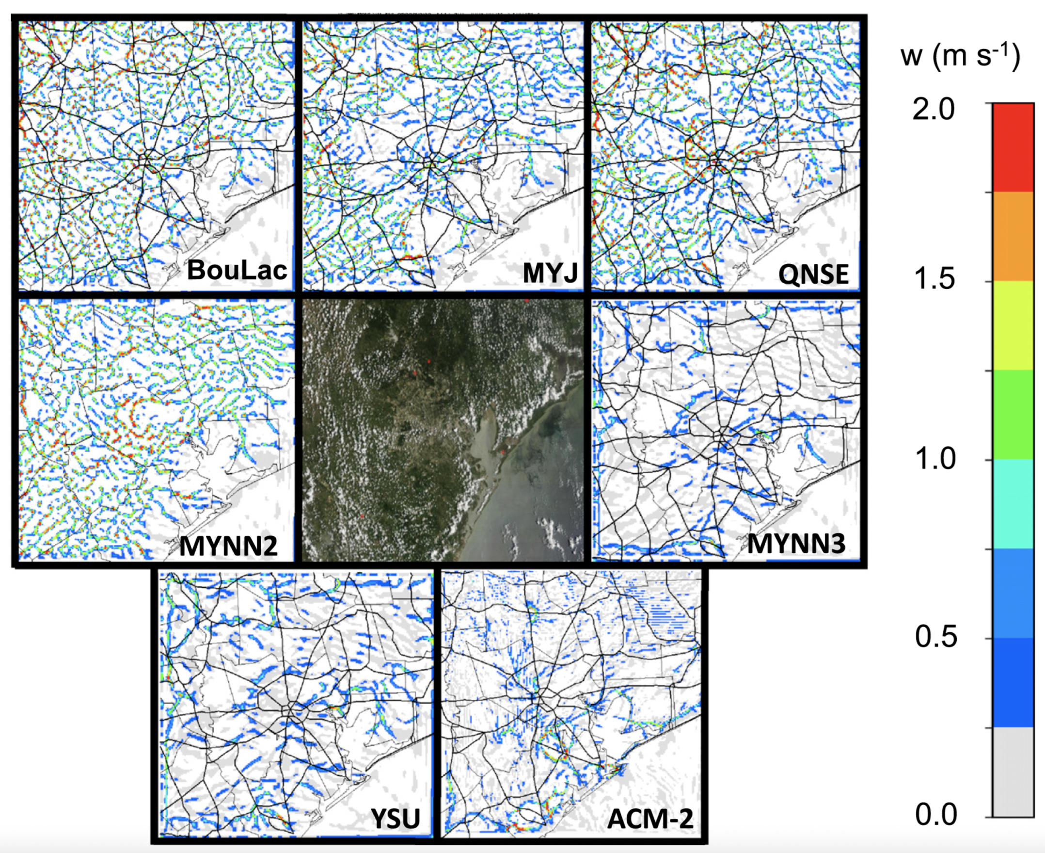
As computational power increases, we are at a time when real-time forecast models for local and regional scales (100–1000 km) are becoming feasible with sub-kilometer grid sizes given that such models have to run at least ten times as fast as real time in operational use. The challenge at these grid scales is that typical convective boundary layer eddies are themselves of scales comparable to the grid and can be considered neither fully resolved nor fully sub-grid, and this puts them in the so-called grey zone or terra incognita. Even at grid sizes near one kilometer, boundary-layer parameterization schemes show a variety of behavior as noted by the Ching et al. study [1] (Figure 1) and [2] as some schemes suppress near-grid-scale cells while others allow them even if they are larger than they should be, and poorly resolved. Some of these schemes also show sensitivity in the range from about 3 km to 1 km grid sizes as they start to permit resolved scale cells only as the grid size reduces which may make their results grid-size dependent.
The role of planetary boundary layer (PBL) schemes in numerical weather prediction models is to transfer heat and moisture fluxes from the surface through the growing boundary layer along with the accompanying surface stress effects on the momentum. In the real atmosphere this is accomplished by large surface-based eddies or thermals with horizontal scales comparable to vertical scales and structures that depend on the heat flux forcing and the shear. Features of these eddies have scales ranging from an order of magnitude less than the PBL depth to a similar scale. From the perspective of models with horizontal grid sizes on the order of kilometers and perhaps 5–10 vertical layers in the lowest kilometer, both typical of weather prediction models, it is essential to represent these sub-grid effects well in order to get a realistic boundary layer growth and mean structure. However, unlike in most of the free atmosphere, this sub-grid effect is not merely passive adiabatic or moist adiabatic and conservative eddy diffusion whereby the vigor of sub-grid mixing is determined by local stability and shear and proportional to gradients of the mixed variables. Instead it is diabatic, driven by energy injected from the surface giving it an active character in which the eddies are modifying the mean profile in a non-conservative way, while providing heat and moisture sources for the convective thermals, the surface also provides a sink for the atmospheric momentum through surface frictional stress.
Representing these as purely sub-grid processes is a challenge that has been met in a variety of successful ways in various PBL schemes, but a further challenge is added in the grey zone as the model dynamics starts to become capable of also resolving some of the transport explicitly with resolved eddies that can result in a competition between resolved transport and sub-grid mixing the outcome of which depends on which is more efficient at removing the instability provided by surface heating. The diverse results of PBL schemes shown by [1] are a result of the various outcomes of this competition.
Another layer of complexity is introduced when there is sufficient moisture for condensation at the tops of the boundary-layer thermals, i.e., shallow convection. In this situation, models have a variety of approaches, but either consider shallow convection as part of the boundary layer thermals, or as a separate process at the top of the boundary layer that may or may not be part of a deep convective parameterization scheme. In the real atmosphere, shallow convection is just part of the boundary-layer thermals, especially if non-precipitating in which case thermodynamic processes are reversible and other conservative thermodynamic quantities can take the place of the potential temperature and water vapor which are no longer conserved in clouds (see Section 5). Seen as an idealized reversible thermodynamic mixing, non-precipitating shallow convection provides no net latent heating as evaporation compensates condensation in a horizontal average sense, so this does not have the large-scale heating effect that precipitating convection has, and consequently drives no large-scale mean vertical motion and convergence.
However, it also needs to be recognized that the presence of clouds introduces stronger radiative effects that may themselves lead to modification of the convective boundary layer eddies, for example top-down mixing induced by the destabilizing effect of longwave radiative cooling at cloud tops. Top-down mixing is also a sub-grid eddy process driven by a different diabatic source that has importance in the evolution of the cloudiness.
2. Large Eddy Simulation and the Grey Zone
First we will address the question of what happens as the grey zone is approached from the high-resolution limit. Typical surface heated boundary layers with vertical scales near 1 km have eddies up to two orders of magnitude smaller that need to be resolved in order that the development of the PBL is fully resolved by the three-dimensional dynamics of the model along with sub-grid eddy mixing that is local and diffusional in character. Characterizing boundary layer development by its heat flux profile and change in depth due to entrainment, converged solutions are seen for grid sizes near 10 m, by which it means that these characteristics are not much altered by going to higher resolutions. This convergence therefore defines a “true” behavior limit that can serve as a baseline from which to gauge problems encountered as the resolution becomes insufficient to represent the key eddy processes. We can use two studies to illustrate how these models start to fail as their grid size becomes too coarse.
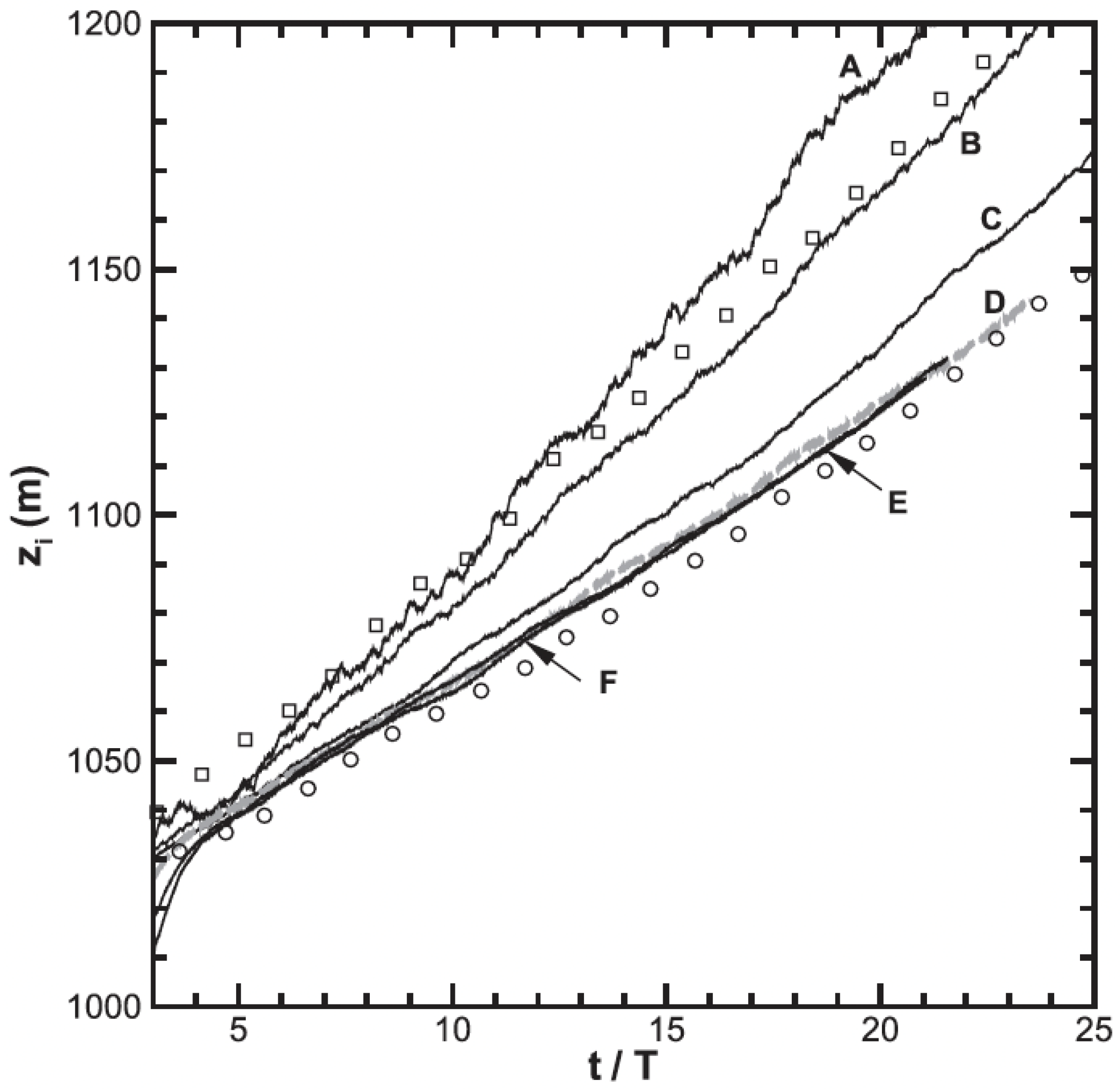
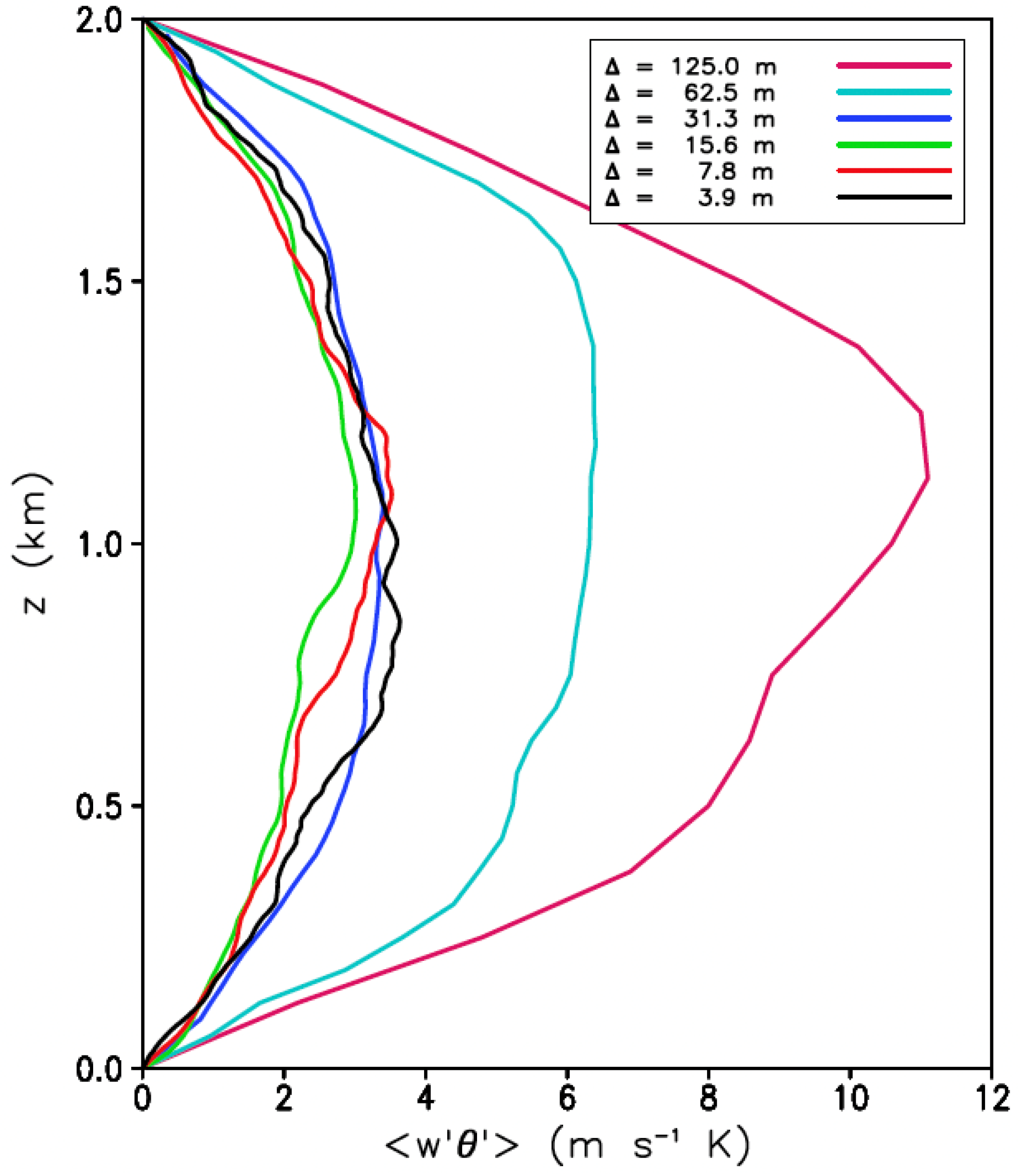
Sullivan and Patton [3] used a set of horizontal grid sizes 5, 10, 20, 40, 80 and 160 m (vertical sizes 40% of horizontal) and examined the PBL growth rate with a fixed surface flux and weak winds. They show that the PBL growth starts to depart from the converged rate at about 40 m grid size, and becomes much faster progressively at 80 and 160 m as seen in Figure 2. A consistent result is shown by Bryan [4] with a different approach using an overturning initially unstable state in a box that also develops convective eddies. Grid sizes used were isotropic at 3.9, 7.8, 15.6, 31.3, 62.5 and 125 m. They showed heat flux profiles (Figure 3) that were converged at high resolutions up to 31.3 m but depart significantly for 62.5 and 125 m when the resolved heat flux becomes much larger.
These studies illustrate the mode of failure as the grid size becomes too coarse to resolve the essential dynamics of the convective eddies. The too-fast growth of the boundary-layer depth and too-large eddy heat flux are consistent with the idea that poorly resolved boundary layer eddies have too little lateral entrainment and retain their undilute properties from low levels too much. The dynamical mixing role of eddies resolved by 10 m grids is not adequately replaced by sub-grid diffusional processes in coarser grids, leaving the larger thermals too strong resulting in both too much heat transport and too much overshooting at the PBL top and consequent entrainment from the free atmosphere above causing the PBL to grow too fast. To compensate for this lack of mixing, the constants used in parameterizing sub-grid eddy terms would have to be increased from standard LES values, or perhaps the vertical sub-grid-scale fluxes need to be enhanced by non-diffusional terms such as proposed by Moeng [5] in representing deep convective eddies in cloud-resolving models. The need to enhance the total vertical flux beyond that which is resolved is certainly clear by the time the grid size exceeds the large-eddy scales and is often considered in PBL parameterizations, as will be seen in the next section.
Another symptom of the failure to resolve is the build-up of energy at the finest resolvable scales in the spectrum which deviates above the slope. These are scales that the model handles poorly and need to be filtered when the natural energy cascade to finer scales is blocked by poor resolution. The necessity of increasing the LES sub-grid mixing parameters at low resolution is also addressed by Takemi and Rotunno [6] in their studies of deep convection at grid sizes near 1 km. Again, this is a compensating measure for the build-up of energy at the poorly resolved scales of the model.
3. PBL Schemes and the Grey Zone
Numerical weather prediction and climate models are not yet able to routinely use LES resolutions and have grid sizes of 1 km to 10 km or more where a PBL parameterization is necessary to represent sub-grid processes that primarily mix heat, moisture and momentum through the boundary layer given surface sources and sinks of these. In the daytime PBL, the eddy fluxes due to thermals are strong even if the mean vertical gradient of the field is weak. There are two primary approaches to this: turbulent kinetic energy prediction local schemes, and enhanced K-profile nonlocal schemes. The latter are referred to as nonlocal because they include terms independent of the local vertical gradients as described later.
Turbulent kinetic energy (tke) prediction is similar to that used in some LES approaches, but only applies to the vertical mixing coefficient because the grid is anisotropic and horizontal mixing applies to relatively larger scales. Many of these schemes follow the Mellor-Yamada closure approach, accounting for buoyancy and shear production and dissipation in the tke equation, and obtain an eddy diffusivity that strengthens with tke.
where is a constant , l is a length-scale and e is the tke. It is an important point that these schemes are still local, so that the subgrid flux depends on the product of the diffusivity and the local vertical gradient of the quantity.
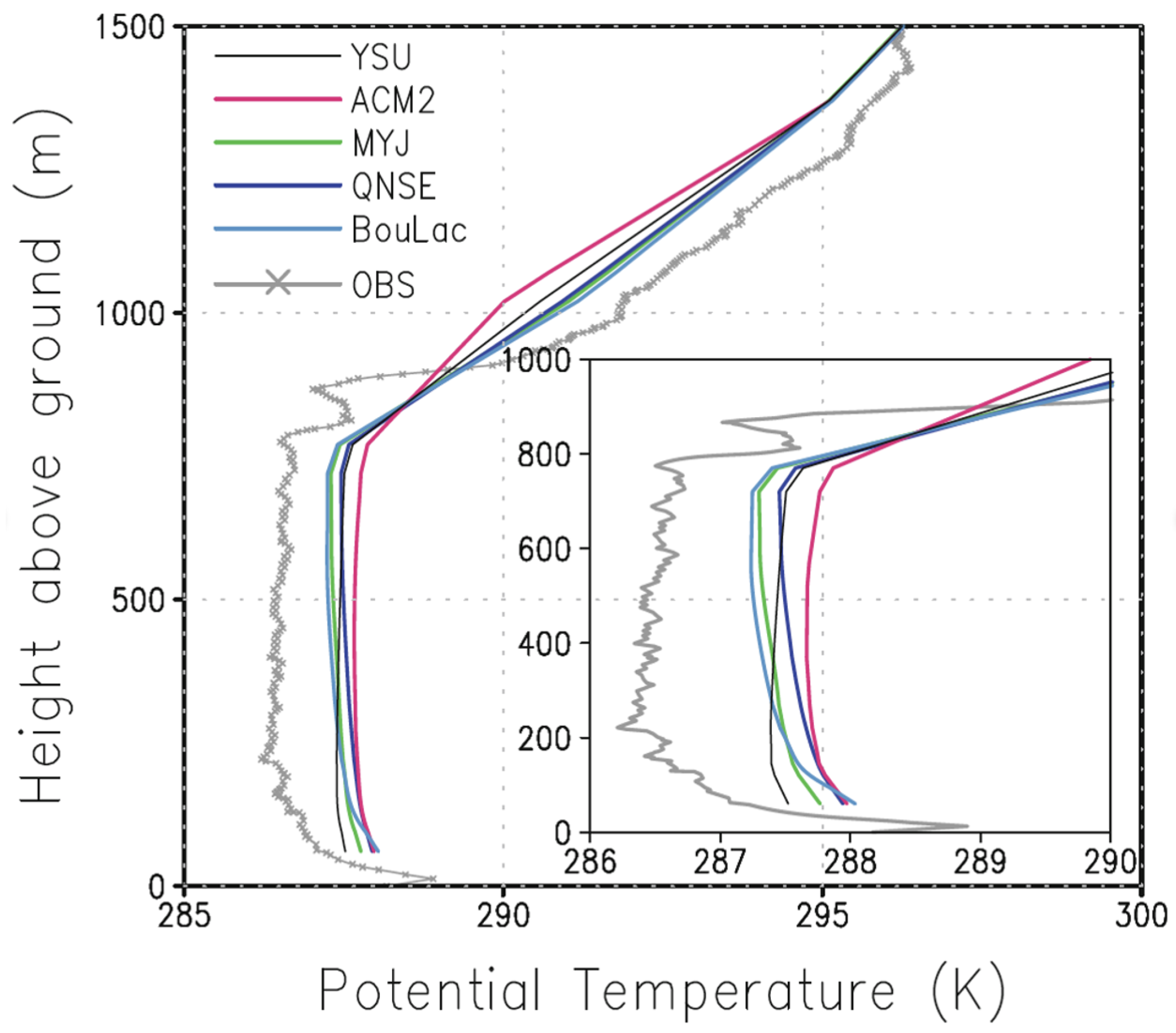
This means that the sub-grid mixing itself is not able to result in the neutral potential temperature profile associated with PBLs, instead remaining slightly superadiabatic as sown by Shin and Hong ([7]. Figure 4 from [7] shows the difference in profiles for three tke schemes (MYJ, QNSE and BouLac) versus two nonlocal schemes (YSU and ACM2) for a grid size of 3 km. However a grid-size dependence of the profile occurs between about 3 km and 1 km in deep boundary layers, as at finer resolutions, the mean profile even of local schemes becomes more neutral. Examining these simulations reveals that at finer resolutions, resolved eddies start to occur that allow for more efficient mixing and neutralizing of the unstable profile (as already seen for these schemes on a 1 km grid in Figure 1), while there were no eddies present at coarser resolutions leaving the mixing completely in the local PBL scheme that requires a resolved gradient for a vertical flux. Even though the tke schemes result in more neutral profiles, it is clear that the resolved energy is larger than it should be, and this was quantified by Shin and Dudhia [8] in comparison with LES using the partitioning methods of Honnert [9]. Later tke schemes have included a nonlocal component in the form of a mass flux due to thermals, e.g., Pergaud [10]. This approach explicitly adds an entraining plume model of transport between the lower and upper PBL that is independent of local vertical gradients.
where represents the combined effects of sub-grid thermal updrafts through the boundary layer and compensating subsidence around them.
A separate branch of evolution of PBL schemes has been to specify the K profile and to include a term that does not depend on the local vertical gradient. The method was made popular by Troen and Mahrt [11] following the ideas of Deardorff [12] whereby a so-called countergradient term () is added to the vertical gradient and both are multiplied by an enhanced K profile peaking in the PBL to produce the vertical sub-grid flux term.
It can be seen that such a term enables a vertical flux even in the absence of a local vertical gradient, and this can result in a neutral to slightly stable potential temperature profile that is more realistic as was seen in Figure 4. The commonly used Yonsei University (YSU) PBL scheme by Hong et al. [13] adopts this method and the term is regarded as a nonlocal mixing term because it is not proportional to the local gradient such as pure diffusion schemes are. With the countergradient method, note that the same K profile is used both for the local and nonlocal strength of vertical flux. As shown by [1,8] schemes with nonlocal mixing tend to suppress resolved eddies even at 1 km grids (Figure 1, YSU and ACM2) where local-diffusion tke schemes allow them. This is because the sub-grid nonlocal transport stabilizes the profile leaving no instability for the resolved scale to remove, unlike the local schemes that leave a resolved superadiabatic profile that allows eddies to grow at fine enough grid sizes. As demonstrated by [1] a similar suppression effect can be achieved by imposing a sufficiently large thermal diffusion guided by critical Rayleigh number considerations.
4. Grey-Zone Schemes
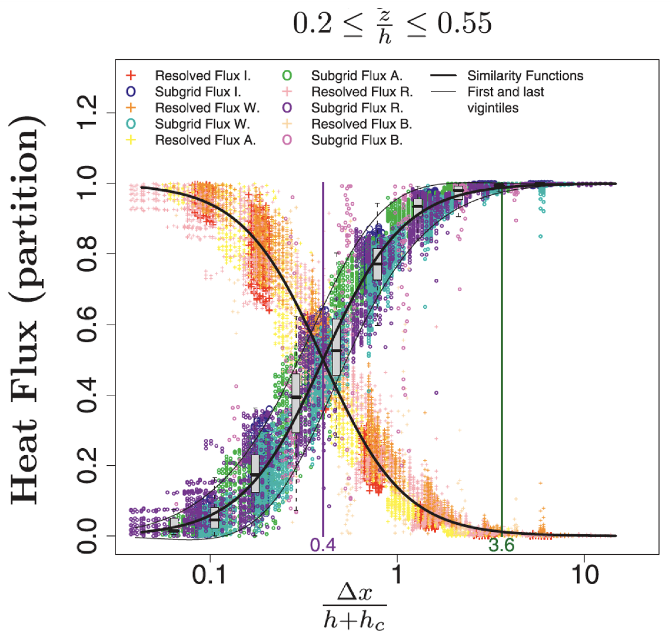
In 2011, a valuable advance was made by Honnert [9] using LES to partition how much of the boundary-layer fluxes should be resolved at each grid size in the grey zone. A fairly universal partitioning function was proposed based on multiple cases where the dependency was on the grid size over the PBL depth (Figure 5).
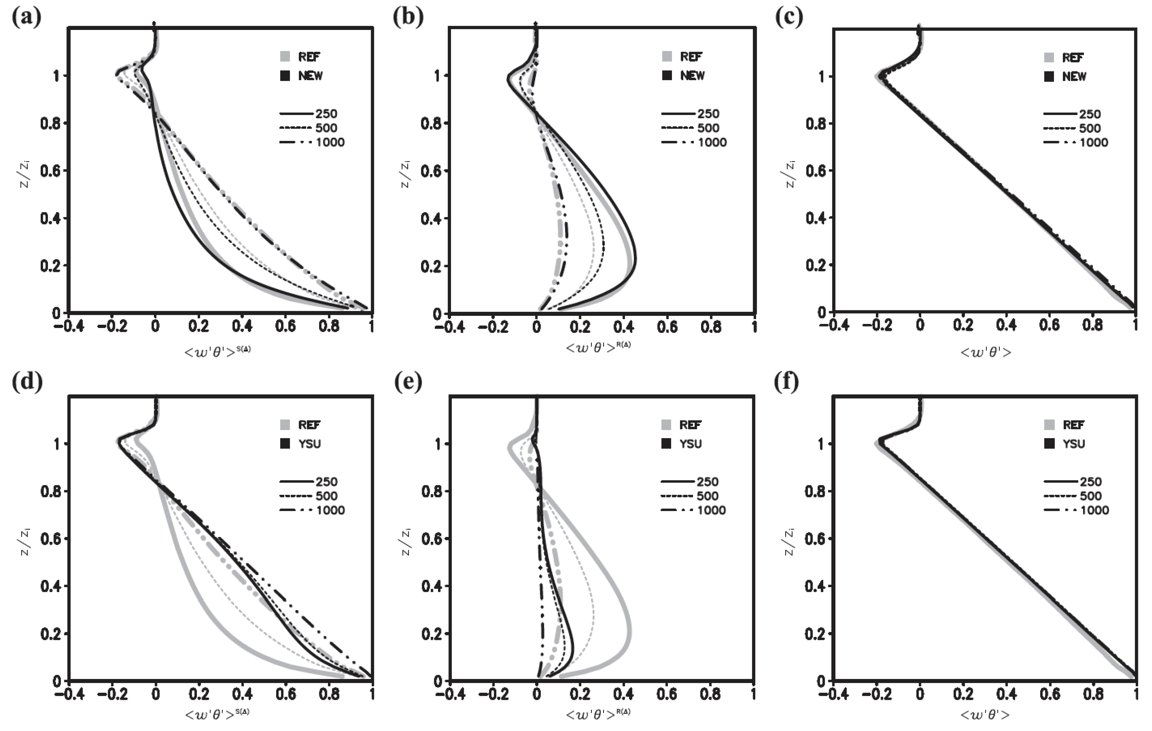
The scale-aware Shin-Hong scheme [14] adapts the strength of the mass-flux term to the grid size in a way designed to partition the energy between resolved and unresolved mixing to be consistent with what can be resolved based on coarsening the grid from LES scales [15], following the methodology of Honnert [9]. The local term retains the K-profile of the YSU PBL scheme but its strength also reduces with grid size to allow more resolved eddies. Figure 6 shows the partitioned subgrid-scale (left column) and resolved fluxes (middle column) for the scale-aware scheme (upper panels) and non scale-aware YSU scheme (lower panels) for three different grid sizes across the grey zone together with the reference LES solution partitioning (grey lines). The right column shows that the improved partitioning does not change the total flux, but this scheme does give more grid-consistent varying eddy strengths across the grey zone, while being scale aware, this scheme does not become a traditional LES scheme in the fine-scale limit as the vertical mixing remains decoupled from the horizontal mixing similarly to all one-dimensional PBL schemes.
One of the first schemes that enabled transitioning from a PBL approach with a nonlocal mass flux to a fully 3d Smagorinsky sub-grid turbulence approach using Honnert’s methodology was Boutle et al. [16]. The 3d mixing at the small scale limit depends on horizontal grid size, vertical shear and Richardson number, making it more similar to cloud-model and free-atmosphere sub-grid mixing than the more isotropic approach used in most LES models.
Meanwhile Ito et al. [17] derived similar scaling functions to reduce length scales from the Level 3 Mellor-Yamada-Nakanishi-Niino ([18]) mesoscale PBL scheme to a scale-aware scheme as the grid size transitions below the mesoscale limit, which is generally where it is less than the PBL depth. The Level 3 closure allows countergradient fluxes using a local closure as opposed to explicit non-gradient flux terms.
Building on the Shin-Hong and Honnert methodology, Zhang et al. [19] developed a three-dimensional scale-aware PBL scheme called 3dTKE that fully reverts to the LES sub-grid model at grid sizes much less than 0.1 where is the PBL height. This includes the non-local mass flux profile of Shin-Hong and scaling terms for this along with vertical and horizontal diffusion between LES and mesoscale limits in the grey zone. Being a tke scheme, in contrast to Shin-Hong, the tke equation is also made scale aware using a length scale with mesoscale and LES limits using the mesoscale limit of the MYNN (Mellor-Yamada and Nakanishi-Niino) PBL scheme ([18]).
5. Cloud-Topped Boundary Layers
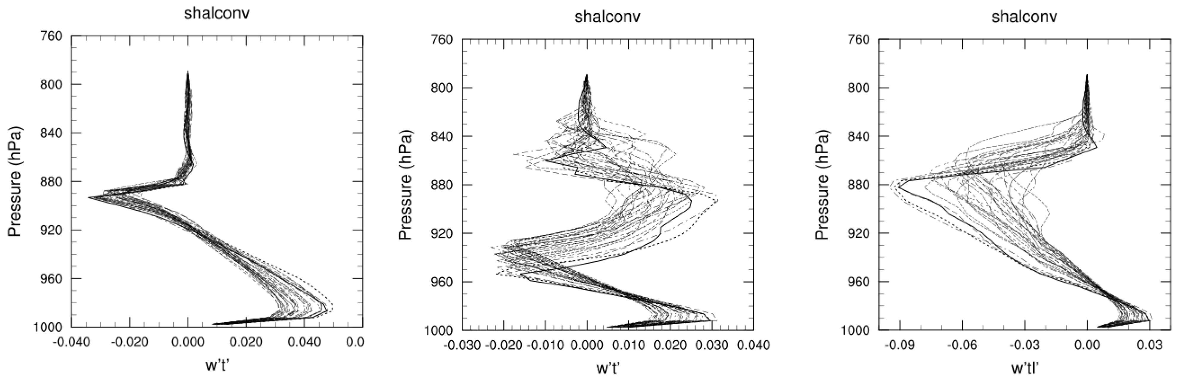
Up until this point, this review has focused on the challenges of representing the dry boundary layer at sub-kilometer resolutions. Very often boundary layers do not remain dry throughout their development as saturation occurs in the rising thermals with latent heat release strongly modifying the effective stability, while the clouds do not precipitate, idealized cloud-topped boundary layers can still be considered to have reversible thermodynamics, and conservative properties can be defined that take the place of potential temperature and water vapor, such as moist static energy, liquid water potential temperature and total moisture (cloud plus vapor). This is illustrated for a large-eddy simulation case at 100 m grid size where the resolved vertical eddy flux of potential temperature when shallow convection occurs is complicated by the condensation source that enhances it in the lower cloud. However the vertical eddy flux of liquid water potential temperature () is much simpler and more similar to the dry case with an enhanced entrainment layer of negative correlation (Figure 7).
In models, this process is handled as shallow convection in a variety of ways. The shallow convection may be part of a deep convection scheme in which the same methods are used as for deep clouds, often a mass-flux approach, but modified for smaller radius, strongly entraining, non-precipitating clouds with low tops. Alternatively shallow convection may have a stand-alone parameterization that activates based on moist instability at the top of the existing dry boundary layer that is independently parameterized. Or, in what may be a preferable approach, the boundary-layer scheme allows for condensation within its parameterized thermals in a more unified way of handling them from the surface through cloud top. The latest advances in this area include eddy-diffusion mass-flux (EDMF) schemes with multi-plume approaches following Neggers [20] wherein a population of plumes with different radii, and hence entrainments, represents the sub-grid mass flux transport. A scale-aware application may vary the number and size of these sub-grid thermals Angevine et al. [21].
We can also note that even if a dry boundary-layer parameterization is used without shallow convection its growth can reach saturation at the lifting condensation level in which case resolved clouds are produced by the cloud condensation scheme stabilizing the air relative to the dry PBL so that the PBL top remains near cloud base. The in-cloud subgrid vertical mixing should also be sensitive to moist adiabatic unstable layers, rather than the dry adiabatic lapse rate, and enhance local vertical mixing in such layers so that realistic thermodynamic profiles may be achieved. Or the dry PBL approach can be modified to use conserved quantities, liquid water potential temperature and total moisture, in which case its depth becomes insensitive to cloud base due to the continuity of the profiles of these variables across that level. This would lead to a deeper defined PBL height that includes the shallow cloud layer, but still requires a condensation adjustment to take place on the resulting profile.
As mentioned in the Introduction, while cumulus clouds can be thought of as part of the surface-based boundary-layer eddies with reversible thermodynamics in an idealized sense, in reality the radiative interaction with cloud tops can drive separate top-down mixing through long-wave cooling resulting in more complex boundary layer structures such as may be seen with marine stratocumulus.
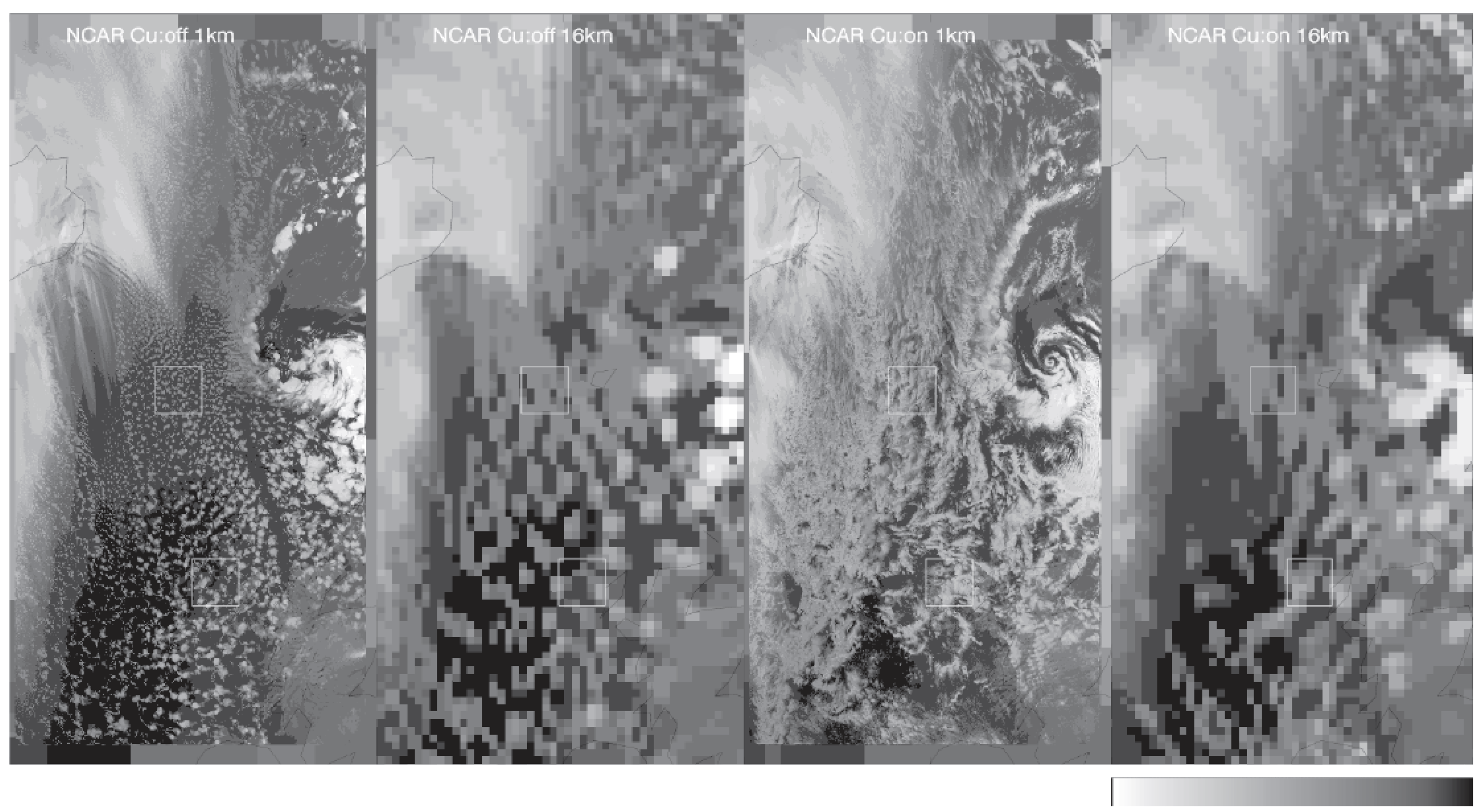
The deepening of shallow clouds also extends the grey-zone for parameterizations beyond 1 km. An international study by Field et al. [22] compared several models at resolutions between 1 and 16 km with and without convective parameterizations for an ocean cold-air outbreak case. They found that the stratocumulus regime was challenging for this range of grid sizes while the more convective regime with larger cells showed signs of convergence at higher resolution which is consistent with the scales of the main eddies. An example from one model (WRF) for OLR is shown at 1 km and 16 km without and with a deep cumulus scheme is shown in Figure 8.
6. Concluding Remarks
The aim of this paper has not been to give a thorough review of all research in this challenging area of modeling the atmospheric boundary layer, but to give a perspective on what happens in models at these scales by summarizing selected relevant work with the specific aim of illustrating the primary problems and solutions with a limited level of detail to keep the article concise while addressing a broad range of related topics. The hope is that this has shed light on what physical processes need to be represented well and what happens if they are not. Boundary-layer eddies are not fully resolved unless the grid size is a few tens of meters, and large-eddy models resolving these scales have become very informative on how the grey zone should be treated. Numerical weather prediction models are only now reaching sub-kilometer grids and starting to show some divergent behavior depending on how their boundary-layer parameterization schemes are formulated. This was well illustrated by the Ching study [1] as mentioned in the Introduction, and here we build on their work, by providing additional perspectives gained from large-eddy studies and the development of new grey-zone parameterizations in recent years. The paper ends by briefly touching on the added complications of shallow cumulus-topped boundary layers, but makes the case that a unified approach to boundary-layer eddies whether cloud-topped or not is a physically-based reasonable goal. Cloud-topped boundary layers expand the grey zone to kilometer scales as the eddy widths scale with the height, and clouds also introduce radiative interactions as a first-order contribution to the stability and dynamics.
We have not addressed complex topography or the stable boundary layer that introduce additional surface complexities. Achieving a reasonable diurnal cycle in surface wind requires accounting for sub-grid drag effects differently in stable and unstable conditions as shown by Jimenez et al. [23,24]. The vertical scales in the stable boundary layer are typically small compared to model resolutions, and there may be a surface mixed layer up to a few tens of meters with a depth controlled by the ambient wind seen in the observational studies of Sun et al. [25], or drainage flows resulting from surface cooling in combination with small-scale topographic gradients. Thus, in contrast to the convective boundary layer, the stable boundary layer will remain a part of sub-grid-scale parameterization schemes.
Funding
This research received no external funding.
Acknowledgments
The author has benefited from many practical discussions of these issues with numerous colleagues and would especially like to mention Hailey Shin, Pedro Jimenez and Songyou Hong who collaborated on work that provided some insights mentioned in this review. This work is supported by the National Center for Atmospheric Research, which is a major facility sponsored by the National Science Foundation under Cooperative Agreement No. 1852977.
Conflicts of Interest
The author declares no conflict of interest.
References
- Ching, J.; Rotunno, R.; LeMone, M.A.; Martilli, A.; Kosovic, B.; Jimenez, P.; Dudhia, J. Convectively induced secondary circulations in fine-grid mesoscale numerical weather prediction models. Mon. Weather Rev. 2014, 142, 3284–3302. [Google Scholar] [CrossRef] [Green Version]
- Zhou, B.; Simon, J.S.; Chow, F.K. The convective boundary layer in the terra incognita. J. Atmos. Sci. 2014, 71, 2545–2563. [Google Scholar] [CrossRef]
- Sullivan, P.P.; Patton, E.G. The effect of mesh resolution on convective boundary layer statistics and structures generated by large-eddy simulation. J. Atmos. Sci. 2011, 68, 2395–2415. [Google Scholar] [CrossRef] [Green Version]
- Bryan, G.H.; Rotunno, R. Statistical convergence in simulated moist absolutely unstable layers. In Proceedings of the 11th Conference on Mesoscale Processes, Albuquerque, NM, USA, 24–29 October 2005; American Meteorological Society: Albuquerque, NM, USA, 2005. [Google Scholar]
- Moeng, C.-H. A closure for updraft–downdraft representation of subgrid-scale fluxes in cloud-resolving models. Mon. Weather Rev. 2014, 142, 703–715. [Google Scholar] [CrossRef]
- Takemi, T.; Rotunno, R. The effects of subgrid model mixing and numerical filtering in simulations of mesoscale cloud systems. Mon. Weather Rev. 2003, 131, 2085–2101. [Google Scholar] [CrossRef]
- Shin, H.H.; Hong, S.-Y. Intercomparison of planetary boundary-layer parametrizations in the WRF model for a single day from CASES-99. Bound.-Layer Meteorol. 2011, 139, 261–281. [Google Scholar] [CrossRef]
- Shin, H.H.; Dudhia, J. Evaluation of PBL parameterizations in WRF at sub-kilometer Resolution: Turbulence statistics in the convective boundary layer. Mon. Weather Rev. 2016, 144, 1161–1177. [Google Scholar] [CrossRef]
- Honnert, R.; Masson, V.; Couvreux, F. A diagnostic for evaluating the representation of turbulence in atmospheric models at the kilometric scale. J. Atmos. Sci. 2011, 68, 3112–3131. [Google Scholar] [CrossRef]
- Pergaud, J.; Masson, V.; Malardel, S.; Couvreux, F. A parameterization of dry thermals and shallow cumuli for mesoscale numerical weather prediction. Bound.-Layer Meteorol. 2009, 132, 83–106. [Google Scholar] [CrossRef]
- Troen, I.; Mahrt, L. A simple model of the atmospheric boundary layer; sensitivity to surface evaporation. Bound.-Layer Meteorol. 1986, 37, 129–148. [Google Scholar] [CrossRef]
- Deardorff, J.W. Parameterization of the planetary boundary layer for use in general circulation models. Mon. Weather Rev. 1972, 100, 93–106. [Google Scholar] [CrossRef]
- Hong, S.-Y.; Noh, Y.; Dudhia, J. A new vertical diffusion package with an explicit treatment of entrainment processes. Mon. Weather Rev. 2006, 134, 2318–2341. [Google Scholar] [CrossRef] [Green Version]
- Shin, H.H.; Hong, S.-Y. Representation of the subgrid-scale turbulent transport in convective boundary layers at gray-zone resolutions. Mon. Weather Rev. 2015, 143, 250–271. [Google Scholar] [CrossRef]
- Shin, H.H.; Hong, S.-Y. Analysis of resolved and parameterized vertical transports in convective boundary layers at gray-zone resolutions. J. Atmos. Sci. 2013, 70, 3248–3261. [Google Scholar] [CrossRef]
- Boutle, I.A.; Eyre, J.E.J.; Lock, A.P. Seamless stratocumulus simulation across the turbulent gray zone. Mon. Weather Rev. 2014, 142, 1655–1668. [Google Scholar] [CrossRef]
- Ito, J.; Niino, H.; Nakanishi, M.; Moeng, C.-H. An extension of Mellor–Yamada model to the terra incognita zone for dry convective mixed layers in the free convection regime. Bound.-Layer Meteorol. 2015, 157, 23–43. [Google Scholar] [CrossRef]
- Nakanishi, M.; Niino, H. Development of an improved turbulence closure model for the atmospheric boundary layer. J. Meteorol. Soc. Jpn. 2009, 87, 89–912. [Google Scholar] [CrossRef] [Green Version]
- Zhang, X.; Bao, J.-W.; Chen, B.; Grell, E.D. A three-dimensional scale-adaptive turbulent kinetic energy scheme in the WRF-ARW model. Mon. Weather Rev. 2018, 146, 2023–2045. [Google Scholar] [CrossRef]
- Neggers, R.A.J. Exploring bin-macrophysics models for moist convective transport and clouds. J. Adv. Model. Earth Syst. 2015, 7, 2079–2104. [Google Scholar] [CrossRef] [Green Version]
- Angevine, W.A.; Olson, J.; Kenyon, J.; Gustafson, W.I.; Endo, S.; Suselj, K.; Turner, D.D. Shallow cumulus in WRF parameterizations evaluated against LASSO large-eddy simulations. Mon. Weather Rev. 2018, 146, 4303–4322. [Google Scholar] [CrossRef]
- Field, P.R.; Brozkova, R.; Chen, M.; Dudhia, J.; Lac, C.; Hara, T.; Honnert, R.; Olson, J.; Siebesma, P.; de Roode, S.; et al. Exploring the convective greyzone with regional simulations of a cold air outbreak. Q. J. R. Meteorol. Soc. 2017, 143, 2537–2555. [Google Scholar] [CrossRef] [Green Version]
- Jimenez, P.A.; Dudhia, J. Improving the representation of resolved and unresolved topographic effects on surface wind in the WRF model. J. Appl. Meteorol. Clim. 2012, 51, 300–316. [Google Scholar] [CrossRef] [Green Version]
- Lorente-Plazas, R.; Jimenez, P.A.; Dudhia, J.; Montavez, J.P. Evaluating and improving the impact of the atmospheric stability and orography on surface winds in the WRF model. Mon. Weather Rev. 2016, 144, 2685–2693. [Google Scholar] [CrossRef]
- Sun, J.; Mahrt, L.; Banta, R.M.; Pichugina, Y.L. Turbulence regimes and turbulence intermittency in the stable boundary layer during CASES-99. J. Atmos. Sci. 2012, 69, 338–351. [Google Scholar] [CrossRef]
Figure 1.
From Ching et al. [1]. Comparison of observed PBL-generated clouds to positive vertical velocity (w) at 125 m (level 10) for 2000UTC4 August 2006 over the Houston–Galveston area using various PBL schemes in WRF at 1-km grid spacing. Satellite image, Terra, 1720 UTC, 500-m pixels in center. For the PBL schemes shown, vertical fluxes are proportional to local vertical gradients for BouLac, MYJ, QNSE, and MYNN2; while nonlocal vertical fluxes (independent of local vertical gradients) are also allowed for MYNN3, YSU, and the asymmetric cloud model version 2 (ACM-2) ©American Meteorological Society. Used with permission.

Figure 2.
From Sullivan and Patton [3]. Variation of the boundary layer height with nondimensional time ; the large-eddy time scale . The labels A–F correspond to the grid resolutions 160, 80, 40, 20, 10 and 5 m, respectively. The high-resolution runs (D–F) overlap. The simulation marked with an open square uses a mesh of 643 but with no monotone vertical temperature flux; that marked with an open circle uses a mesh of 20 m and is identical to simulation D but uses a filter width equal to simulation B. ©American Meteorological Society. Used with permission.

Figure 3.
From Bryan [4]. Vertical profiles of vertical temperature flux from all simulations at the time of maximum flux.
Figure 3.
From Bryan [4]. Vertical profiles of vertical temperature flux from all simulations at the time of maximum flux.

Figure 4.
From Shin and Hong [7]. Vertical profile of the simulated potential temperature (K), at 1900 UTC 23 October (1400 LST 23 October) with corresponding radiosonde soundings (grey lines with cross marks). The simulated results are from the YSU (black), ACM2 (red), MYJ (green), QNSE (blue), and BouLac (light blue) experiments. The inset provides a closer look at the temperature profiles in the lowest 1000 m. Reprinted by permission from Springer Nature, Boundary-Layer Meteorology, ©2011.

Figure 5.
From Honnert et al. [9]. Partition of the resolved heat flux (crosses; IHOP: red, Wangara: orange, AMMA: yellow, ARM: pink, BOMEX: wheat) and subgrid heat flux (circles; IHOP: blue, Wangara: cyan, AMMA: green, ARM: purple, BOMEX: violet) as a function of the dimensionless mesh: in the Mixing Layer. In the legend, I. means IHOP, A. means AMMA, W. means Wangara, B. means BOMEX, and R. means ARM. The vertical purple line represents the scale for which subgrid and resolved heat have the same value. The black lines represent the partial similarity functions. The vertical dark green line is the scale for which the total heat flux is more than 95% subgrid. The gray box-and-whiskers plots summarize the median and the variance of the resolved data per class of . The fine black lines on both sides of the similarity functions are the first and the last vigintiles of the data. ©American Meteorological Society. Used with permission.

Figure 6.
From Shin and Hong [14]. For buoyancy and wind forced case, domain-averaged (a,d) subgrid-scale (SGS); (b,e) resolved; and (c,f) total vertical heat transport profiles for (top) NEW and (bottom) YSU experiments (black) with corresponding REF profiles (gray): 250 m (solid), 500 m (dotted), and 1000 m (dot–dot–dashed). ©American Meteorological Society. Used with permission.

Figure 7.
Vertical mean profiles at various times of simulation of (left) eddy potential temperature flux in a dry boundary layer, (center) eddy potential temperature flux in a cloud-topped boundary layer, and (right) eddy liquid-water potential temperature flux in the same cloud-topped boundary layer.

Figure 8.
From Field et al. [22]. Top of atmosphere outgoing long-wave fluxes from NCAR model from a 24 h forecast valid for 1200 UTC 31 January 2010. From left to right, 1 km convection off, 1 km convection on, 16 km convection off, 16 km convection on. Reprinted by permission from John Wiley and Sons, Quarterly Journal of the Royal Meteorological Society, ©2017.

Publisher’s Note: MDPI stays neutral with regard to jurisdictional claims in published maps and institutional affiliations. |
© 2022 by the author. Licensee MDPI, Basel, Switzerland. This article is an open access article distributed under the terms and conditions of the Creative Commons Attribution (CC BY) license (https://creativecommons.org/licenses/by/4.0/).
Share and Cite
MDPI and ACS Style
Dudhia, J. Challenges in Sub-Kilometer Grid Modeling of the Convective Planetary Boundary Layer. Meteorology 2022, 1, 402-413. https://doi.org/10.3390/meteorology1040026
AMA Style
Dudhia J. Challenges in Sub-Kilometer Grid Modeling of the Convective Planetary Boundary Layer. Meteorology. 2022; 1(4):402-413. https://doi.org/10.3390/meteorology1040026
Chicago/Turabian StyleDudhia, Jimy. 2022. "Challenges in Sub-Kilometer Grid Modeling of the Convective Planetary Boundary Layer" Meteorology 1, no. 4: 402-413. https://doi.org/10.3390/meteorology1040026