1. Introduction
Modern cosmology is a dynamic interplay of theoretical and experimental endeavors, continually evolving to surmount novel challenges. The discipline necessitates systematic reconstruction to harmonize theory with emerging observational data at each juncture. A watershed moment in this ongoing debate unfolded with the revelation of supernova dimming [
1], a phenomenon that revealed the limitations of the Friedmann–Lemaitre–Robertson–Walker metric (herein Friedmann metric). To address this dissonance, the cosmological constant was introduced to align the theoretical predictions with empirical insights [
2].
Contemporary surveys and astronomical observations indicate that galaxies are increasingly moving away from us. At the core of current cosmological discussions is the significant challenge of understanding the formation of structures and the evolution of galaxies amidst the backdrop of the accelerated expansion in the late-time universe. The Friedmann model, rooted in the cosmological principle, has effectively described the universe’s evolution in line with empirical observations [
3,
4,
5,
6]. However, the mystery of dark energy and the force driving cosmic acceleration remains a persistent challenge in contemporary physical cosmology [
7,
8].
Various attempts to explain cosmic acceleration rely on concepts such as the cosmological constant or scenarios dominated by dark energy. However, the perplexities surrounding the cosmological constant pose significant puzzles [
9,
10,
11]. Adding to these difficulties is the potential violation of the cosmological principle when homogeneity or isotropy falters in galaxy structure formation [
12,
13].
As for three-dimensional redshift, surveys delve deeper into the cosmos, revealing structures lacking a transition to homogeneity [
14,
15,
16,
17]; questions arise regarding the steadfastness of the cosmological principle. The galaxy distribution in recent observations (light) and the simulation of dark matter distribution (matter) display significant inhomogeneity on the largest statistical scale available. The matter distribution exhibits even greater inhomogeneity, challenging the search for the cosmological principle in the current observed light or matter distribution in the universe [
18]. Recent studies on the angular scale of cosmic homogeneity using the Sloan Digital Sky Survey’s Sixteenth Data Release (SDSS-IV DR16) of a luminous red galaxy sample based on a model-independent approach found a homogeneity of 60–80 h
−1 Mpc [
19]. This finding was recently challenged through a homogeneity test for the matter distribution based on the Baryon Oscillation Spectroscopic Survey Data Release 12 CMASS galaxy sample [
20]. It was found that the observed distribution of matter is statistically unlikely to be a random arrangement up to a radius of 300 h
−1 Mpc, which is approximately the largest statistically available scale [
18].
The identification of large quasar groups (LQGs) further catalyzes the debate, suggesting an inherent inhomogeneity incompatible with prevailing cosmological paradigms [
21,
22,
23]. Such revelations underscore the need for a profound cosmological reassessment. Correct testing on the prediction of the standard model on the spatial distributions of luminous astronomical sources needs to be based on cosmological simulations of a high resolution involving a large sample of isolated galaxies using robust data-driven detectors to avoid misinterpretations of the analyzed sources [
24].
While two-dimensional projections appear consonant with isotropy and homogeneity, three-dimensional catalogues unveil a complex picture of inhomogeneous galactic distributions. These divergent findings regarding the transition to homogeneity confound attempts at a unified perspective [
25,
26,
27].
The contrasting nature of these observations challenges the conventional assumption of cosmic homogeneity and isotropy. The implications have a potential impact on understanding cosmic acceleration and the need for an additional dark energy component [
13,
28,
29]. Researchers find it necessary to explore alternative models of dark energy or its modified forms to account for the cosmic acceleration of the universe, considering the observational anomalies of the standard model and its lack of physical motivation [
30,
31,
32,
33]. The proposed model includes scenarios where the scalar field replaces the cosmological constant to represent dark energy and modified gravity theories [
34,
35].
Recent observations, such as the unexplained Hubble parameter tensions, large-scale anisotropies, and massive disk galaxies at higher redshifts, pose challenges to the Friedmann model and the concordance model of cosmology in general. For example, the Hubble parameter determined from the cosmic microwave background (CMB) radiation differs from that determined using Type Ia supernovae and the redshift of their host galaxies [
33,
36,
37]. While one possible explanation is the incompleteness of the concordance model, alternative theories propose that the standard redshift model, as a distance–scale factor relation, might be incomplete [
38]. Addressing these observations supports modifications to some foundations of cosmology based on the cosmological principle [
39]. Modifying the standard redshift relation may offer a plausible explanation for investigating recent Hubble tensions [
38].
Some other models propose cosmic acceleration as an emergent phenomenon [
40,
41,
42]. The fundamental effect of cosmic evolution on photon propagation is cosmological redshift. In the standard model, cosmological redshift is a theoretical function of the scale factor derived from the Friedmann metric. However, researchers are now reconstructing this scale factor–redshift relation from observations rather than relying on its theoretical form [
40,
41,
42].
One drawback of remapping cosmological models is the unknown function of the observed redshift, increasing the degree of freedom of the equation. This issue has been addressed by introducing function parameterization through Taylor expansion before adopting a parametric approach. Related work includes a cosmological model proposed to explain the accelerated expansion of the universe by modifying the standard redshift relation [
31]. It has been demonstrated that combining Friedmann equations with a modification of redshift remapping may lead to a self-consistent framework under the assumption of the inadequacy of the Friedmann model [
42,
43]. The parametric [
40], non-parametric [
42], and modified standard redshift models [
31] are expected to address the cosmological constant problem.
However, all these ambitious objectives hinge upon an indispensable prerequisite—an abundance of accurate and expansive cosmological data. Despite the growing body of observational data, persistent limitations require a careful interpretation of the current cosmological models’ completeness and accuracy [
36,
44,
45,
46]. The upcoming Vera Rubin Observatory holds the potential for a transformative ten-year exploration, armed with a 3.6 Gigapixel camera, ready to survey the entire visible night sky and delve into cosmic intricacies [
47].
Given the unsettling findings discussed above, there is a widespread unease regarding the validity of current cosmological models. To address this concern, we introduce a modified redshift Friedmann model that is tuned to the distribution of luminous matter in the universe. This study focuses on three key astronomical parameters: number density, light intensity, and redshift. We investigate the evolution of number density and light intensity with redshift in both the standard redshift Friedmann model and its proposed modified version. Our analysis carefully considers the impact of dark matter and dark energy within these models.
The paper is structured as follows:
Section 2 introduces pertinent models relevant to our work, while
Section 3 illuminates our analytical findings.
Section 4 engages in the simulation and discussion of these findings, and the paper culminates in
Section 5 with definitive conclusions.
2. Background Model Formulation
2.1. Parametric Model
The parametric model proposed by Bassett et al. [
40] in 2015 introduces modifications to the traditional redshift paradigm, seeking to refine our understanding of cosmic dynamics. This model involves the introduction of parameters that capture modifications in the redshift space, allowing for a more nuanced interpretation of observational data. The model addresses subtle aspects of cosmic phenomena by incorporating specific parameters, providing a more detailed and accurate representation of redshift-related observations.
2.2. Non-Parametric Model
The non-parametric model, as formulated by Wojtak and Prada [
42] in 2017, takes a distinct approach by avoiding predefined parameters, allowing for greater flexibility in modeling cosmic phenomena. Unlike parametric models, the non-parametric model refrains from imposing fixed parameters, enabling a more adaptive and data-driven analysis of redshift-related phenomena.
This model is precious in scenarios where the underlying dynamics are complex and not easily encapsulated by predefined parameters. It provides a more versatile tool for interpreting observational data.
The above two models proposed by [
40,
42] and used in this paper contribute to different perspectives on how redshift modifications can enhance our understanding of the universe. While the parametric model introduces specific parameters, the non-parametric model adopts a more flexible and adaptive approach, catering to the intricacies of cosmic dynamics.
2.3. The Friedmann Model
Consider the Einstein field equations in the form:
Here, is the Einstein tensor, which is computed from the metric tensor , is the Ricci tensor, is the Ricci scalar, is the cosmological constant representing the dark energy component, is the energy momentum tensor characterizing matter distribution, and = where G is the gravitational constant and is the speed of light.
Consider also the Friedmann–Lemaitre–Robertson–Walker spacetime metric for a universe that is filled with homogeneous and isotropic matter:
Here, being the scale factor of the universe representing the time-dependent evolution of the spatial part of the metric on surfaces of constant time , and , determines the geometry of these spatial sections as non-flat and flat, respectively.
Derivations involving Equations (1) and (2) yield two Friedmann equations for describing the relativistic dynamics and evolution of the universe (see details of calculations in [
48], expressed as:
and
Here, the single and double overhead dots denote the first and second derivatives with respect to time t, respectively; is the space curvature geometry with values or , is the pressure, and is the density of the universe both expressed as functions of time .
Equations (3) and (4) have been demonstrated [
48,
49] to yield:
The left-hand side of this equation represents the rate of change of the total energy in the universe. In the matter-dominated cosmology, where the main energy density is in cold, with non-relativistic matter behaving like dust (i.e.,
), Equation (5) simplifies to
Equation (6) indicates that the total mass contained in the universe remains constant, aligning with the relativistic theory of matter and fields (Noether’s theorem), where there is no preferred direction for the motion of matter to maintain isotropy.
Equation (6) can be reformulated as [
48,
49]:
Equation (7) represents the time taken for a light photon to travel at a distance = , describing a matter-dominated Friedmann universe. Friedmann Equations (3) and (4) in the form of Equation (7) will later be employed in this paper to derive the light intensity–modified redshift and number density–modified redshift relations.
2.4. Modified Redshift Model
Redshift scale factor modifications offer a promising approach, presenting a novel perspective on the dynamics of the universe. Cosmic expansion’s acceleration remains a key cosmological puzzle [
7]. Redshift scale factor modifications provide a unified framework, addressing both early-time inflationary expansion and late-time cosmic acceleration. This unity eliminates the need for distinct mechanisms across different epochs, offering a more cohesive picture of the universe.
These modifications effectively account for large-scale structures and the cosmic microwave background, maintaining consistency with cosmological observations.
The elusive nature of dark energy, responsible for cosmic acceleration, finds a more tangible alternative in redshift scale factor modifications. By incorporating these changes, we may gain deeper insights into the mechanisms behind cosmic acceleration.
The introduction of redshift scale factor modified relations may also have implications for fundamental physics. Revisiting the universe’s dynamics on a large scale may unveil connections between cosmological observations and the behavior of matter and energy at the most fundamental levels.
Therefore, the incorporation of modified redshift scale factor relations into cosmological models presents a compelling and physically plausible avenue for advancing our understanding of the universe and offers a fresh perspective that may help resolve existing anomalies and contribute to a complete and more coherent cosmological framework.
In this work, we undertake an examination of a modified redshift relation to scrutinize the relativistic dynamics and structure formation in a matter-dominated Friedmann universe. Our methodology involves the incorporation of a modified version of the standard redshift relation, as introduced by [
31], into the Friedmann equations. The model [
31] is succinctly outlined as follows:
The conventional correlation between cosmological redshift and the cosmic scale factor for light photons is expressed as
Hereafter referred to as the standard redshift relation. Should we posit that unknown quantum effects exert a discernible influence on the frequency of light photons during their cosmological propagation, then the aforementioned relation can be altered to
It is discernible from the modified redshift equation that when = , the equation reverts to its standard form. Consequently, the modified equation, being more generalized, is anticipated to yield more comprehensive results upon the appropriate specification of . This enhancement goes beyond classical experimental tests that aim to distinguish between the metric and non-metric origins of the cosmological redshift.
We shall proceed to fit the derived Friedmann equations using parametric equation [
40]:
where
and
are arbitrary parameters and non-parametric [
42] (modified redshift functions;
where
is a freely varying function of
. The parameter values in these models are constrained through standard observational datasets to deduce the optimal present values of cosmological parameters. Notably, these models, grounded in the redshift-scale-factor-remapping concept, exhibit consistency with contemporary astronomical observations [
42]. We introduce slight variations in parameter values and endeavor to explain structure formation and evolution in the Friedmann universe. The overall aim is to assess the compatibility of the general outcomes with ongoing and prospective cosmological observations.
Furthermore, we posit a theoretical model in the form:
The utilization of a model incorporating a free parameter, denoted as ε, unfolds a compelling framework (Equation (12)). As ε approaches unity, the model seamlessly converges with a well-established expression, wherein z/ε approximates z. Importantly, this model accommodates scenarios where z is both less than z/ε and surpasses z/ε. The versatility of this model, in conjunction with other aforementioned models, renders it a promising tool for scrutinizing cosmic structures.
These models, when integrated into the Friedmann equations, offer a refined perspective on relativistic dynamics and structure formation within a matter-dominated Friedmann universe.
In the realm of cosmic acceleration, models devoid of dark energy, and dominated by matter, assume special significance. In these models, the modified redshift plays a pivotal role in accounting for cosmic acceleration. This underscores the need for a comprehensive exploration of these models to refine our understanding of the universe and reconcile discrepancies in existing frameworks.
3. Analytical Solutions
3.1. Light Intensity–Modified Redshift
To establish a functional relationship between light intensity
emanating from an astronomical object and the modified redshift
, let
be the time when a star or galaxy emits a light ray that travels towards an observer located at the origin of our coordinate system. The light reaches the observer at time
. Thus, the emitted light commences at
and travels towards the origin, ultimately arriving at
. Suppose that at time
, ((
)), an observer measures the brightness
of that light, which he receives at that given redshift. The light emitted in the time interval
will transverse the observer in the time interval
. During this process, the number of photons is conserved as the radiation traverses through the universe. Nevertheless, each of these photons is redshifted relative to the emitted increasing wavelength of their spectrum, leading to a decrease in their energy by a factor
This means that the energy that passes through our spherical ball of radius
during the interval
is the same as the product of
and the energy emitted during the interval (
. We can therefore express light intensity
, which is dependent on the luminosity
of luminous matter in the universe, as
where
denotes the surface area of the sphere of radius
at time
.
For light-like events or null geodesics (i.e.,
) in Equation (2):
Together with Equation (7)
, it is easy to show that:
where we have applied the principle of reversibility of light and assumed that
is positive and
is negative.
Calculations based on Equation (15) for three cases of the curvature of the universe, i.e., for flat (
and non-flat (
universes, yield
Here, we have applied the equation = 0 together with the modified redshift relation in Equation (9).
For the case of a unit sphere, we set = 1, so that is the separation distance between stars or galaxies in the universe at the present observational time and is the distance between stars or galaxies in the universe after the emission of light photons (the late-time value of the cosmological scale factor after the emission of light photons).
The three curvature cases in Equation (17) can be compacted into one solid equation as
Defining:
and considering that the cosmic time
depends on the evolution of the function
, we therefore consider
as a function of
such that Equation (18) can be simplified as
The function in the modified redshift Equation (18) is a more general form of the redshift than in the standard case, i.e., when . The results are also bound to be more general and may deviate from the standard redshift predictions.
Equation (15) can be simplified and integrated from the time of emission
to the time of observation
and from the coordinate radius
to
as:
The integration of Equation (22) involving the application of the fundamental theorem of integral calculus, the modified redshift relation
=
=
, and the surface area of the sphere
=
yields:
The application of Equation (21) in Equation (23) yields the first analytical result
If we drop
, then the corresponding formula for
without dark energy reduces to
with
3.2. Number Density–Modified Redshift
Research into the correlation between galaxy numbers and redshift is a key focus in astrophysics. This area of study is instrumental in unraveling the intricate dynamics and formation of structures within the universe [
50,
51,
52,
53].
Assuming that our astronomical objects (stars or galaxies) under consideration are distributed uniformly in the universe, we can count the number of stars or galaxies we observe in a given redshift interval. Taking as the number of stars or galaxies per unit volume of space with metric by and volume element of the hyper-sphere surface as , the number of stars between coordinates and is .
The differentiation of Equation (18) with respect to
in view of Equations (19) and (20) yields:
The number of galaxies enclosed between coordinate hyper-spheres in a given redshift interval is given as
so that by substituting Equations (18) and (21) into Equation (26), we obtain the first analytical result.
If we drop
, then the corresponding formula of
without dark energy reduces to
where
;
=
.
Equations (25) and (29) form two relativistic analytical modified Friedmann equations for describing dynamics and evolution of our universe.
The evolution of light intensity and number density of galaxies or stars as functions of redshift is given respectively by (see [
48])
and
where
;
=
.
Equations (30) and (31) describe relativistic dynamics and structure formation in a matter-dominated Friedmann universe. However, in the subsequent evolution of the universe simulated for phenomenological models, the consideration of vacuum energy appears unnecessary. The observed value of the cosmological constant is conspicuously minuscule and diverges significantly from theoretical predictions—approximately 122 orders of magnitude smaller than the value anticipated by quantum field theory.
To address this issue, a cosmic approach has been implemented, effectively eliminating the impact of quantum vacuum energy on gravity (λ = 0). This intentional omission of vacuum energy provides the basis for examining the early evolution, structure formation, and extensive distribution of structures in the universe. Through computer simulations based on this innovative methodology, we can gain valuable insights into the roles played by dark matter and dark energy in shaping the cosmos.
4. MATLAB Graphical Simulations
This section embarks on the simulation of predictions derived from the analytical solutions of two cosmological models, namely the standard redshift Friedmann model and the modified redshift Friedmann model. The equations governing light intensity and number density as functions of redshift are explicitly articulated for both models—Equations (30) and (31) for the standard redshift Friedmann model, and Equations (25) and (29) for the modified redshift Friedmann model. Through these simulations, we seek to explain the impact of cosmic accelerated expansion on galaxy formation, distinguishing between the effects attributed to modified and unmodified redshift models. The overall goal is to underscore the robust theoretical underpinning of cosmic acceleration, irrespective of the ongoing debate surrounding the mysteries of dark matter and dark energy. As shall be seen later, the simulated results presented herein align consistently with other empirical findings thereby validating our approach.
The parameter values employed in these simulations are meticulously chosen, with constraints derived from cosmological observational data [
40,
41,
42]. Variations in parameters, achieved through a nuanced adjustment in the MATLAB application, shed light on the kind of universe expected from our model. For instance, parameters such as (
,
) = (1, 0) and (γ,
) = (1, 0) exhibit no discernible modification of the redshift, rendering both the standard and modified model in the absence of dark energy indistinguishable when MATLAB version R2017 b simulations are run in the background. However, it is emphasized that only sufficiently small parameter values permit the formation of a universe conducive to hosting observers. Larger positive values induce rapid expansion, hindering the formation of gravitational structures, while large negative values precipitate a swift collapse, also precluding galaxy formation. The subtle variation in parameters serves the dual purpose of exploring additional statistically significant features of cosmic structures and revealing the resilience of the model under slight perturbations. In addition, all of the models mentioned above show very little difference in the overall free parameter adjustment.
To obtain particular parametric values like for the parametric function used once a model has been chosen, as in our case (modified redshift relation for the Friedmann model), all that one needs to do is to fit the model onto the observational data to find the values of the model parameters. This is usually conducted using various statistical methods depending on the nature of the data and researcher’s objectives. A number of statistical tools may be used, e.g., maximum likelihood estimation (MLE) or Bayesian inference. The best-fit values of parameters provide a description of how the redshift scale factor evolves over time according to the chosen parametric model, and then one calculates the significance level to reject or accept the obtained values. Astronomical observables may include position (direction) of light emitted from, e.g., supernovae Type Ia or high-redshift quasars, the expansion rate of the universe, or flux among, others. Other parameters of interest may be obtained through normal relationships between physical quantities as the need arises.
For non-parametric models, the same procedure can be adapted to obtain, e.g., , except that one does not assume a specific function form for the relationship between variables. Instead, one aims to capture the data’s underlying structure without imposing pre-defined shapes. One can then consider a suitable statistical technique such as finding a smooth curve or surface that best fits the data points in a way that minimizes some measure of error or deviation. Finally, the confidence levels can be calculated for validating the results.
The choice between parametric and non-parametric approaches often depends on the underlying assumptions about the observational data and the desired flexibility in capturing the relationship between redshift and other variables; in our case, number density and redshift. Furthermore, in general, parametric and non-parametric values are not the same in cosmology, as they represent different approaches to modeling and analyzing cosmological data, except possibly where both types of values are used in conjunction to study different aspects of the universe.
Parameter values used in the modified redshift models are slightly varied for comparison under consistent matter density and curvature of the universe. All values employed in the codes adhere to existing statistical data.
To examine the initial effects of cosmic acceleration on galaxy formation in both models, we graph the number density curves individually. Subsequently, we observe that the more significant disparity in structure formation between the standard redshift and modified redshift Friedmann models makes it challenging to clearly discern the onset of the accelerated expansion of the universe. The standard redshift model exhibits a greater level of structure formation compared to the modified redshift model. Nonetheless, to evaluate the impact of introducing the modified model, we also graph both the standard redshift and modified redshift models without dark energy on the same scale for comparison.
The MATLAB codes employed in these simulations adhere to constants such as redshift running from z = 0 to z = 5, the density of the universe ranging from ρ(to) = 3 × 10⁻²⁷ kgm−3 to ρ(to) = 8.78 × 10⁻²⁵ kgm−3, speed of light c = 3 × 10⁸ m/s, cosmic scale factor R(to) = 9 × 1025 m (modifiable as needed), gravitational constant G = 6.67 × 10⁻¹¹ m3 kg−1 s−2, and the geometric curvature of the universe, where κ = 0 signifies a flat universe, κ = +1 designates a closed universe, and κ = −1 represents an open universe.
4.1. Light Intensity–Redshift Graphs
Figure 1,
Figure 2,
Figure 3,
Figure 4,
Figure 5 and
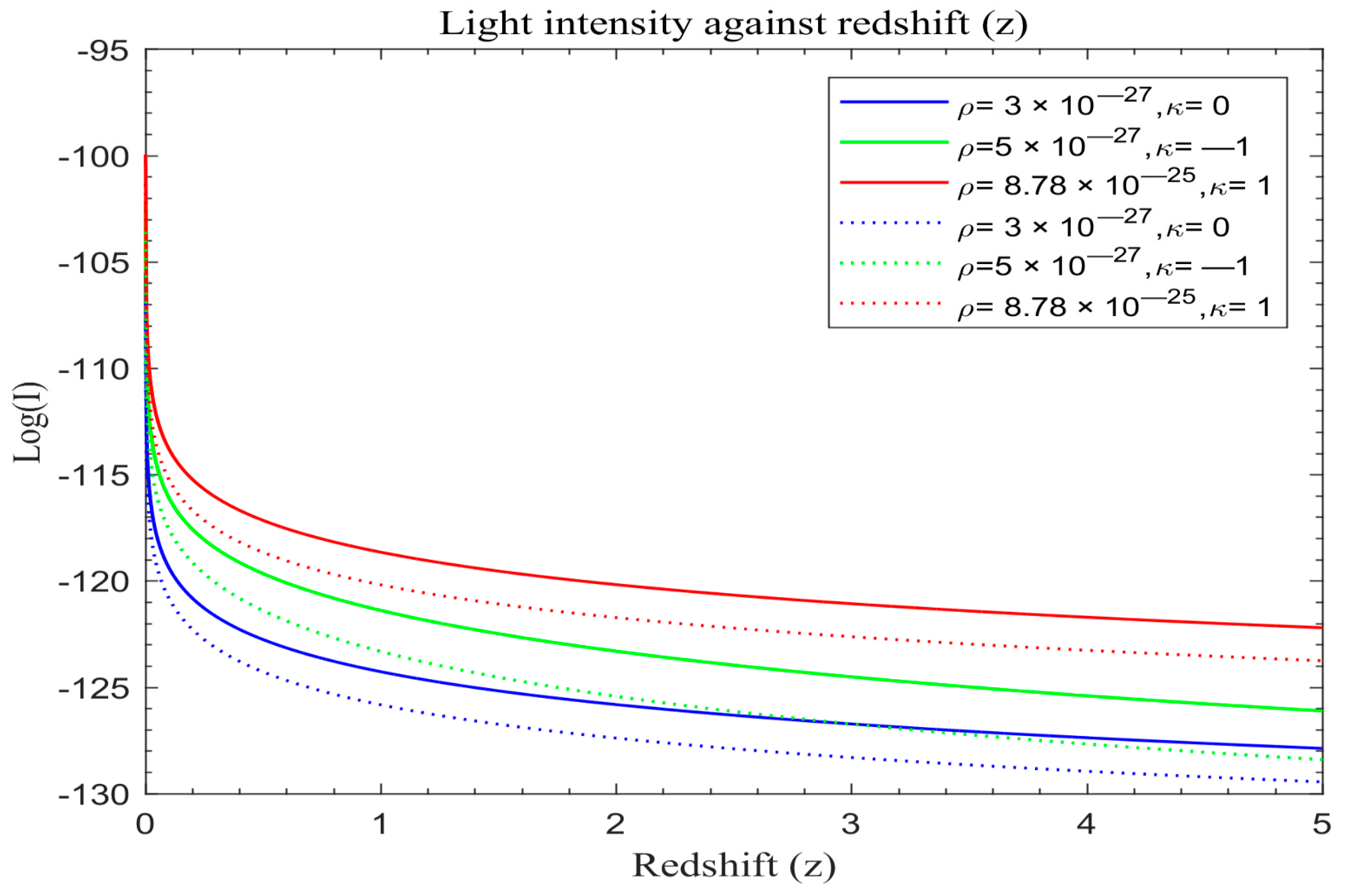
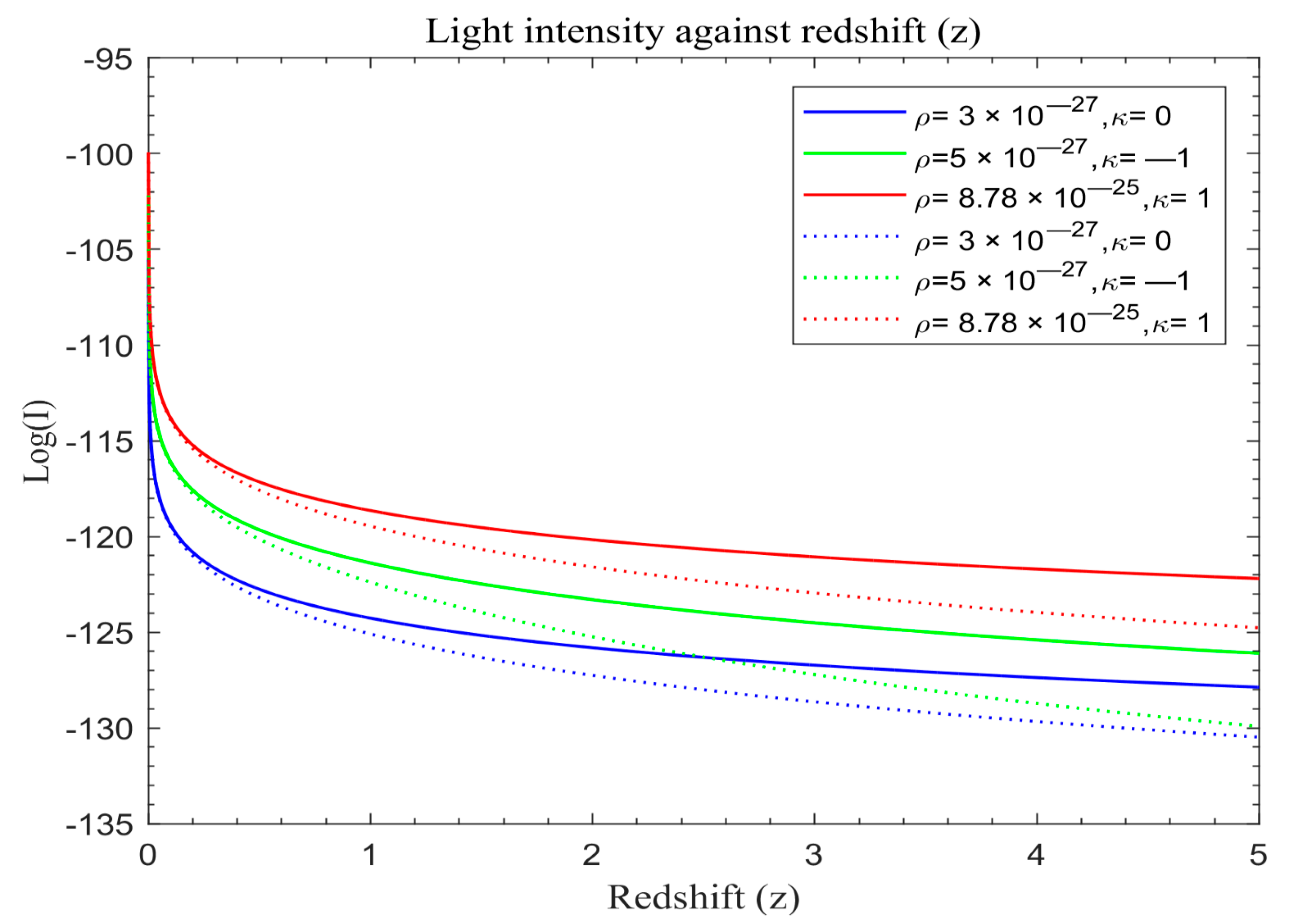
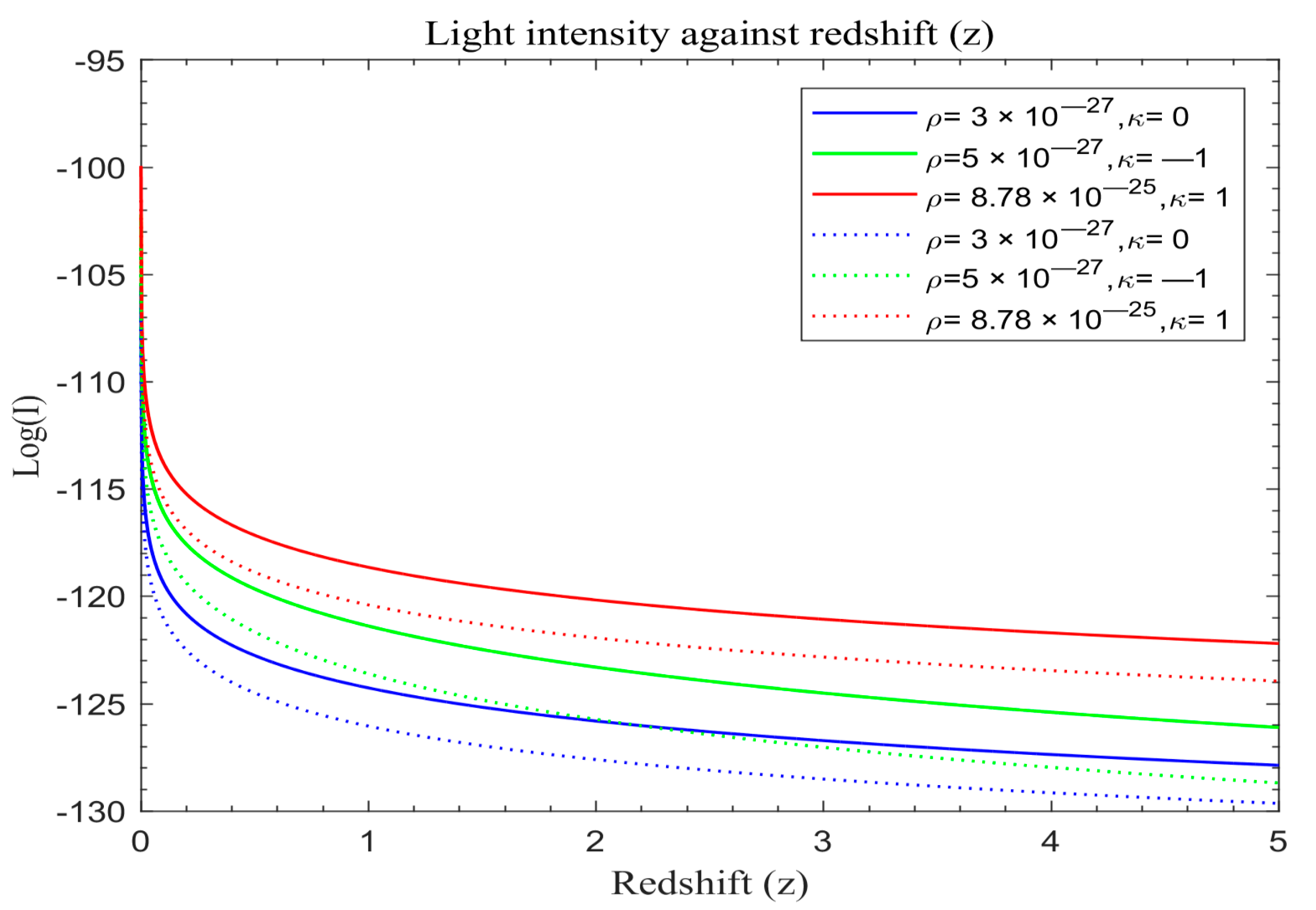
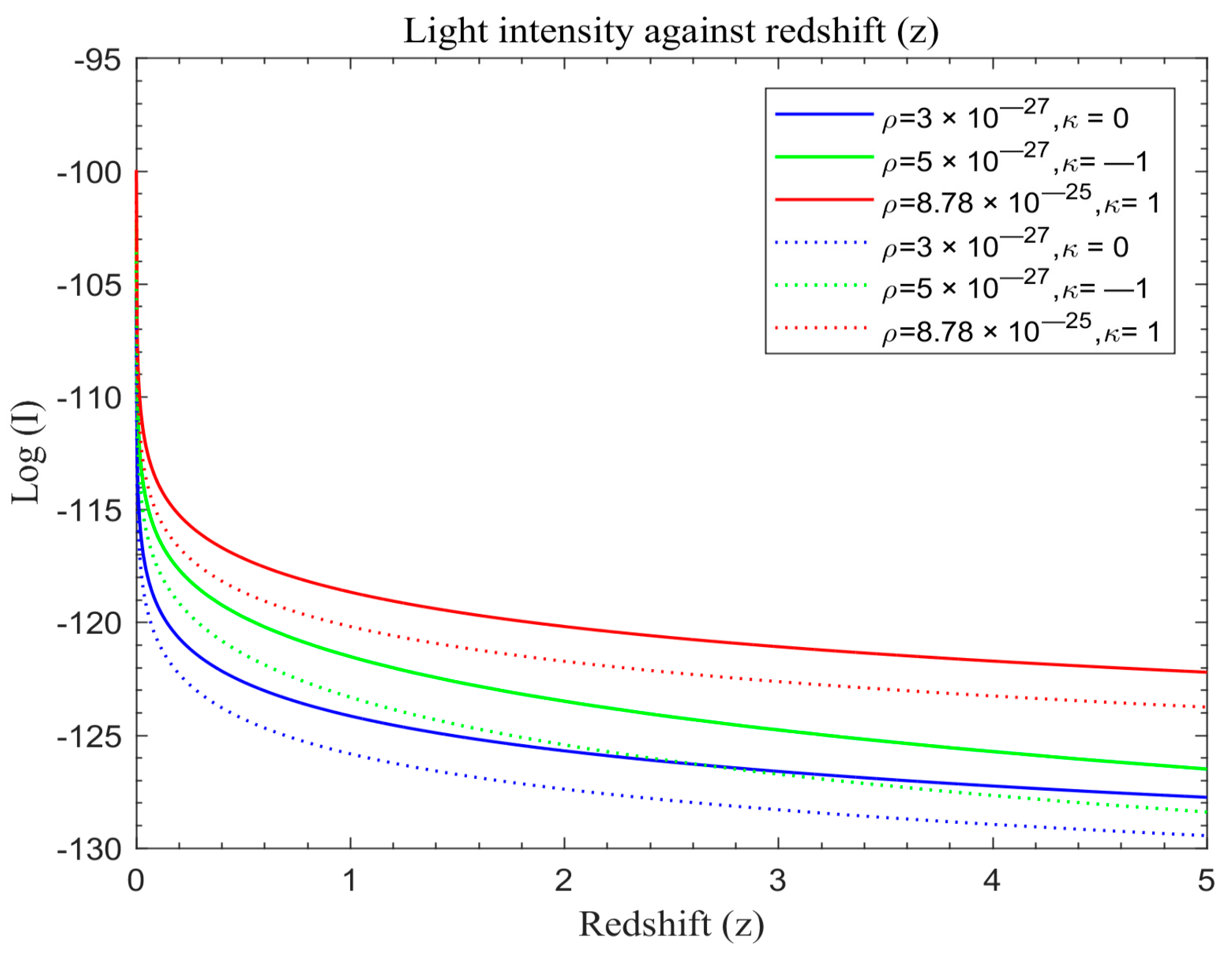
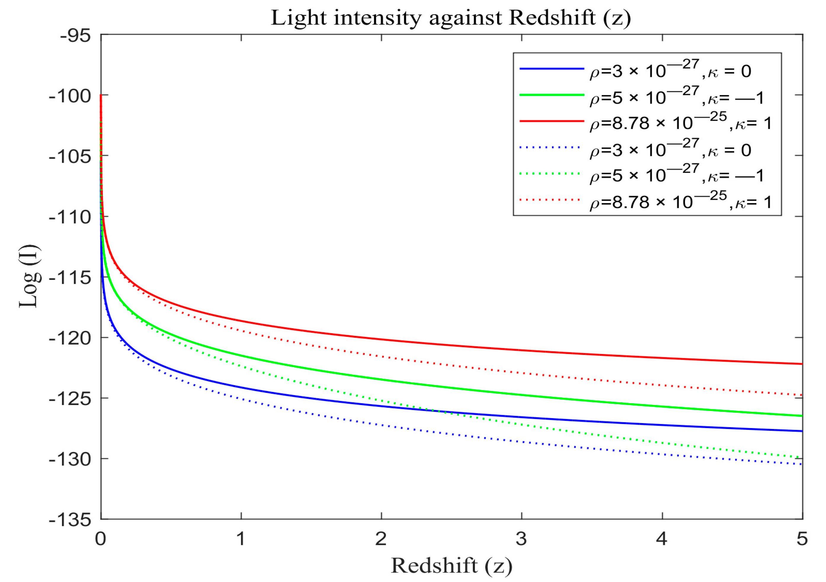
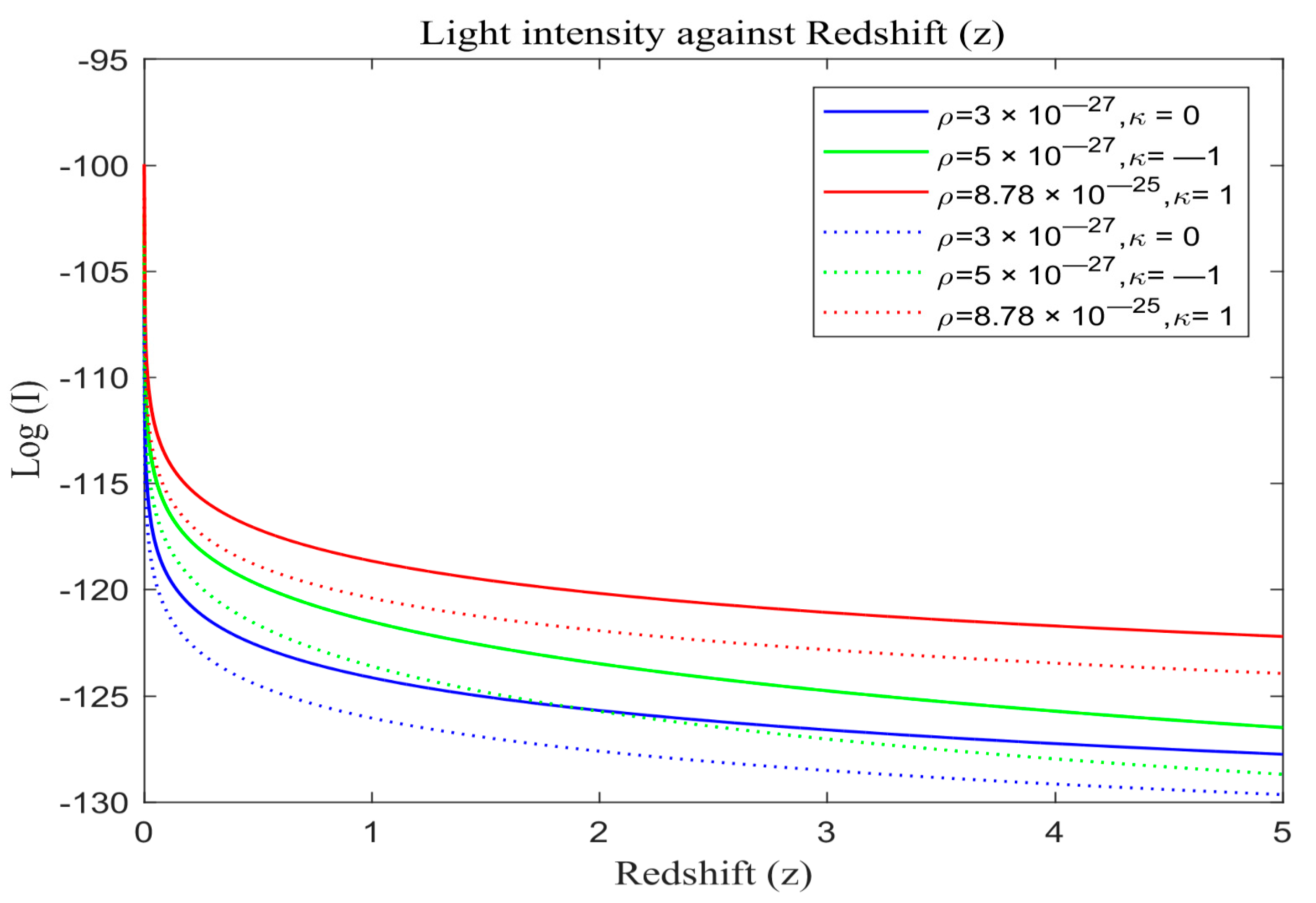
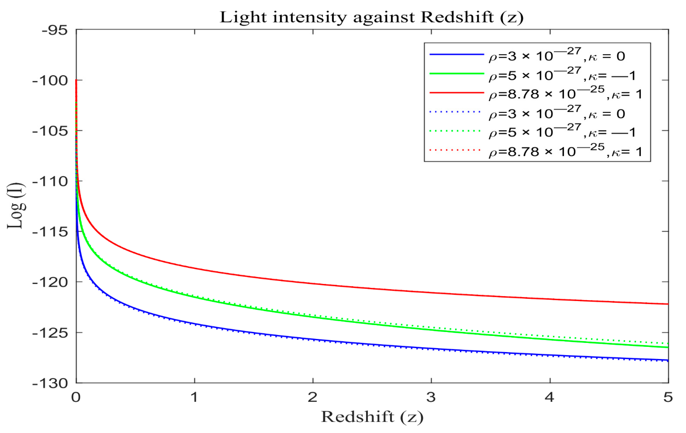
Figure 6 portray simulation outcomes for the evolution of light intensity for both the modified Friedmann model and the standard redshift model grounded in Equations (25) and (30) respectively. These visual representations offer a nuanced understanding of the intricate dynamics governing the evolution of cosmic structures under distinct cosmological paradigms. The standard redshift model displays the simulation results in solid lines while modified models are in dotted lines.
We also plot the standard redshift model with λ and the modified redshift model without λ on the same scale in order to assess the overall effects. The solid lines in
Figure 4,
Figure 5 and
Figure 6 portray the simulated results of light intensity with λ for the standard redshift model based on Equation (30), while the dotted lines represent the modified redshift model without λ based on Equation (30).
The light intensity of the standard redshift model with and without λ is also plotted on the same scale. The solid curves in
Figure 7 portray the simulated result of light intensity with λ for the standard redshift model based on Equation (30), while the dotted curves represent the light intensity of the standard redshift model without λ based on Equation (30).
4.2. Number Density–Redshift Graphs
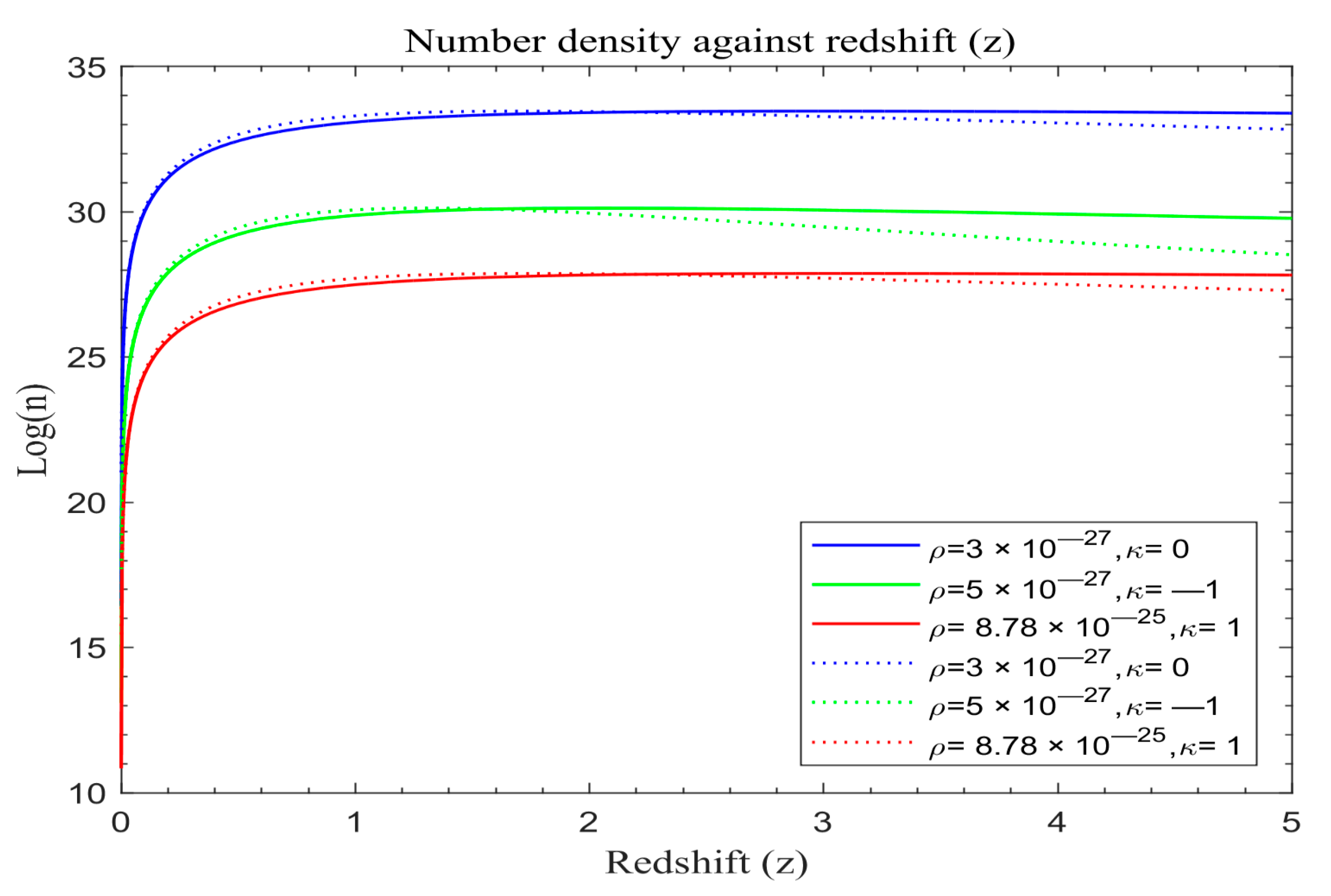
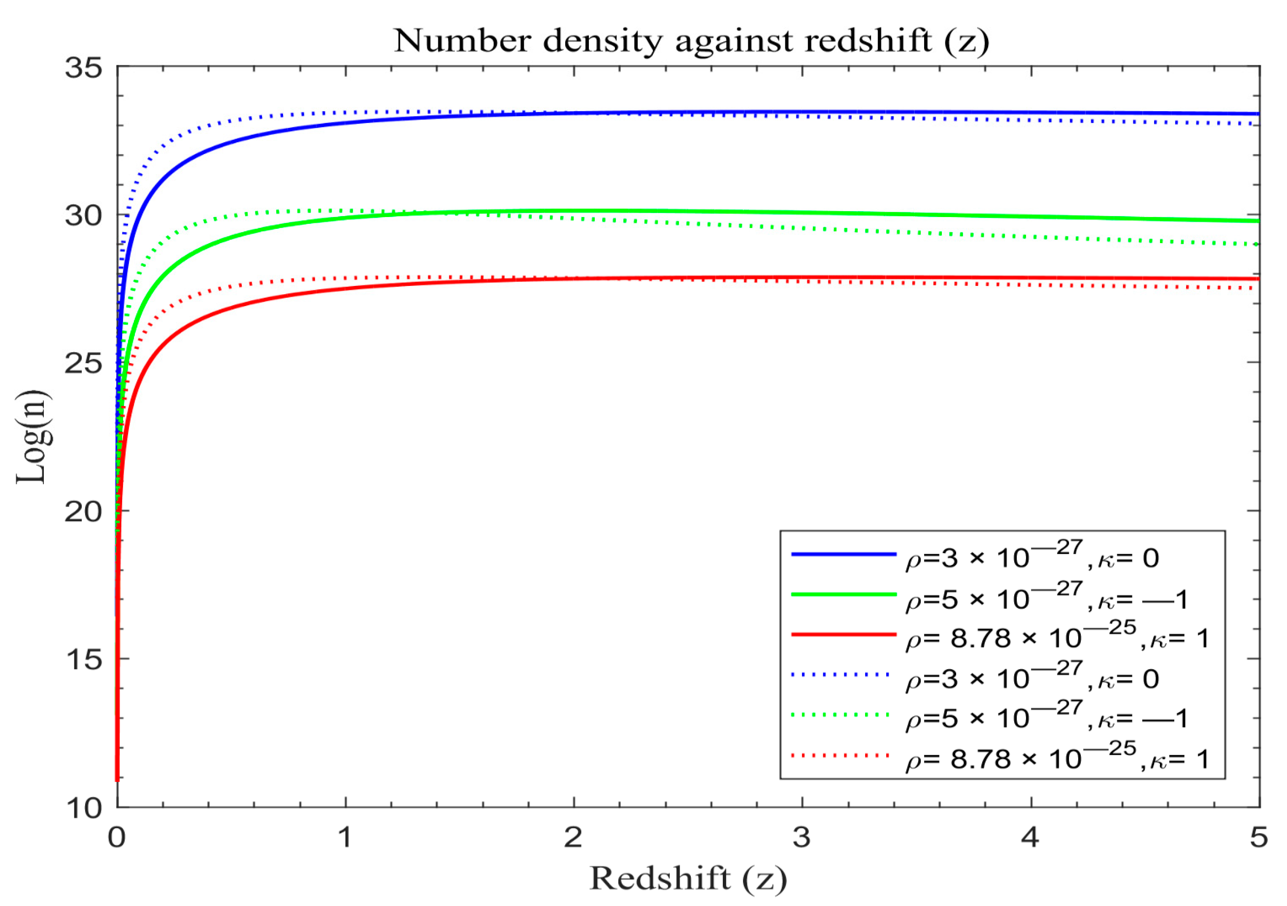
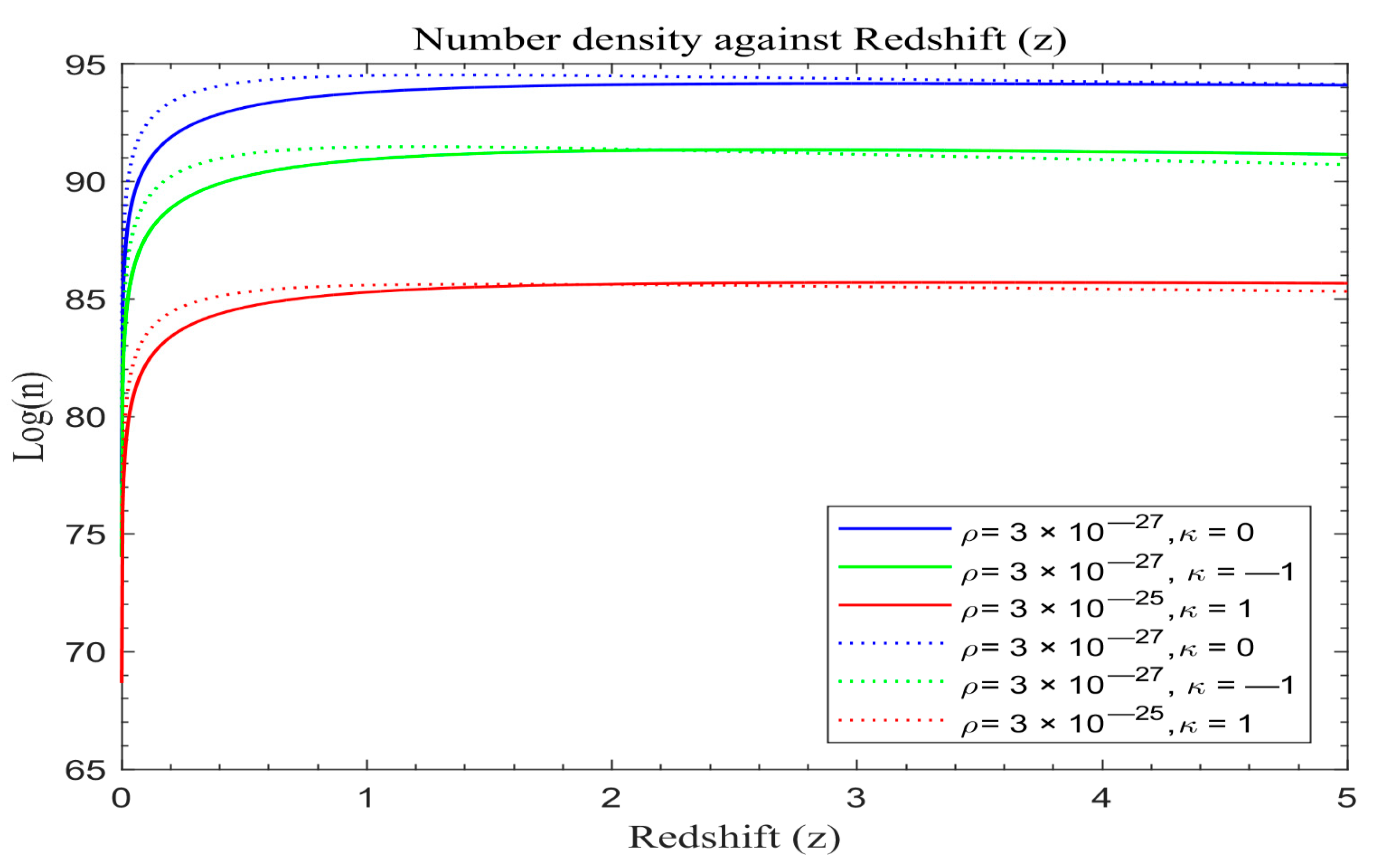
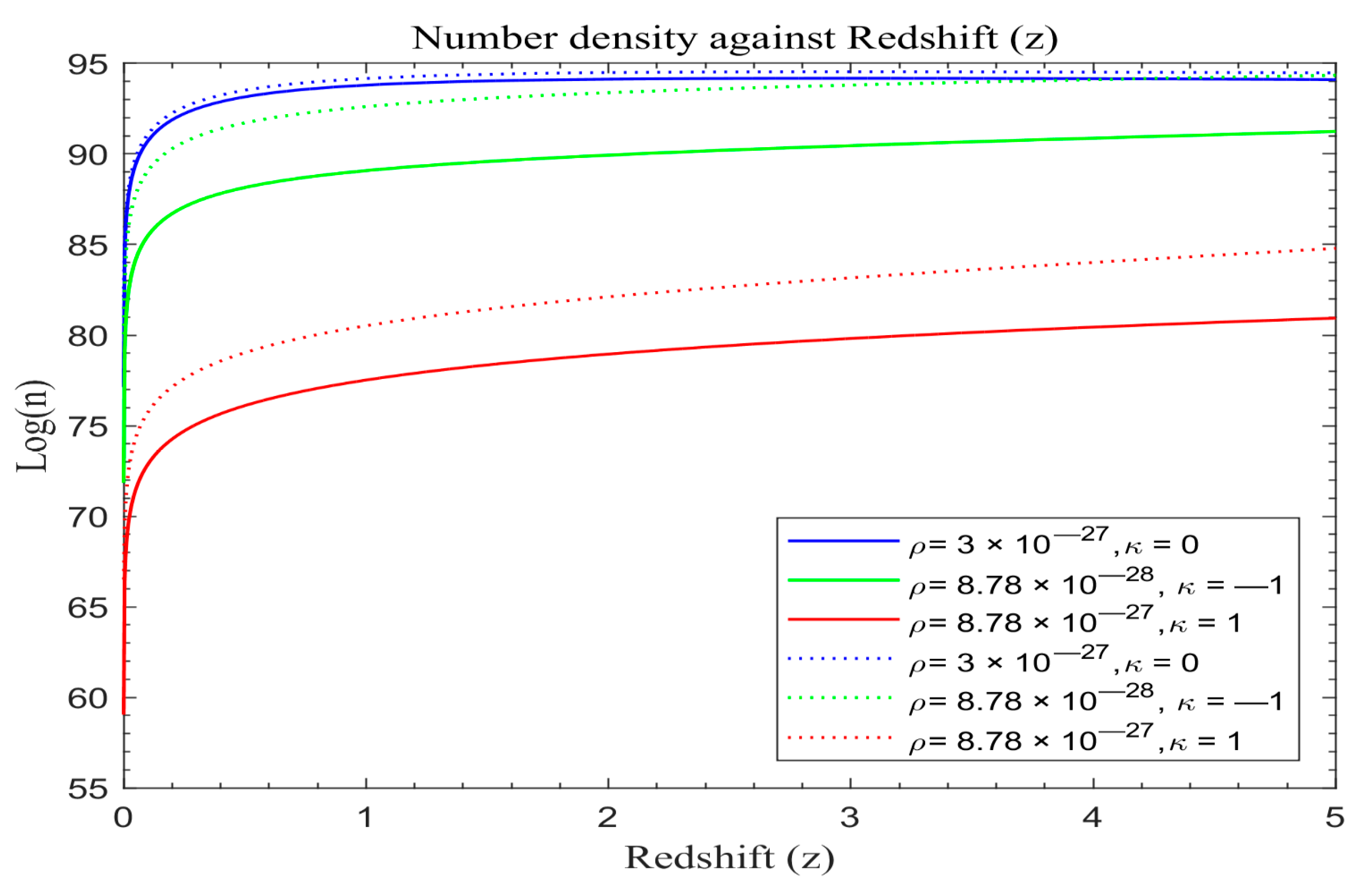
Figure 8,
Figure 9 and
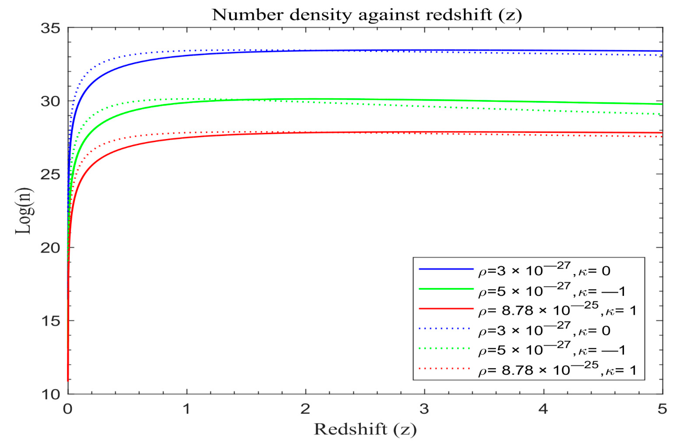
Figure 10 display the simulation results of number density of galaxy formation in the absence of cosmological constant for the modified redshift Friedmann model based on Equation (29).
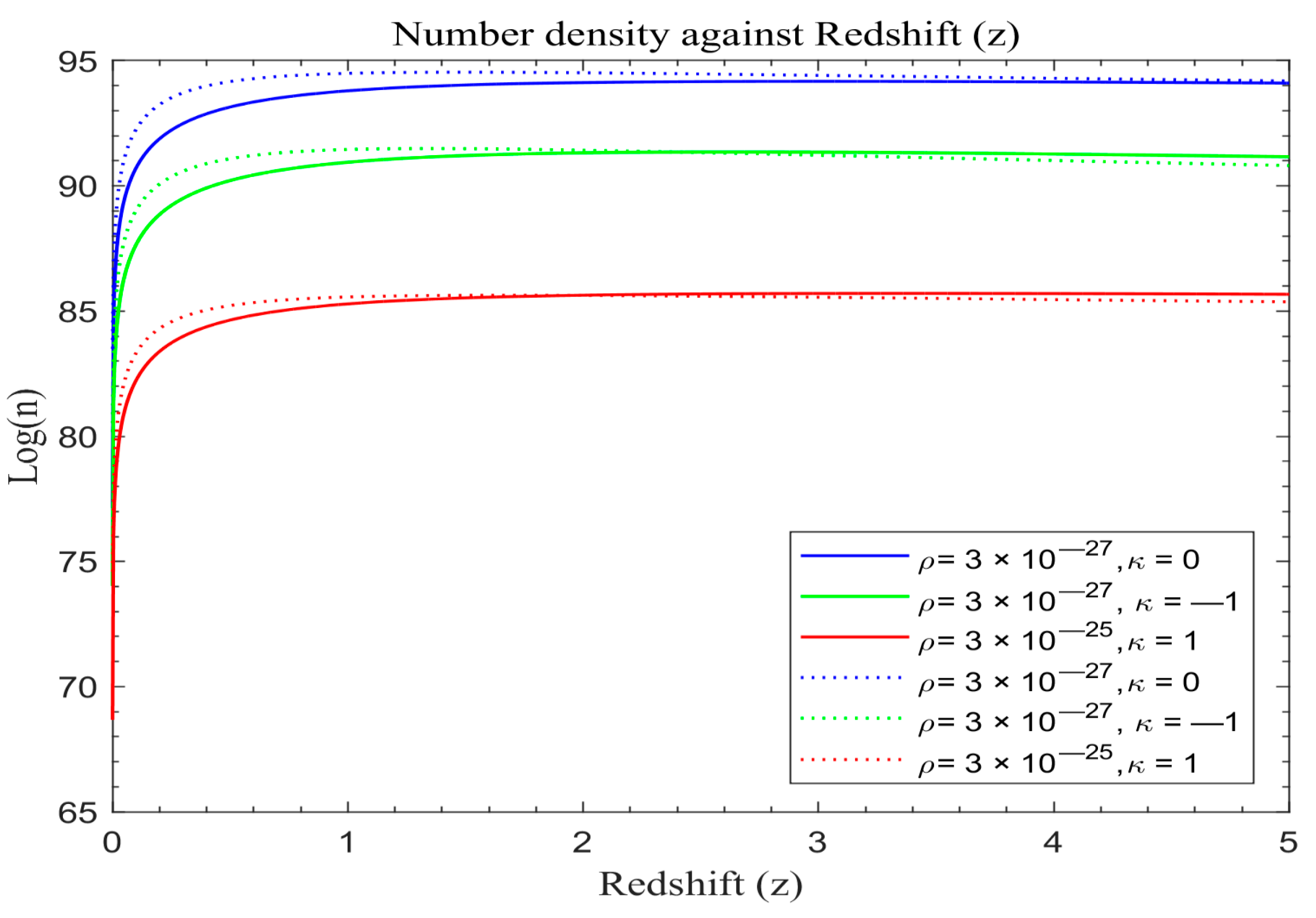
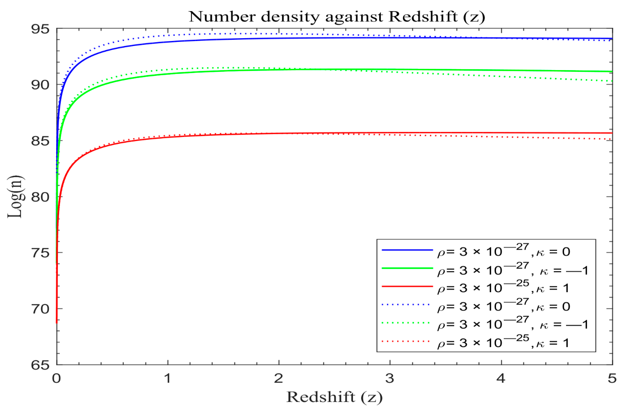
In order to assess the effect of the two models, let us plot the number density of galaxies of the standard redshift model with dark energy (λ) and the number density of galaxies of the modified redshift models without dark energy (λ = 0) on the same scale. The solid lines in
Figure 11,
Figure 12 and
Figure 13 portray the simulated result of the number density of galaxy formation with dark energy (λ) based on Equation (31), while the dotted lines represent the number density of galaxy formation for the modified redshift model in the absence of dark energy (λ = 0) based on Equation (28).
The number density of galaxies of the standard redshift model with dark energy is plotted together with the number density of galaxies of the standard redshift model with a vanishing dark energy (λ = 0) on the same scale, both graphs based on Equation (31). The solid curves in
Figure 14 portray the simulated result of the number density of galaxies with dark energy (λ) of the standard redshift model based on Equation (31), while the dotted curves represent the number density of galaxies of the standard redshift model with a vanishing λ based on Equation (31).
5. Discussion
5.1. Light Intensity of Galaxy Distribution
The attenuation of light intensity with redshift is visually depicted in
Figure 1,
Figure 2,
Figure 3,
Figure 4,
Figure 5,
Figure 6 and
Figure 7, covering various redshift ranges. In
Figure 1,
Figure 2 and
Figure 3, a distinct decrease in light intensity is evident across different universe models, transitioning from flat to open and then closed universes, regardless of the specific model applied. This attenuation is particularly pronounced in universes lacking dark energy and featuring modified redshift, suggesting a potential phenomenological link between cosmic expansion and dark matter. Furthermore, this phenomenon is influenced by the matter density and the curvature of the universe, as demonstrated by the similar attenuation rates between open and flat universes within the redshift range of z ≈ 2–2.4 before diverging.
Figure 4,
Figure 5,
Figure 6 and
Figure 7 demonstrate a similar trend of light attenuation as seen in
Figure 1,
Figure 2 and
Figure 3. Notably, in closed universes with dark energy, light intensity diminishes more rapidly compared to scenarios without dark energy, with this effect becoming more pronounced over time. Additionally, open universes demonstrate a higher attenuation rate compared to closed or flat universes, with the highest rate observed in closed universes, followed by open and flat universes, respectively. The influence of matter density and curvature remains consistent across these figures.
Analyzing the range of redshifts depicted in
Figure 1,
Figure 2 and
Figure 3, a discernible exponential attenuation pattern in the light intensity from galaxies is observed, regardless of the universe’s geometry. Intriguingly, modified light curves closely resemble standard redshift curves, indicating a level of universality in light intensity dynamics. However, a notable deviation is evident in the evolution of these intensity functions, especially in the modified model, diverging from the standard redshift model both in early epochs and in future projections. This temporal disparity aligns with theoretical propositions by [
48], who found that light intensity falls with redshift and is affected by dark energy, thereby bolstering the credibility of the modified model’s departure from conventional cosmic models. Results from [
54] regarding light from GRBs also confirmed these findings. Moreover, the modified redshift universe demonstrates a more rapid attenuation of light intensity with redshift compared to the standard redshift universe, as depicted in
Figure 1,
Figure 2 and
Figure 3. This divergence underscores the accelerated expansion posited by the modified model, contributing to the ongoing debate on cosmological models. The empirical validation of this accelerated expansion, supported by theoretical foundations laid out by [
48], emphasizes the significance of investigating the intricate relationship between theoretical frameworks and observational data.
The attenuation behavior of light is in line with classical expectations. As redshift increases, the ionizing sources decrease because structure formation slows down. Furthermore, space expansion and redshifting of photons leads to energy loss. Furthermore, an analysis of light pulse shapes originating from gamma rays, slow and fast neutron events, recorded separately using the Bollinger–Thomas single-photon method, showed a trend consistent with our results [
54].
5.2. Number Density of Galaxy Formation
The data represented in
Figure 8,
Figure 9,
Figure 10,
Figure 11,
Figure 12 and
Figure 13 reveal intriguing patterns wherein the modified redshift curves initially display accelerated growth, contrasting with the standard redshift model. However, both curves stabilize for a duration before diverging. Beyond a redshift value of z ≈ 1.6, the modified redshift curves start descending below those of the standard redshift. There is a phase of heightened galaxy formation within the redshift range of 0 < z < 0.4 across all universe models. Additionally, a significant proportion of galaxy formation appears to have occurred during 0 < z < 0.9, persisting, albeit at a slower pace, until around z ≈ 1.6. This observation is consistent with Marr’s findings [
55], who studied galaxy number counts in various bands (K, H, I, R, B, U) from the Durham Extragalactic Astronomy and Cosmology catalogue. In the model, bar graphs revealed a similar relationship between number density and redshift. Studies of massive compact galaxies from the BOSS spectroscopic dataset for the number density of galaxies against redshift in the range 0.2 < z < 0.6 further confirms our findings [
56].
Around z ≈ 0.9, the rate of galaxy formation in the modified redshift model decreases, unlike the relatively steady formation rate in the standard redshift model. This discrepancy suggests that the modified redshift model, indicative of a universe propelled by dark matter dynamics, fosters galaxy formation especially in the beginning. This finding agrees with [
57], who investigated the impact of dark matter on galaxy formation using N-body simulations. He found that baryonic matter gravitates towards great potential wells of dark matter halos where galaxies form initially rapidly before slowing down later. However, the rate of formation is intricately tied to both the matter density of the universe and its curvature characteristics.
Figure 11,
Figure 12,
Figure 13 and
Figure 14 depict a higher count of galaxies formed compared to
Figure 8,
Figure 9 and
Figure 10.
In examining the early stages of the universe, characterized by the initial burst of galaxy or star formation, a remarkable uniformity is observed among our models. The accelerating expansion of space, a key determinant in rendering any future accretion negligible, serves as a unifying factor at this emerging cosmic era. The indistinguishability of each model at early times lays the foundation for understanding the subsequent divergences in their evolutionary trajectories.
The historical divergence among our models becomes conspicuous in the late stages, primarily attributable to the onset of dark-matter-powered accelerated expansion. A notable consequence of this divergence is the elimination of the coincidence problem. Scenarios where λ equals zero equate to the era of matter growth that propels the cosmic accelerating force responsible for the late-time spatial acceleration. In the modified case, the departure from the standard redshift Friedmann model continues throughout all cosmic epochs, marking a significant achievement in this research.
Analyzing
Figure 8,
Figure 9,
Figure 10,
Figure 11,
Figure 12,
Figure 13 and
Figure 14, the number density of galaxy formation exhibits a rapid rise, culminating around z ≈ 1.6, followed by a gradual decline. The proposed model seems to undergo a phase of deceleration favoring galaxy formation in the early evolution of the universe, transitioning into an acceleration phase at later times. This critical transition from early deceleration to late-time acceleration is pivotal, as the decelerating phase is important for structure formation, while the slowdown of large-scale structure growth signifies the onset of dominant accelerating cosmic expansion. This observation is in line with recent work that suggests that dark matter provides the initial seed for star formation [
29,
57] further boost these findings.
As galaxies disperse due to the expanding universe, the processes of accretion and merging decelerate significantly, leading to a substantial reduction in the galaxy formation rate after peaking for future epochs. The total number density is predominantly dictated by contributions from the peak, stabilizing into a plateau around z ≈ 1.6 depending on the curvature characteristics and matter density. The role of the cosmological constant in shaping the structure formation in the universe appears less impactful in curtailing the late-time structure formation rate compared to the observed values in modified models, as evident in
Figure 11,
Figure 12 and
Figure 13.
Figure 8,
Figure 9,
Figure 10,
Figure 11,
Figure 12,
Figure 13 and
Figure 14 underscore that the universe, largely, has already produced the majority of its eventual structures, contributing only marginally to future developments.
The number density of galaxies increases with redshift with a remarkably constant value after peaking for the standard redshift model for future epochs, while that of the modified redshift model declines slowly thereafter peaking. The drop in galaxy number may be attributed to a fast increase in light intensity attenuation; producing strong repulsive forces at high redshifts (see light intensity curves in
Figure 1,
Figure 2,
Figure 3,
Figure 4,
Figure 5 and
Figure 6). For future epochs, gravitational forces may play a role in controlling the rate of decline, with the repulsive forces originating in light attenuation being negligible.
5.3. Comparing the Standard Redshift and the Modified Redshift Friedmann Cosmological Models
Within this section, our primary focus is on comparing the inherent properties of two cosmological models: the standard redshift Friedmann model and the modified redshift Friedmann model. As we explore cosmic time, a notable characteristic arises within the standard redshift model, where the universe’s expansion approaches a constant value asymptotically, outlining a distinct trajectory. In contrast, the modified redshift model exhibits a more gradual decline after reaching its peak. This subtle behavior results in a noticeable decrease in the number density conducive to galaxy formation, particularly in later epochs (refer to
Figure 8,
Figure 9 and
Figure 10). While different simulations of the modified Friedmann model show varied galaxy formations, both models demonstrate a consistent overall galaxy formation history. In future epochs, the modified universe transitions into an accelerating expansion era, with the growth rate of structures declining more slowly after peaking. Conversely, in the standard redshift model, we observe that galaxy growth approaches a constant value. This diverse formation pattern is linked to the expansion histories of universes with or without dark energy, as represented by the standard redshift and modified redshift models. Graphical representations illustrate a notable disparity between the trajectories outlined by the standard redshift and modified redshift models (see
Figure 11,
Figure 12 and
Figure 13. This clear distinction serves as empirical evidence of the influence of dark matter driving accelerated expansion [
29]. Despite this gap, both cosmologies share a commonality in the culmination of galaxy formation in the early universe. It is essential to recognize that as time progresses, the universe undergoes a transformative shift, with cosmic acceleration playing a crucial role. Concurrently, it may be that the influence of dark matter suppresses the overarching structure formation, shaping the fate of galaxies as the universe evolves.
In a nutshell, while our model statistically aligns with the standard redshift Friedmann paradigm during the early stages of the universe’s evolution, a distinctive trajectory emerges at later stages as highlighted in
Figure 8,
Figure 9,
Figure 10,
Figure 11,
Figure 12 and
Figure 13.
5.4. Transition from Decelerating to Accelerating Expanding Universe
This section concentrates on identifying the suppression point within the structure amplitude, a key aspect of our simulation concerning the number density of galaxies. This investigation aids in predicting the transition point between deceleration and acceleration in our modified cosmological model.
A comprehensive analysis of
Figure 8,
Figure 9,
Figure 10,
Figure 11,
Figure 12 and
Figure 13 reveals a significant trend in galaxy formation. In the early stages of the universe, galaxies form rapidly, experiencing a burst of stellar or galactic activity between redshift 0 < z < 0.4. This rate peaks around z ≈ 0.9 before slowing down significantly, maintaining a relatively constant level of galaxy formation until z ≈ 1.6 where this process starts to decline, as evident in
Figure 8,
Figure 9,
Figure 10,
Figure 11,
Figure 12 and
Figure 13. This result agrees with [
58], who found that the onset of cosmic acceleration was consistent with observations of distant spiral galaxies exhibiting a gradual decline or near constancy in galaxy formation over time.
The universe may have undergone a shift from a phase of decelerating expansion after its climax to accelerated expansion. It has been found that the universe undergoes a series of redshift transitions, as demonstrated by [
2], who noted the universe’s mass-energy content transitions from matter domination to an acceleration-dominated state. The persistence of accelerated expansion requires overcoming gravitational attraction forces exerted by the cosmological fluid, primarily composed of ordinary matter.
In our model framework, the transition from deceleration to acceleration expansion occurs at a specific redshift. Our findings suggest that a transition from matter domination to acceleration expansion is feasible only if the energy effects driving the universe into acceleration begin in an epoch z ≈ 0.9. This value is in fair agreement with the best-fit value of 0.732 < z < 0.966 [
59,
60]. However, any observed disparities with other models could stem from variations in models or underlying assumptions used. However, pinpointing the accurate redshift transition point requires calibrating model parameters against cosmological data. This approach was suggested by [
61], who predicted a plausible temporal transition from a matter-dominated universe to a dark-energy-dominated universe, emphasizing the importance of fitting model parameters to observational data for precise and reliable cosmological predictions.
5.5. Meaning of Our Results
The investigation into the evolution and distribution of galaxy number density has yielded intriguing results, with various modified models consistently predicting an accelerating expanding universe. Despite subtle variations in underlying mechanisms, these models converge on the same analytical outcome concerning the magnitude of observed structure formation compared to the widely accepted standard redshift Friedmann model. Indeed,
Figure 8,
Figure 9,
Figure 10,
Figure 11,
Figure 12 and
Figure 13 illustrate trajectories of different structures formed by standard redshift and modified redshift models, indicating a notable disparity and suggesting the pivotal role of dark matter in late-time acceleration.
These figures emphasize the essence of our findings, revealing alignment between the modified redshift relation and a positive cosmological constant within a standard redshift model. This alignment implies an excess of dark energy introduced by the cosmological constant, leading to a gradual flattening of the structure formation amplitude profile. Surprisingly, our results challenge the conventional wisdom, suggesting that a cosmological constant or other form of dark energy, characterized by peculiar negative pressure, may not be necessary to explain the observed accelerating expansion of the universe. The notion of suppressing structure amplitudes emerges as a pertinent condition for the viability of our dark-matter-dominated cosmological model.
Despite differences in structural growth rates, the impact of accelerated expansion due to a modified redshift becomes significant only after the majority of structures have formed, resulting in a decrease in the total number density of galaxies. Remarkably, the modified redshift model successfully accounts for most observational signatures of cosmic acceleration.
Intriguingly, simulations devoid of dark energy predict a crossover in the cosmic galaxy formation rate, transitioning from deceleration to acceleration. These findings underscore the complexity of cosmic dynamics and highlight the intricate interplay between various factors influencing the evolution of our expansive universe.
6. Summary and Conclusions
The present astronomical inquiry stands as a diligent effort to scrutinize the fundamental principle of cosmology, specifically addressing the homogeneity and isotropy assumptions inherent in the Friedmann model. Extensive research has already been dedicated to testing spatial isotropy through a spectrum of techniques and probes. Nevertheless, the homogeneity hypothesis presents a formidable challenge, prompting a focused investigation [
18,
19]. The study is focused on three fundamental astronomical quantities: number density, light intensity, and redshift. It explores the interrelationship between these quantities in both the standard redshift Friedmann model and its modified form proposed within the research. The study extends the groundwork laid by prior research on the Friedmann model [
48]. The driving force arises from a modification of the conventional redshift, providing a fresh perspective on the Friedmann equations.
This reinterpretation is grounded in a phenomenologically modified redshift model, deliberately devoid of dark energy through the elimination of the cosmological constant.
The modified redshift, as introduced in this study, serves as a novel instrument for characterizing the distribution of luminous matter within the cosmic framework. Emphasizing the Friedmann model, the investigation is particularly attuned to the growth rate of cosmic structures. This parameter emerges as a discerning factor, keen to differentiate between the general-relativity-backed standard redshift Friedmann model and the alternative scenarios rooted in its modified form. The overall goal is to establish a framework for discerning between competing cosmological models.
Distinct phenomenologically modified redshift models, namely parametric [
40] and non-parametric [
42] models, are systematically explored within the context of a matter-dominated Friedmann universe. The analytical prowess of this study is demonstrated through the rigorous solution of relativistic dynamic Friedmann equations as given in Equations (25) and (28)–(31). Compared to earlier research [
48], Equations (25), (28) and (29) are presented in a more generalized form, describing the relationship between light intensity and redshift, as well as the relationship between number density and redshift. These solutions, in turn, shed light on the light intensity and number density of galaxies, describing their evolution as functions of the modified redshift as seen in
Figure 1,
Figure 2,
Figure 3,
Figure 4,
Figure 5 and
Figure 6 and
Figure 8,
Figure 9,
Figure 10,
Figure 11,
Figure 12 and
Figure 13, respectively.
The early consideration of dark energy within the framework is a methodological choice, enabling subsequent analyses to nullify its impact. This is achieved by setting the cosmological constant to zero in Equations (30) and (31) for modified redshift dark-matter-powered phenomenological models.
Simulations are then meticulously executed utilizing MATLAB applications. The simulation spans the redshift range from 0 to 5, revealing intriguing dynamics. The simulation reveals a unique pattern of galaxy formation, marked by a significant burst between redshifts 0 < z < 0.4. This burst then transitions into a gradual rise up to z ≈ 0.9, after which galaxy formation proceeds slowly at a nearly constant rate until z ≈ 1.6. Thereafter, a decline in structure formation becomes possible, as illustrated in
Figure 8,
Figure 9,
Figure 10,
Figure 11,
Figure 12 and
Figure 13. Furthermore, simulations without dark energy unveil a phase crossover point in the cosmic galaxy formation rate, marking the transition from deceleration to accelerating expansion at redshifts around z ≈ 1.6, as seen from
Figure 8,
Figure 9,
Figure 10,
Figure 11,
Figure 12 and
Figure 13. Our number density relation is in excellent agreement with other works [
55,
58]. Simulations of light intensity functions reveal light attenuation with redshift evident in
Figure 1,
Figure 2,
Figure 3,
Figure 4,
Figure 5,
Figure 6 and
Figure 7, which is in fair agreement with the GRB results and light pulse distribution shapes [
54]. The modified redshift universe shows that light intensity distribution attenuates more rapidly with the standard redshift as compared to the modified redshift model (
Figure 1,
Figure 2,
Figure 3,
Figure 4,
Figure 5 and
Figure 6).
A critical observation emerges concerning the differential impact of the cosmological constant on structure formation. The study posits that the cosmological constant within the standard redshift model exhibits a less pronounced effect on late-time structure formation growth compared to the modified model in agreement with observational evidence [
62]. This nuanced disparity underscores the prowess of the modified model. The expansion of the universe beyond z > 0.9 is attributed to dark-matter-powered cosmic acceleration rather than the effect of the cosmological constant (
Figure 8,
Figure 9,
Figure 10,
Figure 11,
Figure 12 and
Figure 13). Despite differences in the rate of structural growth, the impact of accelerated expansion becomes significant only after the majority of structures have been formed.
The study concludes with a resolute stance against the necessity of introducing the cosmological constant into the modified model. The latter, characterized by a positive cosmological constant in the context of the standard redshift model, eliminates the need for a cosmological constant, thereby avoiding excessive dark energy and eliminating the necessity for fine tuning at an implausibly small degree. The relentless acceleration of the universe in its later stages is proposed as a firmly established and almost model-independent theoretical certainty, unaffected by ongoing debates about the nature of the cosmological constant.
The proposed modified model’s ability to accurately capture most of the discernible signatures of cosmic acceleration underscores its novelty. Therefore, the expansion evolution of the universe might be a result of the imbalance of gravitational forces and dark matter. The call for future inquiry echoes a commitment to testing with future accurate cosmological data. This paper, rooted in the analysis and scrutiny of cosmological models, contributes to the ongoing debate on the dynamic evolution of our universe.

 ,
, 


