
Generating Stellar Spectra Using Neural Networks

Department of Chemistry and Physics, Saint Mary’s College, Notre Dame, IN 46556, USA
Astronomy 2024, 3(1), 1-13; https://doi.org/10.3390/astronomy3010001
Submission received: 13 November 2023
/
Revised: 23 January 2024
/
Accepted: 24 January 2024
/
Published: 30 January 2024
Abstract
:A new generative technique is presented in this paper that uses Deep Learning to reconstruct stellar spectra based on a set of stellar parameters. Two different Neural Networks were trained allowing the generation of new spectra. First, an autoencoder is trained on a set of BAFGK synthetic data calculated using ATLAS9 model atmospheres and SYNSPEC radiative transfer code. These spectra are calculated in the wavelength range of Gaia RVS between 8400 and 8800 Å. Second, we trained a Fully Dense Neural Network to relate the stellar parameters to the Latent Space of the autoencoder. Finally, we linked the Fully Dense Neural Network to the decoder part of the autoencoder and we built a model that uses as input any combination of , , , , and and output a normalized spectrum. The generated spectra are shown to represent all the line profiles and flux values as the ones calculated using the classical radiative transfer code. The accuracy of our technique is tested using a stellar parameter determination procedure and the results show that the generated spectra have the same characteristics as the synthetic ones.
1. Introduction
Most of the stellar spectroscopy analysis techniques require synthetic data in order to be tested and constrained [1,2,3,4,5]. Astronomers have used radiative transfer codes to simulate the spectra of specific stars, planets, galaxies, and other astronomical objects. Synthetic stellar spectroscopy relies on a limited combination of model atmospheres and radiative transfer codes. It is worth mentioning the MARCS/Turbospectrcum models [6,7] that are mainly used for giant and dwarf stars. MOOG code [8] is able to perform a variety of LTE line analysis and spectrum synthesis tasks. ATLAS/SYNTHE/WIDTH [9,10] is used for spectral synthesis and the derivation of chemical abundances from equivalent widths of spectral lines. SME [11] is capable of deriving stellar parameters and chemical composition for a broad range of stars, including cool dwarfs and giants. SYNSPEC [12,13,14], used in this work, can synthesize spectra of stars with effective temperatures () ≥ 4000 K. Finally, PHOENIX models [15] are well suited for stars having ≤ 12,000 K.
When users do not have direct access to these codes and wrappers, they use data from available online databases. These databases are usually calculated with large steps in and surface gravity, , leading to large uncertainties on the derived stellar parameters once compared with true observations. Examples of these databases are POLLUX [16] which contains spectra of stars varying in , , and metallicity (). TLUSTY is a Non-LTE Line-blanketed model atmosphere of O-type stars [17] with ≥ 27,500 K. For cooler stars, the AMBRE database contains high-resolution FGKM synthetic spectra [18].
In this work, we suggest a new technique based on Artificial Neural Networks (ANN), which learn from the relation between stellar parameters and the flux of synthetic data and then allow the user to calculate a synthetic spectrum by providing the ANN a combination of , , , projected equatorial rotational velocity (), microturbulence velocity (), and resolution. The advantage of such a technique is that it only requires that Python (version 3.9.7) is installed and does not need to have any compiler such as Fortran or C++ nor a radiative transfer code. Ultimately, one would use this technique to train an ANN using well-known observed spectra. The spectra should have a large range of wavelength, stellar parameters, and individual chemical abundances. This can only be achieved by combining the data from different surveys to increase the wavelength range of the spectra. Being able to reproduce stellar spectra without the use of model atmospheres and radiative transfer code will make spectral synthesis homogeneous across the HR-Diagram. It will also allow the comparison of results among different studies, as we will not be faced with the classical issue of using different physics in different types of models (e.g., MARCS vs. ATLAS or Turbospectrcum vs. SYNSPEC).
For the sake of the proof of concept, this paper will detail the technique when applied to a small wavelength range. We have chosen the range of Gaia Radial Velocity Spectrometer (RVS, [19]) based on the fact that it has more than one million mean spectra [20] and that it contains a small wavelength range ( between 8400 and 8800 Å), making the calculation of the training database less time-consuming. The RVS will provide spectra in the CaII IR triplet region combined with weak lines of Si I, Ti I, Fe I, among others. Weak lines of N I, S I, and Si I and strong Paschen hydrogen lines can be found in A and F stars. For stars hotter than A0, spectra may contain lines of N I, Al II, Ne I, Fe II, and He I [21]. RVS spectra contain valuable information about the stellar parameters, as will be discussed in this paper.
Section 2 will explain the construction of the synthetic database and the Neural Networks (NNs) used in this work. Section 3 will show the newly generated spectra that will be tested against a stellar parameters derivation technique. Finally, the discussion and conclusions will be presented in Section 4.
2. Materials and Methods
The technique of generating synthetic spectra requires several steps. The first one is to calculate the database of synthetic data, the second step requires building autoencoders in order to reduce the dimension of the original flux to fewer data points that are saved in a Latent Space, and finally, the fundamental parameters are related to the Latent Space through a fully connected NN. Conceptually, we will be developing a model that takes as an input the stellar parameters and generates as an output a synthetic spectrum. An extra step was performed in Section 3 for deriving the stellar parameters of the generated dataset. The purpose of this step is to check the reliability and accuracy of the generated data.
2.1. Training Database
The details of calculating a training database are fully explained in [3]. In summary, Line-blanketed model atmospheres were calculated for the purpose of this work using ATLAS9 (Kurucz, 1992). These are LTE plane parallel models that assume hydrostatic and radiative equilibrium. We have used the Opacity Distribution Function (ODF) of [22]. Using Smalley’s prescriptions [23], we have included convection in the atmospheres of stars cooler than 8500 K. We have treated convection using the mixing length theory. A mixing length parameter of 0.5 was used for 7000 K ≤ ≤ 8500 K, and 1.25 for ≤ 7000 K. The synthetic spectra grid was computed using SYNSPEC [12] according to the parameters described in Table 1. Metallicity was scaled, with respect to the Grevesse & Sauval solar value [24], from −1.5 dex up to +1.5 dex. The metallicity is calculated as the abundance of elements heavier than Helium. The change in metallicity consists of a change in the abundance of all metals with the same scaling factor. The synthetic spectra were computed from 8400 Å up to 8800 Å with a wavelength step of 0.10 Å. This range is chosen to include the RVS range. The Resolution, (), also varies around the nominal RVS one, which is around 11,500 [19]. As explained in [25], the RVS spectra contain lines with information on the chemical abundance of many metals ( Mg, Si, Ca, Ti, Cr, Fe, Ni, and Zr, among others) that have different ionization stages and are sensitive to the stellar parameters. We have used the line list of [3].
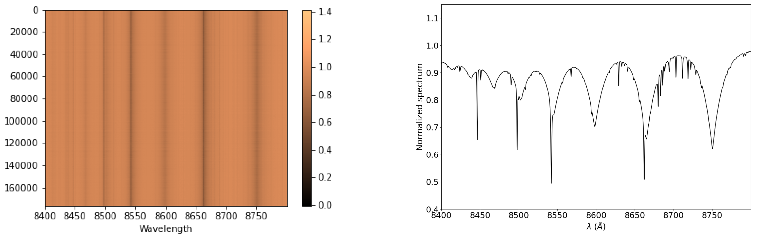
We ended up with a database of 205,000 synthetic spectra with , , , , , and resolution chosen randomly from Table 1. The left side of Figure 1 shows a color map of a sub-sample of the database. The absorption lines of the calcium triplet ( = 8498, 8542, 8662 Å) are easily detected in the figure. The right side of Figure 1 displays an example of a synthetic spectrum having a , , , , , and resolution of 9950 K, 3.50 dex, 2 km/s, 0.5 dex, 1.3 km/s, and 11,500, respectively.
2.2. Autoencoder
Autoencoders, usually used in denoising techniques [26,27], are a type of ANN used in unsupervised machine learning and deep learning. They are primarily used for dimensionality reduction and data compression. Autoencoders usually replace Principal Component Analysis (PCA) because of their non-linear properties. Autoencoders consist of two algorithms, an encoder and a decoder. They usually work by learning a compact representation of the input data within a lower-dimensional space (Latent Space) and then reconstructing the original data from this representation.
All the calculations that are presented in this paper were carried out using the Machine Learning platform TensorFlow1 (version 2.9.1) with the Keras2 (version 2.9.0) interface and were written in Python. We used a computer that has 52-2.1 GHz cores, Nvidia RTX A6000 48 GB graphic card, 256 GB of RAM, and 12 TB of data storage.
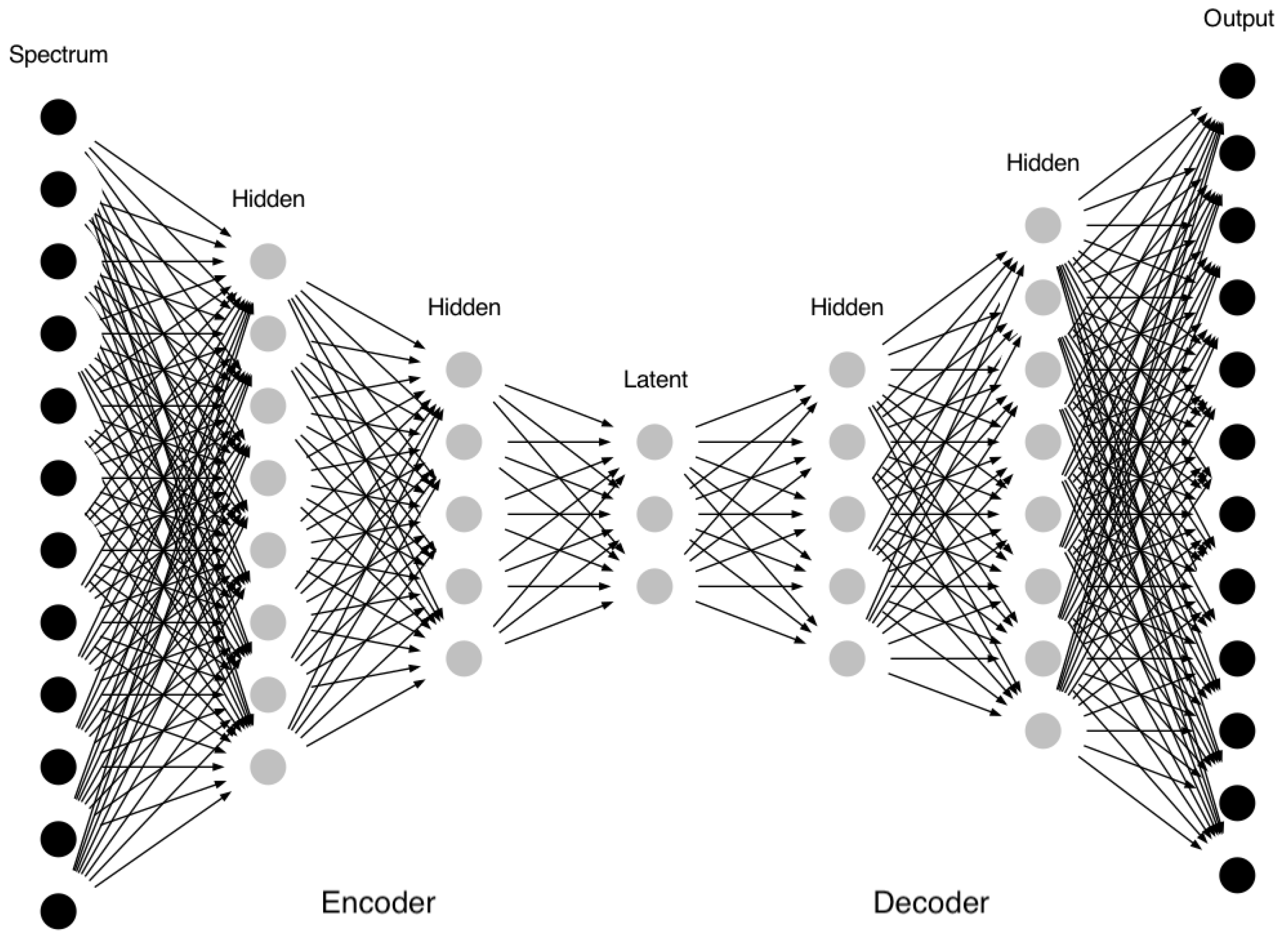
The architecture of the autoencoder is shown in Figure 2 in which the initial spectrum is introduced having 4000 data points ( between 8400 and 8800 Å with a step of 0.1 Å). It is then reduced to 10 parameters inside a Latent Space by passing it through a series of hidden layers of different sizes. There is no straightforward rule that relates the size of the Latent Space as a function of the input. However, we were inspired by the work of [28] and [1,3] in which the authors were able to represent a larger spectral range with only 12 points using PCA. We have used a Latent Space with a dimension of 10 for our spectra. All architectures used in this work as well as the choice of the hyperparameters were constrained using the technique introduced in [2]. The optimal parameters are the results of a minimization procedure of the loss function (see [2] for more details).
The steps that transform the spectrum from its original 4000 data points to 10 from the encoder part of the autoencoder. A symmetrical counterpart, a decoder, transforms the 10 data points to their original values of 4000. The characteristics and parameters used in this autoencoder are presented in Table 2.
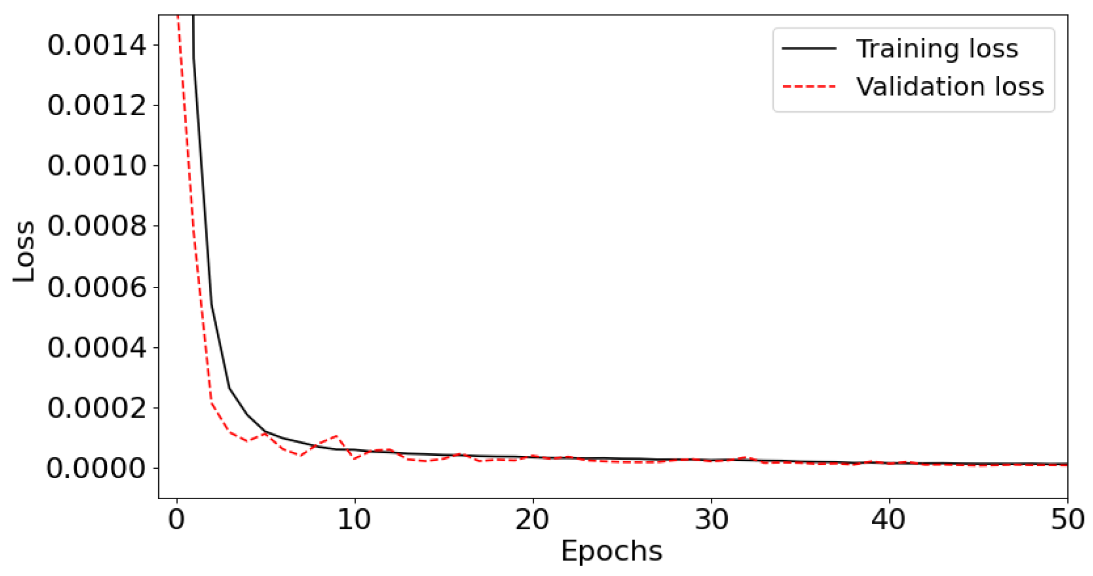
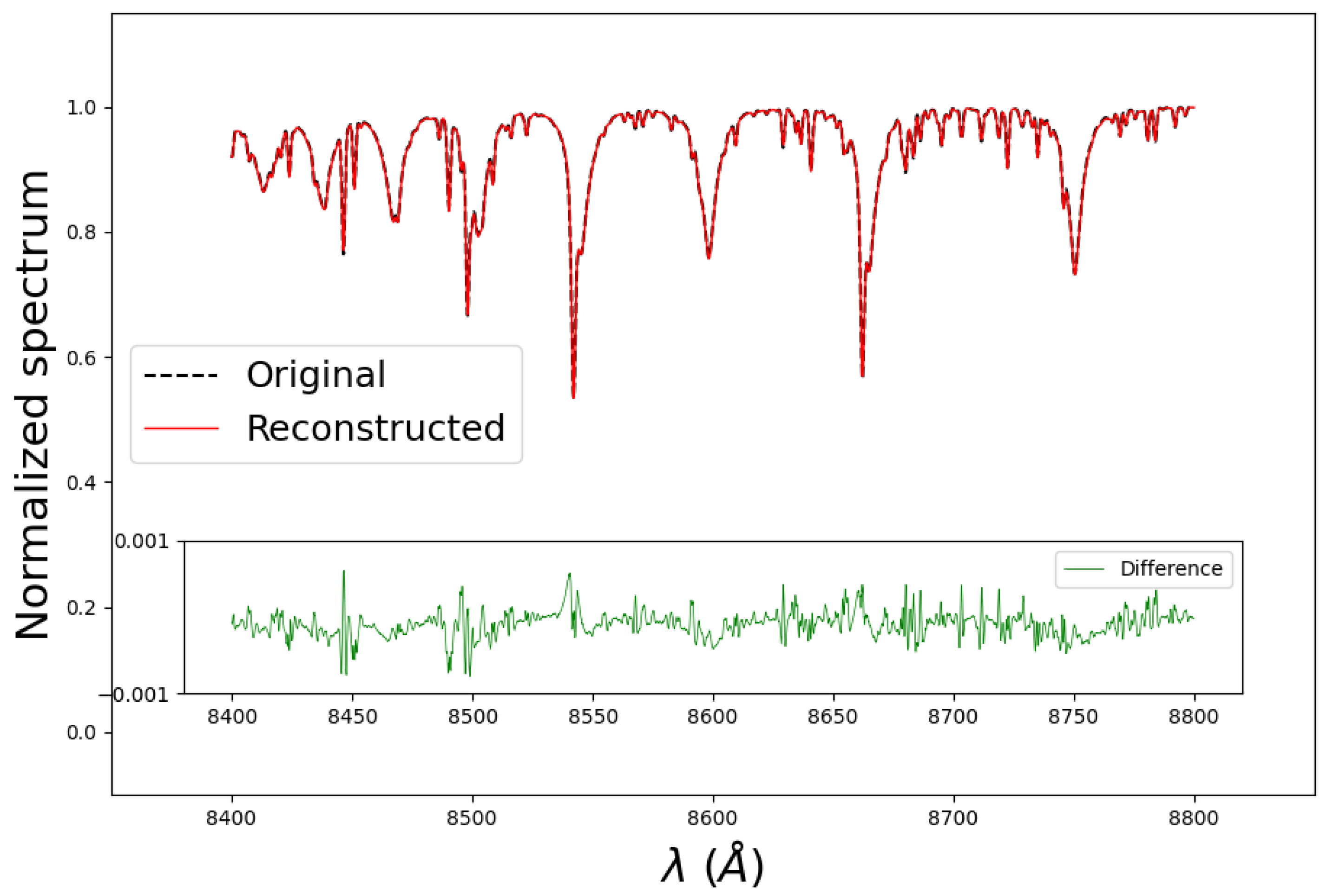
Convergence is set when a monitored metric stops improving during training. This stopping criterion is set to be at 15 iterations of non-improvement. Around 75 iterations are required to reach a minimum loss function. Figure 3 shows the behavior of the Training and Validation loss as a function of the first 50 epochs. We have used the “Adam” optimizer combined with a Mean Squared Error (MSE) loss function. The precision was verified using different metrics such as the MSE, which is found to be , a Mean Absolute Error (MAE) of 0.0013, a variance score of 0.998, and an R2 score of 0.999. A better way to grasp the accuracy is to display an original spectrum along its reconstructed one. Figure 4 displays the transformation of a synthetic spectrum that is not included in the training database. The original spectrum (in dashed black lines) passes through the autoencoder in order to be encoded and then decoded. The decoded spectrum is shown in red, and the difference between the original and decoded spectrum is shown in green. On average, the reconstruction is achieved with an error <0.1%.
2.3. Fully Connected Neural Network
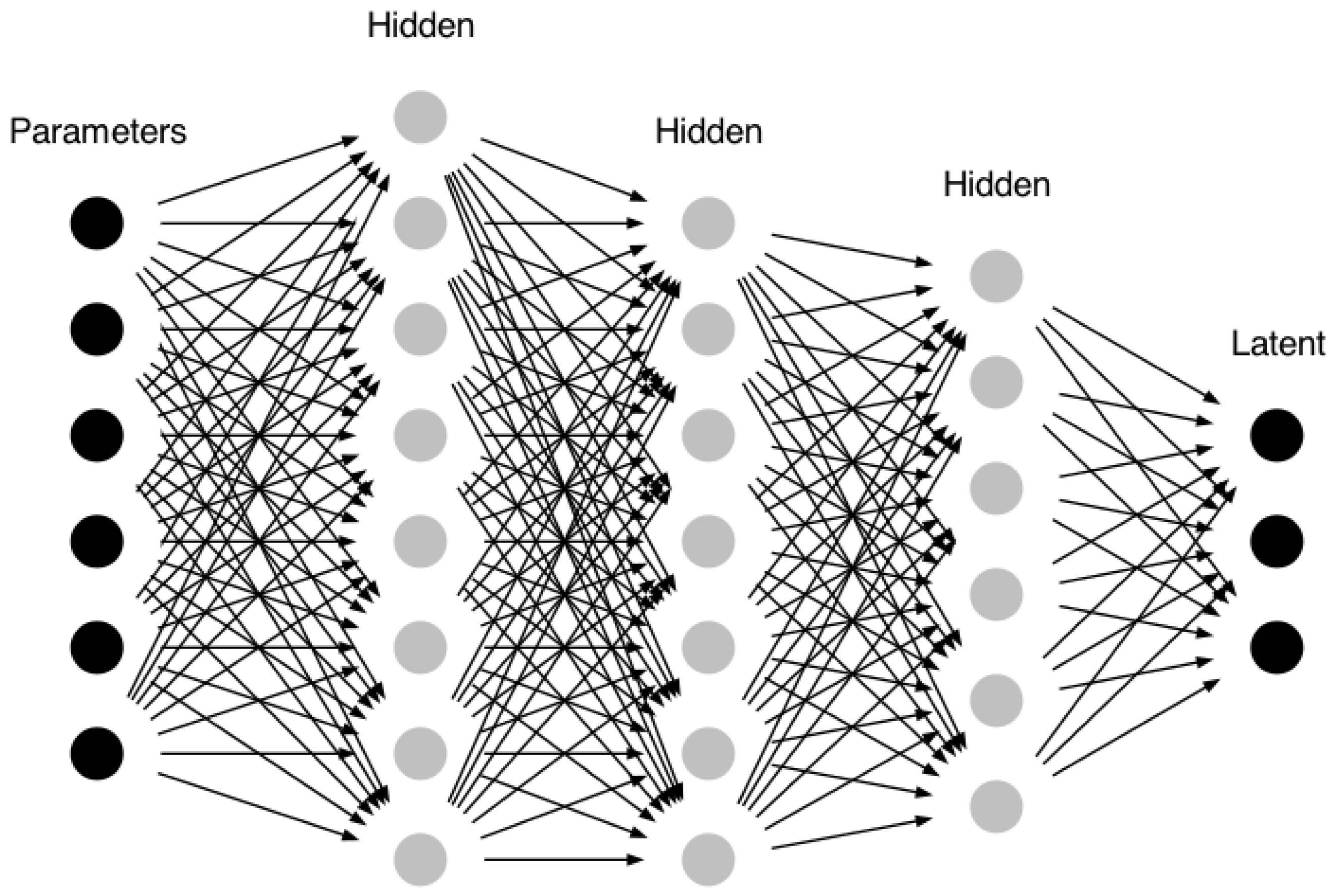
The next step of this technique is to link the stellar parameters (, , , , and ), and the resolution of the learning database to the Latent Space through a Fully Connected Neural Network. Using the same database as Section 2.2, we have trained this model by linking the stellar labels of the database to the Latent Space of the same database. This Latent Space is found by passing the spectra database through the encoder part of the autoencoder. This means that the Latent Space is the common link between the autoencoder and the Fully Connected Neural Network. In the first case, the Latent Space is the output of the encoder part and in the second, the same Latent Space is a transformation of the stellar labels. The architecture of the NN is shown in Figure 5 and the characteristic of each layer is displayed in Table 3. We have used “Adamax” as optimizer and an MSE loss function. Input data were divided into batches of 512 spectra per batch. The learning database was divided into 80% for training and 20% for validation.
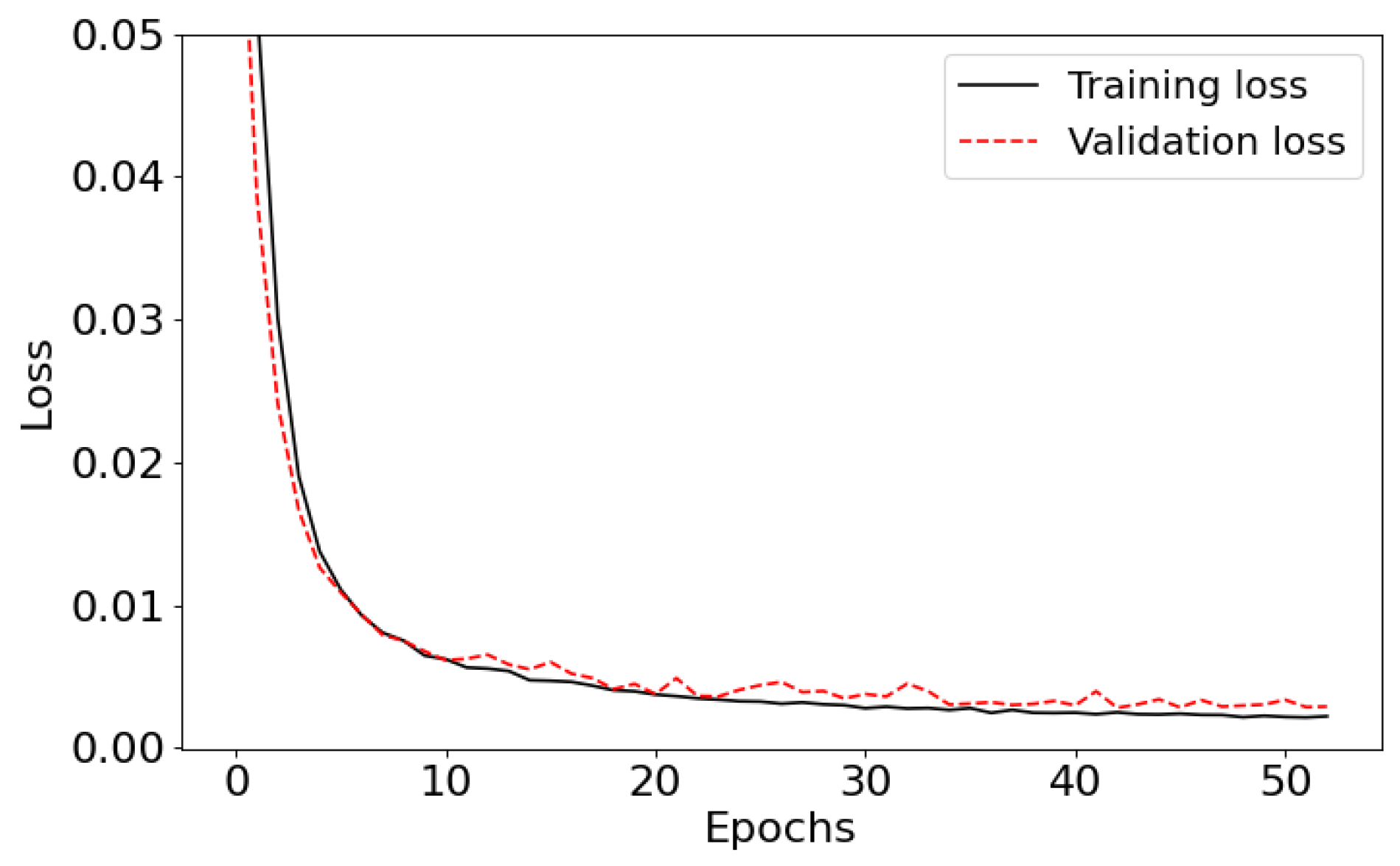
The training of the model stops when the loss does not decrease significantly after 15 iterations. The NN requires 50–60 iterations for the loss function to reach a minimum value (i.e., the stopping criterion). This minimum is for both the training and validation databases. Figure 6 shows the variation of the Training and Validation loss function as a function of the epochs number. The evaluation of this step is not straightforward. Detailed inspections were performed to make sure that no under- or overfitting is occurring. In the next section (Section 2.4), we will be using this Fully connected network in combination with the decoder of Section 2.2 to generate spectra based on input stellar parameters.
2.4. Connecting Both Networks
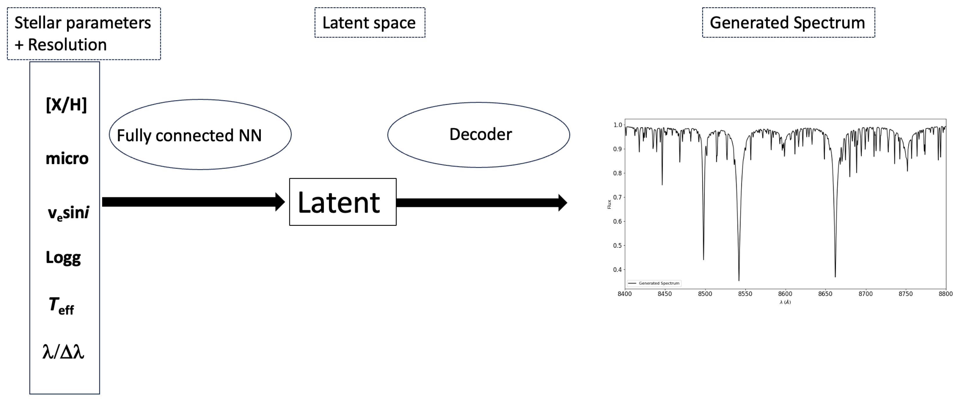
The final step is to combine the Fully connected Neural Network of Section 2.3 and the decoder part of Section 2.2 to generate new data. The main purpose is that the user will input five stellar parameters and a resolution as input and obtain a newly normalized generated spectrum of 4000 data points between 8400 and 8800 Å.
By providing a set of stellar parameters, we can apply the Fully Connected Neural Network of Section 2.3 to derive the 10 data points output that will be used a Latent Space. These 10 points are then used as input for the decoder part and decoding them will result in a generated synthetic spectrum of 4000 data points. The flowchart of this procedure is shown in Figure 7. Mathematically, the generated synthetic spectrum is calculated as follows:
where “Stellar Labels” have a dimension of 6, NN(Stellar Labels) a dimension of 10, and decoder(NN(Stellar Labels)) a dimension of 4000. In the next section (Section 3), we will test the accuracies of the generated spectra and compare them, through different metrics, to spectra calculated using SYNSPEC.
3. Results
The evaluation of the quality of the generated spectra is conducted in two steps. First, The generated spectra were visually inspected along with the ones calculated using SYNSPEC. Second, we performed a detailed stellar parameters analysis of the generated spectra in order to constrain their use in stellar spectroscopy.
3.1. Generated Spectra
A set of ∼5000 generated spectra was computed using stellar parameters and resolution chosen randomly in the range of Table 1. These spectra do not belong to the training database that was used in the autoencoder or the one in the Fully Dense Neural Network.
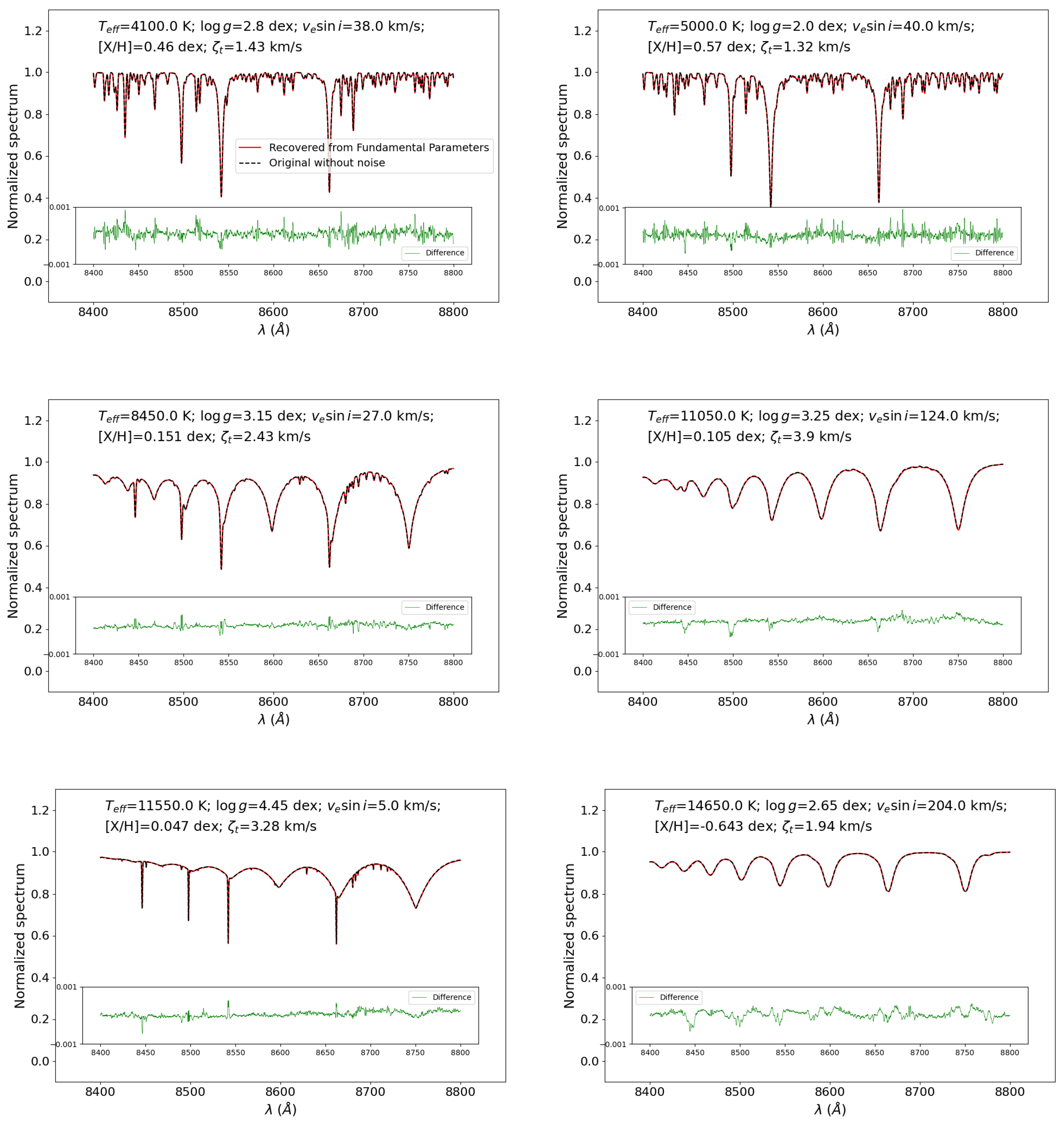
Qualitatively, the generated spectra are compared to synthetic spectra calculated using SYNSPEC with the same stellar parameters and resolution. Figure 8 represents a sample of generated plots with each one displaying a generated spectrum (red line) compared to SYNSPEC synthetic spectrum (black dashed line), which has both the same stellar parameter and a resolution of 11,500. The green dashed lines in the figure represent the difference between the generated and the synthetic spectra. One synthetic spectrum requires a calculation time of ∼3 min with SYNSPEC whereas a generated spectrum using the combination of NN and decoder requires ∼9 ms with the same platform. This step shows that we were able to reconstruct the spectra with detailed line profiles for all combinations of stellar parameters.
3.2. Stellar Parameters
A quantitative evaluation of the generated spectra is conducted by inferring the stellar parameters of these spectra. Once the parameters are derived, we compare them to the original parameters used to construct these spectra. The stellar parameters will be, in that case, derived with an NN trained with SYNSPEC synthetic data. The main goal is to find that the derived stellar parameters have accuracies in the order of the one found when applying the same technique on SYNSPEC synthetic spectra. In that case, the reconstruction generative technique is shown to be able to reproduce the data as if they are calculated using the radiative transfer code.
We start by developing an NN that derives the six parameters (, , , , , and resolution). The network is based on the work of [2,3] and involves a preprocessing of the original spectra using a PCA transformation. The input data consist of a matrix of synthetic data having a dimension of 205,000 spectra × 4000 wavelength points. This matrix is reduced to 205,000 spectra × 15 PCA coefficients. As explained in [3], this step is optional but recommended to increase the speed of the calculations. The choice of the number of coefficients is regulated by the PCA reconstructed error. We found that by retaining only 15 parameters, we were able to reduce the mean reconstructed error of the training database to a value of ≤0.5% (see also [28] and [1], for an explanation about the choice of the number of Principal Components).
The PCA coefficients are used instead of the synthetic spectra in the NN. The NN is then trained to relate these 15 coefficients to the five stellar parameters and resolution according to the architecture displayed in Table 4. This network is directly adapted from [3] and is used for every stellar parameter, independently. The training PCA database is divided into 80% for training and 20% for validation. An additional several tens of thousands of synthetic spectra were calculated for the purpose of being used as test data. The same PCA transformation was used on these test data to derive the 15 coefficients per test spectrum.
In this work, we were able to optimize the network for all stellar parameters using a single set of hyperparameters. This means that the network is the same whether we train for , , or any other parameter. The details about the layers are displayed in Table 4. A kernel initializer of “Random Normal”, combined with an optimizer of “Adamax” and an “MSE” loss function were used. The input data were divided into batches of 512 spectra (PCA coefficients) per batch. Finally, the loss function reaches a minimum after ∼75–200 iterations, depending on the stellar parameter.
The accuracies of the stellar parameters found in this analysis are shown in Table 5. These values are calculated as MSE between the original true parameter of the spectra and the ones derived from the NN. Quantitatively, the main result that plays a role in our work is the comparison between the accuracies of the test data and the reconstructed generated data. This comparison shows how accurate the generated spectra using NN/decoder are with respect to the ones calculated using the radiative transfer code SYNSPEC. Of course, none of the sets of test and generated data were used in the training of the NNs.
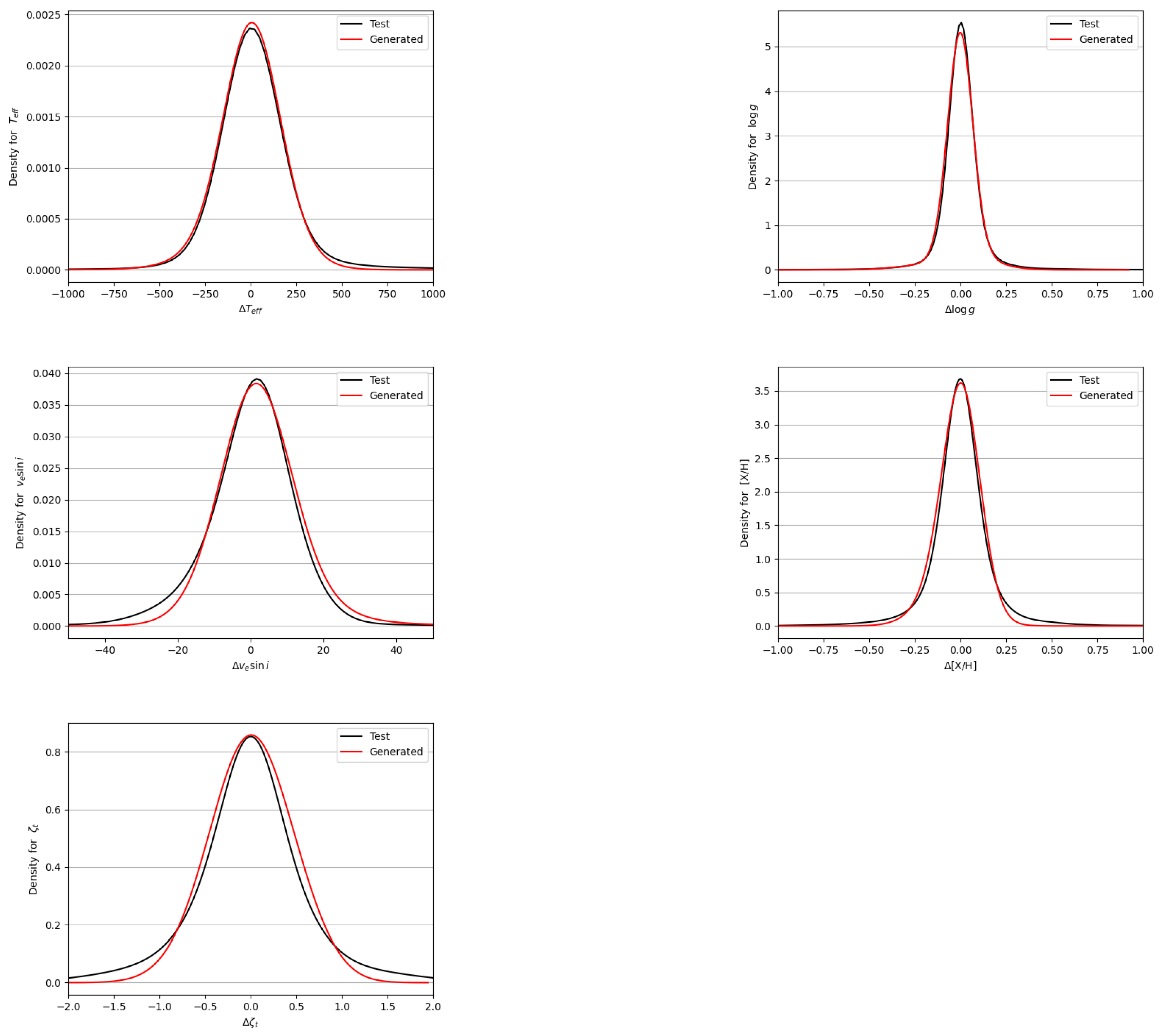
We found that the accuracies on the stellar parameters for the generated spectra (column 5 of Table 5) are in the same order as the ones of the synthetic spectra calculated with SYNCPEC (Test data, column 4 Table 5). These results show that the generative technique is capable of reproducing the flux with all the line profiles and intensities. For a specific stellar parameter, the behavior of the accuracy as a function of the parameter is identical for both synthetic data (SYNSPEC) and generated ones (NN and decoder). In Figure 9, we represent the density distributions of the difference between the predicted and the true values of , , , , and , for the synthetic Test (black) and generated data (red). The Generated data behave similarly to synthetic ones; the flux, line profiles, and characteristics are identical to the one calculated using radiative transfer codes.
4. Discussion and Conclusions
In this work, we have developed a technique, based on deep learning, that takes stellar parameters as input and delivers a generated spectrum as an output. The network is trained using a set of synthetic spectra calculated using the SYNSPEC radiative transfer code and ATLAS9 model atmospheres. We were able to generate spectra of BAFGK stars having different surface gravity (), projected equatorial rotational velocity (), metallicity (), microturbulent velocity (), and at a resolution around 11,500. The choice of the wavelength range (8400–8800 Å) and resolution is related to the fact that we were trying to mimic RVS spectra. We showed that this technique is capable of reproducing the flux and line profiles of stars. Deriving the stellar parameters of the generated spectra shows that the found accuracies are identical to the ones using classical synthetic spectra.
In this procedure, we are not constraining the technique of deriving the stellar parameters, rather we are constraining the spectra generation procedure. The astronomical community uses a large number of stellar parameter determination techniques, most of them based on synthetic data. An example is the GSP-Spec [25] used in the context of Gaia RVS spectra and requires a set of MARCS models and the use of TURBOSPECTRUM radiative transfer code. Our work shows that instead of using synthetic spectra, users can train new models based on the stellar range they need for their project, and generate new stellar spectra to be used in their parameter derivation techniques. The training could be conducted using spectra from available online databases that are usually calculated with large steps in and . Such databases are POLLUX [16], TLUSTY ([17], PHOENIX [15], and the AMBRE database [18]. Most of these databases contain standard LTE spectra. Training the networks with Non-LTE spectra will result in a more accurate spectra reconstruction and more reliable results when these generated spectra are used to parametrize true observations.
Eventually, our models should be trained on observed stars with well-known fundamental parameters (i.e., Benchmark stars). Training the model with observed data and for specific stellar ranges will result in generating a large number of spectra that can be used in the purpose of analysis of large surveys such as RAVE [29], the Gaia-ESO Survey [30], LAMOST [31], APOGEE [32], and GALAH [33]. For a large wavelength range, we can mention the Melchiors3 database [34] that combines ∼3250 high signal-to-noise spectra of O to M stars between 3900 and 9000 Å and having a spectral resolution of 85,000. The generalization of the model presented here is very challenging for observational astronomy. It will require the combination of several surveys with an inspection of every star in terms of the quality of the spectrum and the amount of available stellar labels per star.
The next step of this project is to apply the reconstructing technique to a large database containing a wide wavelength range (3000–7000 Å), a large range of spectral resolutions ( between 1000 and 150,000), and for BAFGKM stars at different evolutionary stages. Having a large spectral resolution will allow the user to generate spectra for a large range of on-ground and space observations. SYNSPEC allows the modifications of individual abundances up to Z = 99. We will also be modifying individual chemical abundances instead of the overall metallicity in order to be able to generate spectra with any combination of abundances. Adding to that the range in and , we estimate the size of one database to be in the order of several terabytes. This will require several months of training on our current machines. Once the network is optimized in terms of hyperparameters and architecture, it will be available freely to the scientific community along with a detailed tutorial. Finally, we are currently investigating the relation between the number of spectra in the training database and the wavelength range size. This will allow us to construct databases with optimized number of spectra leading to a significant gain in calculation time.
Funding
This research received no external funding.
Acknowledgments
The author acknowledges Saint Mary’s College for providing the necessary computational power for the success of this project. The author thanks Ian Bentley, Frédéric Paletou, and Hikmat Farhat for their helpful comments and suggestions.
Conflicts of Interest
The authors declare no conflict of interest.
| 1 | https://www.tensorflow.org/ (accessed on 15 October 2023). |
| 2 | https://keras.io/ (accessed on 15 October 2023). |
| 3 | https://www.royer.se/melchiors.html (accessed on 10 November 2023). |
References
- Gebran, M.; Farah, W.; Paletou, F.; Monier, R.; Watson, V. A new method for the inversion of atmospheric parameters of A/Am stars. A&A 2016, 589, A83. [Google Scholar] [CrossRef]
- Gebran, M.; Connick, K.; Farhat, H.; Paletou, F.; Bentley, I. Deep learning application for stellar parameters determination: I-constraining the hyperparameters. Open Astron. 2022, 31, 38. [Google Scholar] [CrossRef]
- Gebran, M.; Paletou, F.; Bentley, I.; Brienza, R.; Connick, K. Deep learning applications for stellar parameter determination: II-application to the observed spectra of AFGK stars. Open Astron. 2023, 32, 209. [Google Scholar] [CrossRef]
- Gilda, S. Deep-REMAP: Parameterization of Stellar Spectra Using Regularized Multi-Task Learning. arXiv 2023, preprint. arXiv:2311.03738. [Google Scholar]
- Kassounian, S.; Gebran, M.; Paletou, F.; Watson, V. Sliced Inverse Regression: Application to fundamental stellar parameters. Open Astron. 2019, 28, 68. [Google Scholar] [CrossRef]
- Gustafsson, B.; Edvardsson, B.; Eriksson, K.; Jørgensen, U.G.; Nordlund, Å.; Plez, B. A grid of MARCS model atmospheres for late-type stars. A&A 2008, 486, 951. [Google Scholar] [CrossRef]
- Plez, B. Astrophysics Source Code Library, Record Ascl:1205.004. 2012. Available online: https://ui.adsabs.harvard.edu/abs/2012ascl.soft05004P (accessed on 15 October 2023).
- Sneden, C.; Bean, J.; Ivans, I.; Lucatello, S.; Sobeck, J. 2012, Astrophysics Source Code Library, Record Ascl:1202.009. Available online: https://ui.adsabs.harvard.edu/abs/2012ascl.soft02009S (accessed on 15 October 2023).
- Kurucz, R.L. model atmospheres for population synthesis. Symp. Int. Astron. Union 1992, 149, 225. [Google Scholar]
- Sbordone, L.; Bonifacio, P.; Castelli, F.; Kurucz, R.L. ATLAS and SYNTHE under Linux. arXiv 2004, preprint. arXiv:astro-ph/0406268. [Google Scholar] [CrossRef]
- Piskunov, N.; Valenti, J.A. Spectroscopy Made Easy: Evolution. A&A 2017, 597, A16. [Google Scholar] [CrossRef]
- Hubeny, I.; Lanz, T. Astrophysics Source Code Library, 2011, Record Ascl:1109.022. Available online: https://ui.adsabs.harvard.edu/abs/2011ascl.soft09022H (accessed on 15 October 2023).
- Hubeny, I.; Lanz, T. A brief introductory guide to TLUSTY and SYNSPEC. arXiv 2017, preprint. arXiv:1706.01859. [Google Scholar] [CrossRef]
- Hubeny, I.; Allende Prieto, C.; Osorio, Y.; Lanz, T. TLUSTY and SYNSPEC Users’s Guide IV: Upgraded Versions 208 and 54. arXiv 2021, preprint. arXiv:2104.02829. [Google Scholar] [CrossRef]
- Husser, T.-O.; Berg, W.; Dreizler, S.; Homeier, D.; Reiners, A.; Barman, T.; Hauschildt, P.H. A new extensive library of PHOENIX stellar atmospheres and synthetic spectra. A&A 2013, 553, A6. [Google Scholar] [CrossRef]
- Palacios, A.; Gebran, M.; Josselin, E.; Martins, F.; Plez, B.; Belmas, M.; Lèbre, A. POLLUX: A database of synthetic stellar spectra. A&A 2010, 516, A13. [Google Scholar] [CrossRef]
- Lanz, T.; Hubeny, I. A Grid of Non-LTE Line-blanketed Model Atmospheres of O-Type Stars. Astrophys. J. Suppl. Ser. 2003, 146, 417. [Google Scholar] [CrossRef]
- de Laverny, P.; Recio-Blanco, A.; Worley, C.C.; Plez, B. The AMBRE project: A new synthetic grid of high-resolution FGKM stellar spectra. A&A 2012, 544, A126. [Google Scholar] [CrossRef]
- Cropper, M.; Katz, D.; Sartoretti, P.; Prusti, T.; de Bruijne, J.H.J.; Chassat, F.; Charvet, P.; Boyadjian, J.; Perryman, M.; Sarri, G.; et al. Gaia Data Release 2. Gaia Radial Velocity Spectrometer. A&A 2018, 616, A5. [Google Scholar] [CrossRef]
- Vallenari, A.; Brown, A.G.A.; Prusti, T.; de Bruijne, J.H.J.; Arenou, F.; Babusiaux, C.; Creevey, O.L.; Ducourant, C.; Evans, D.W.; Eyer, L.; et al. [Gaia Collaboration] Gaia Data Release 3. Summary of the content and survey properties. A&A 2023, 674, A1. [Google Scholar] [CrossRef]
- Recio-Blanco, A.; de Laverny, P.; Allende Prieto, C.; Fustes, D.; Manteiga, M.; Arcay, B.; Bijaoui, A.; Dafonte, C.; Ordenovic, C.; Blanco, D.O. Stellar parametrization from Gaia RVS spectra. A&A 2016, 585, A93. [Google Scholar] [CrossRef]
- Castelli, F.; Kurucz, R.L. New Grids of ATLAS9 Model Atmospheres. arXiv 2003, preprint. arXiv:astro-ph/0405087. [Google Scholar] [CrossRef]
- Smalley, B. Observations of convection in A-type stars. Proc. Int. Astron. Union 2004, 224, 131. [Google Scholar] [CrossRef]
- Grevesse, N.; Sauval, A.J. Standard Solar Composition. Space Sci. Rev. 1998, 85, 161. [Google Scholar] [CrossRef]
- Recio-Blanco, A.; de Laverny, P.; Palicio, P.A.; Kordopatis, G.; Álvarez, M.A.; Schultheis, M.; Contursi, G.; Zhao, H.; Torralba Elipe, G.; Ordenovic, C.; et al. Gaia Data Release 3. Analysis of RVS spectra using the General Stellar Parametriser from spectroscopy. A&A 2023, 674, A29. [Google Scholar] [CrossRef]
- Einig, L.; Pety, J.; Roueff, A.; Vandame, P.; Chanussot, J.; Gerin, M.; Orkisz, J.H.; Palud, P.; Santa-Maria, M.G.; Magalhaes, V.d.S.; et al. Deep learning denoising by dimension reduction: Application to the ORION-B line cubes. A&A 2023, 677, A158. [Google Scholar] [CrossRef]
- Scourfield, M.; Saintonge, A.; de Mijolla, D.; Viti, S. De-noising of galaxy optical spectra with autoencoders. Mon. Not. R. Astron. Soc. 2023, 526, 3037. [Google Scholar] [CrossRef]
- Paletou, F.; Böhm, T.; Watson, V.; Trouilhet, J.-F. Inversion of stellar fundamental parameters from ESPaDOnS and Narval high-resolution spectra. A&A 2015, 573, A67. [Google Scholar] [CrossRef]
- Steinmetz, M.; Zwitter, T.; Siebert, A.; Watson, F.G.; Freeman, K.C.; Munari, U.; Campbell, R.; Williams, M.; Seabroke, G.M.; Wyse, R.F.; et al. The Radial Velocity Experiment (RAVE): First Data Release. Astron. J. 2006, 132, 1645. [Google Scholar] [CrossRef]
- Gilmore, G.; Randich, S.; Asplund, M.; Binney, J.; Bonifacio, P.; Drew, J.; Feltzing, S.; Ferguson, A.; Jeffries, R.; Micela, G.; et al. The Gaia-ESO public spectroscopic survey. Messenger 2012, 147, 25. [Google Scholar]
- Zhao, G.; Zhao, Y.-H.; Chu, Y.-Q.; Jing, Y.-P.; Deng, L.-C. LAMOST spectral survey—An overview. Res. Astron. Astrophys. 2012, 12, 723. [Google Scholar] [CrossRef]
- Majewski, S.R.; Schiavon, R.P.; Frinchaboy, P.M.; Prieto, C.A.; Barkhouser, R.; Bizyaev, D.; Blank, B.; Brunner, S.; Burton, A.; Carrera, R.; et al. The Apache Point Observatory Galactic Evolution Experiment (APOGEE). Astron. J. 2017, 154, 94. [Google Scholar] [CrossRef]
- Martell, S.L.; Sharma, S.; Buder, S.; Duong, L.; Schlesinger, K.J.; Simpson, J.; Lind, K.; Ness, M.; Marshall, J.P.; Asplund, M.; et al. The GALAH survey: Observational overview and Gaia DR1 companion. Mon. Not. R. Astron. Soc. 2017, 465, 3203. [Google Scholar] [CrossRef]
- Royer, P.; Merle, T.; Dsilva, K.; Sekaran, S.; Van Winckel, H.; Frémat, Y.; Van der Swaelmen, M.; Gebruers, S.; Tkachenko, A.; Laverick, M.; et al. MELCHIORS: The Mercator Library of High Resolution Stellar Spectroscopy. arXiv 2023, preprint. arXiv:2311.02705. [Google Scholar] [CrossRef]
Figure 1.
Left: Color map representing the fluxes for a sample of the training database. Wavelengths are in Å. Right: Example of a synthetic spectrum not calculated in the RVS wavelength range.
Figure 1.
Left: Color map representing the fluxes for a sample of the training database. Wavelengths are in Å. Right: Example of a synthetic spectrum not calculated in the RVS wavelength range.

Figure 2.
General display of an autoencoder that transforms an input spectrum to a lower dimension using a series of hidden layers and then reconstructs it with its original dimension. The middle layer is the Latent Space that contains the reduced spectrum.
Figure 2.
General display of an autoencoder that transforms an input spectrum to a lower dimension using a series of hidden layers and then reconstructs it with its original dimension. The middle layer is the Latent Space that contains the reduced spectrum.

Figure 3.
Training and validation loss with respect to the epoch number during the learning process of the autoencoder. Only the first 50 epochs are shown.
Figure 3.
Training and validation loss with respect to the epoch number during the learning process of the autoencoder. Only the first 50 epochs are shown.

Figure 4.
Reconstruction of a synthetic spectrum using the autoencoder of Table 2. The original spectrum is in black, the reconstructed one is in red, and the difference between them is in green.
Figure 4.
Reconstruction of a synthetic spectrum using the autoencoder of Table 2. The original spectrum is in black, the reconstructed one is in red, and the difference between them is in green.

Figure 5.
General display of the Fully Connected Neural Network that related the five stellar parameters per spectrum and the resolution to the Latent Space. Six parameters are introduced as input and pass through a series of hidden layers until reaching an output containing the encoded part of the learning database and having the dimension of 10 data points per spectrum.

Figure 6.
Training and validation loss with respect to the epoch number during the learning process of the Fully Connected Neural Network that related the stellar labels to the Space.
Figure 6.
Training and validation loss with respect to the epoch number during the learning process of the Fully Connected Neural Network that related the stellar labels to the Space.

Figure 7.
Flowchart of the general steps to generate a synthetic spectrum.

Figure 8.
Generated spectra (red) compared to the ones calculated using SYNEPC (black) having the same combination of stellar parameters and resolution. The green dashed lines represent the difference between the generated spectra and the synthetic ones. Each spectrum has a different combination of stellar parameters , , , , and .

Figure 9.
Density distribution of the difference between the predicted values of a stellar label and the true values for the synthetic (black) and generated data (red).
Figure 9.
Density distribution of the difference between the predicted values of a stellar label and the true values for the synthetic (black) and generated data (red).


Table 1.
Range of parameters used in the calculation of the synthetic spectra. The upper part of the table displays the astrophysical parameters of the stars whereas the bottom one displays the instrumental one. All these spectra were calculated in a wavelength range of 8400–8800 Å.
Table 1.
Range of parameters used in the calculation of the synthetic spectra. The upper part of the table displays the astrophysical parameters of the stars whereas the bottom one displays the instrumental one. All these spectra were calculated in a wavelength range of 8400–8800 Å.
| Parameter | Range |
|---|---|
| 3600–15,000 K | |
| 2.0–5.0 dex | |
| 0–300 km/s | |
| −1.5–1.5 dex | |
| 0–4 km/s | |
| Resolution () | 5000–14,500 |
Table 2.
Architecture of the autoencoder used in this work.
| Layer | Characteristics | Activation Function |
|---|---|---|
| Encoder | ||
| Input | Spectrum of 4000 data points | – |
| Hidden | 1024 neurons | relu |
| Hidden | 512 neurons | relu |
| Hidden | 256 neurons | relu |
| Hidden | 64 neurons | relu |
| Hidden | 32 neurons | relu |
| Latent Space | 10 neurons | relu |
| Decoder | ||
| Hidden | 32 neurons | relu |
| Hidden | 64 neurons | relu |
| Hidden | 256 neurons | relu |
| Hidden | 512 neurons | relu |
| Hidden | 1024 neurons | relu |
| Output | Reconstructed spectrum of 4000 data points | – |
Table 3.
Architecture of the Fully Connected Neural Network used to relate the stellar parameters and resolution to the Latent Space.
Table 3.
Architecture of the Fully Connected Neural Network used to relate the stellar parameters and resolution to the Latent Space.
| Layer | Characteristics | Activation Function |
|---|---|---|
| Input | Stellar parameters + resolution (six data points per spectrum) | – |
| Hidden | 5000 neurons | relu |
| Dropout | 30% | – |
| Hidden | 2000 neurons | relu |
| Dropout | 30% | – |
| Hidden | 512 neurons | relu |
| Dropout | 30% | – |
| Hidden | 32 neurons | relu |
| Output | Latent Space of 10 data points | – |
Table 4.
Architecture of the Fully Connected Neural Network used to relate the PCA coefficients to stellar parameters.
Table 4.
Architecture of the Fully Connected Neural Network used to relate the PCA coefficients to stellar parameters.
| Layer | Characteristics | Activation Function |
|---|---|---|
| Input | PCA coefficient (15 data points per spectrum) | – |
| Hidden | 5000 neurons | relu |
| Hidden | 2000 neurons | relu |
| Hidden | 1000 neurons | relu |
| Hidden | 512 neurons | relu |
| Hidden | 64 neurons | relu |
| Output | Stellar Parameters (six data points per spectrum) | – |
Table 5.
Derived accuracies of the stellar parameters for the training, validation, test, and generated database.
Table 5.
Derived accuracies of the stellar parameters for the training, validation, test, and generated database.
| Parameter | Training | Validation | Test | Generated |
|---|---|---|---|---|
| (K) | 70 | 110 | 120 | 119 |
| (dex) | 0.02 | 0.03 | 0.03 | 0.05 |
| (Km/s) | 5.0 | 6.0 | 6.5 | 7.0 |
| (dex) | 0.04 | 0.08 | 0.15 | 0.15 |
| (Km/s) | 0.15 | 0.17 | 0.17 | 0.20 |
Disclaimer/Publisher’s Note: The statements, opinions and data contained in all publications are solely those of the individual author(s) and contributor(s) and not of MDPI and/or the editor(s). MDPI and/or the editor(s) disclaim responsibility for any injury to people or property resulting from any ideas, methods, instructions or products referred to in the content. |
© 2024 by the author. Licensee MDPI, Basel, Switzerland. This article is an open access article distributed under the terms and conditions of the Creative Commons Attribution (CC BY) license (https://creativecommons.org/licenses/by/4.0/).
Share and Cite
MDPI and ACS Style
Gebran, M. Generating Stellar Spectra Using Neural Networks. Astronomy 2024, 3, 1-13. https://doi.org/10.3390/astronomy3010001
AMA Style
Gebran M. Generating Stellar Spectra Using Neural Networks. Astronomy. 2024; 3(1):1-13. https://doi.org/10.3390/astronomy3010001
Chicago/Turabian StyleGebran, Marwan. 2024. "Generating Stellar Spectra Using Neural Networks" Astronomy 3, no. 1: 1-13. https://doi.org/10.3390/astronomy3010001