Review

Quantum Astronomy at the University and INAF Astronomical Observatory of Padova, Italy

by
Cesare Barbieri
1,2,*,†,
Giampiero Naletto
1,2 and
Luca Zampieri
2
1
Department of Physics and Astronomy “G. Galilei”, University of Padova, 35131 Padova, Italy
2
INAF-Astronomical Observatory of Padova, 35122 Padova, Italy
*
Author to whom correspondence should be addressed.
Emeritus of Astronomy.
Astronomy 2023, 2(3), 180-192; https://doi.org/10.3390/astronomy2030013
Submission received: 24 April 2023 / Revised: 26 July 2023 / Accepted: 7 August 2023 / Published: 23 August 2023
(This article belongs to the Special Issue Quantum Astronomy)

Abstract

:
Twenty years ago, we started to apply quantum optics to the astronomical research carried out inside the Department of Physics and Astronomy and the INAF Astronomical Observatory in Padova, Italy. The initial activities were stimulated by the project of the European Southern Observatory (ESO) to build a 100 m diameter telescope, the Overwhelmingly Large (OWL) telescope. The enormous photon flux expected from such an aperture suggested that quantum optics concepts be utilized in order to obtain novel astrophysical results. Following initial successful attempts to utilize the orbital angular momentum of the light beam to enhance the visibility of faint companions to bright stars, the Padova team concentrated its efforts on very high time resolution, in order to measure and store the arrival time of celestial photons to better than one nanosecond. To obtain observational results, we built two photon counting photometers (AquEye and IquEye) to be used with our telescopes of the Asiago Observatory and with 4 m class telescopes such as the ESO New Technology Telescope (NTT) in Chile. This paper firstly describes these two instruments and then expounds the results obtained on pulsar light curves, lunar occultations and the first photon counting intensity interferometry measurements of the bright star Vega. Indeed, the correlation of photon arrival times on two or more apertures can lead to extremely high angular resolutions, as shown around 1970 by Hanbury Brown and Twiss. Prospects for quantum intensity interferometry with arrays of Cherenkov light telescopes will also be described.

1. Introduction

At the beginning of the 21st century, the European Southern Observatory (ESO) started the design of a 100 m aperture telescope, the Overwhelmingly Large telescope (OWL). The enormous number of photons collected by such a giant area supported the hope of applying quantum optics concepts to analyze the light from celestial objects from a new perspective, in order to derive novel information about the nature of the different sources of light, from thermal to synchrotron to naturally lased ones, and the effects of a medium in the intervening path to the observer. Motivated by such hope, a team of European astronomers, supported by an ESO contract, produced a first fundamental document, QuantEye (The Quantum Eye of OWL, see [1,2]) which constitutes the basis of quantum astronomy (see also [3,4]). The OWL project was discontinued due to technical and financial difficulties and was superseded by the 39 m Extremely Large telescope (ELT), now in advanced construction on Cerro Armazones in Chile. The ELT will still be the largest in the world, and many of the considerations expounded in QuantEye maintain their validity. That document contains not only a theoretical discussion of astrophysical problems but also the conceptual description of a quantum photometer capable of coming close to the time–energy limits imposed by the Heisenberg uncertainty principle. Possible solutions, consistent with the available technology, for the optical design, photon receiver, time of arrival acquisition, storage and analysis were indicated.
Out of the many themes deserving a quantum treatment, the team of astronomers, physicists and engineers of the Department of Physics and Astronomy of the University of Padova and of INAF Astronomical Observatory of Padova concentrated their attention on very high angular and time resolutions. Taking advantage of the availability of telescopes in Asiago (the 1.22 m Galileo at Asiago Pennar and the 1.82 m Copernicus at Asiago Cima Ekar), instruments were built to test with real observations the conceptual design indicated in QuantEye. Successful experiments with the orbital angular momentum (OAM) were carried out with the Galileo telescope [5,6,7]. These experiments attracted great attention (paper [6] was selected among the highlights of the Astronomy & Astrophysics journal for that year), and the overview paper on 30 years of OAM [8] contains a citation of such works. However, due to a lack of resources, this line has been interrupted, at least for the moment. In parallel, we concentrated our efforts on very high time resolution astronomy. In this review paper we describe the results obtained with our instruments on very high time resolution of optical pulsar light curves and lunar occultations. We also show that correlating the arrival times of photons on two or more apertures reintroduces the possibility of realizing high spatial resolution measurements via the technique of intensity interferometry pioneered by Hanbury Brown and Twiss in the 1970s [9], and, in the final chapter, we illustrate our experiment with intensity interferometry of the bright star Vega using the two Asiago telescopes.

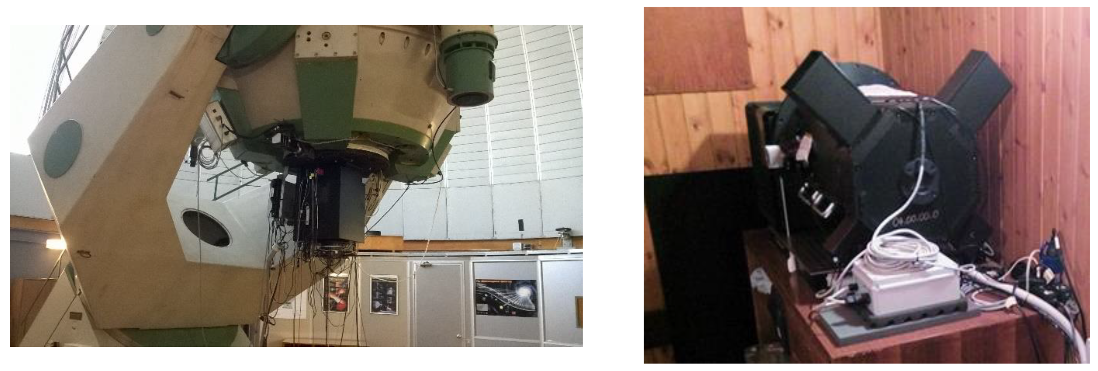
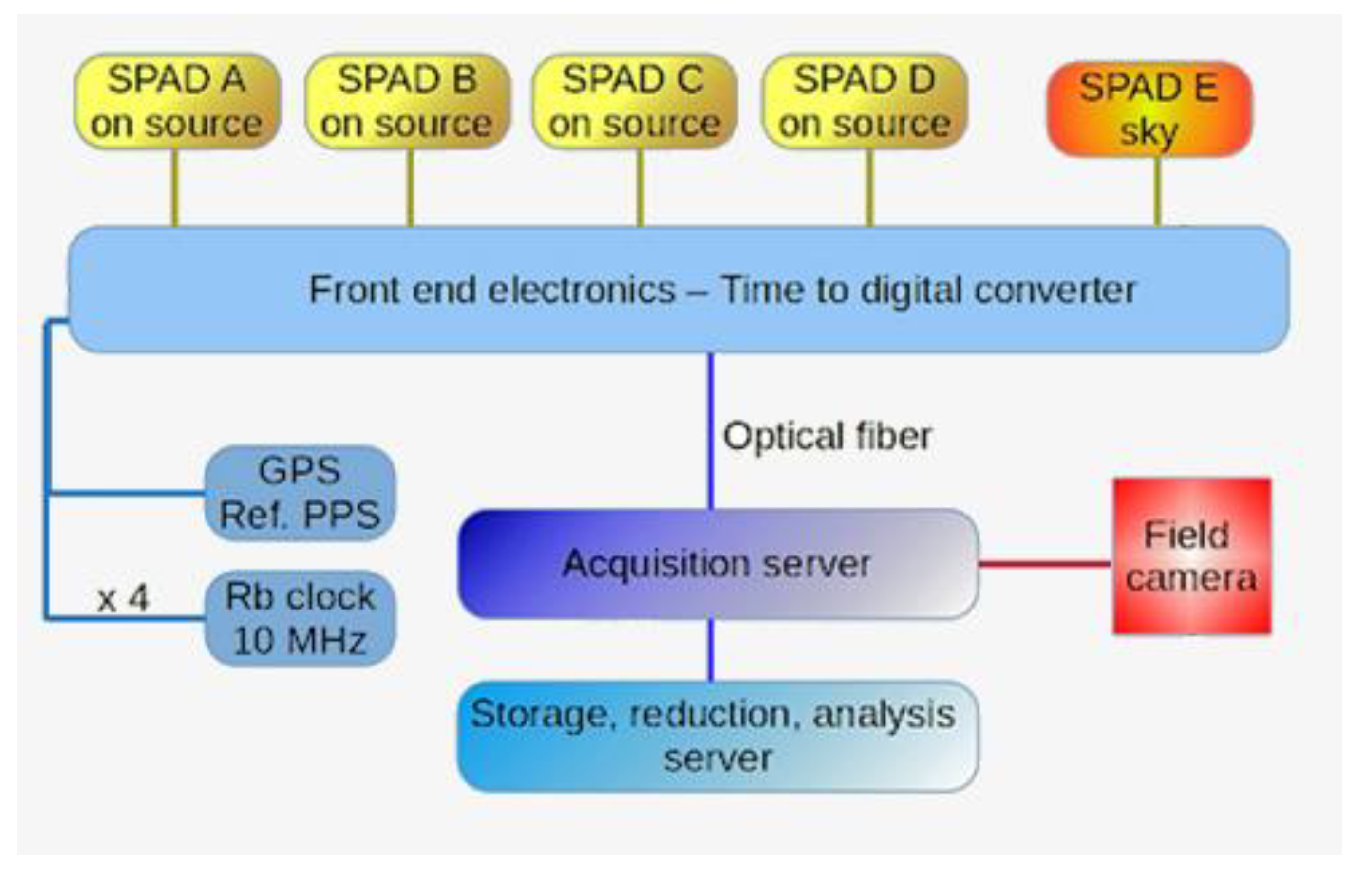
2. From QuantEye to AquEye and IquEye

In QuantEye, we described how to couple the enormous 100 m aperture of OWL to an array of 50 μm diameter ultrafast single photon detectors: this was realized by subdividing the exit pupil of the telescope in 10 × 10 sub-pupils by means of a lenslet array, with each sub-pupil feeding its own detector [2]. To test such a scheme in real telescopes, we took advantage of the availability of our 1.8 m Copernicus telescope at Cima Ekar, Asiago. Given the much smaller dimensions of the telescope with respect to OWL, pupil subdivision was achieved in a much simpler way, by means of a four-face reflecting pyramid [10]. After the pyramid, a relay objective, composed of a two-lens system, focusses the light on the detectors. Filters to select the desired bandwidth can be inserted before the pyramid or even in between the two systems composing the relay objective. With this solution, a single-photon multi-wavelength non-imaging photometer could be built.
Two instruments adopting this optical design were actually built: AquEye (the Asiago Quantum Eye) for the Copernicus telescope, later upgraded to AquEye+, and IquEye (the Italian Quantum Eye), to be mounted on 4 m class telescopes such as the ESO NTT in La Silla (Chile) (Figure 1 shows the two instruments presently in use at the Asiago Observatories). A fifth detector was added to both instruments to monitor the intensity and variations of sky brightness adjacent to the targeted star. The two photometers differ in dimensions and other details, but the basic optical and electronic schemes are identical. Accurate descriptions have been given in [10,11,12], so only basic information is provided here. As shown in Figure 1, AquEye+ continues its work with the Copernicus telescope. IquEye, after several successful runs at the NTT, has been brought back to Asiago and now is operating at the 1.2 m Galileo telescope facility with a fiber-optic feed from its Cassegrain focus [13].
The Single Photon Avalanche Diodes (SPADs) produced by MicroPhotonDevices (MPD) in Italy were chosen as detectors. We used MPD SPADs with sensitive area diameters of either 50 µm or 100 µm; they have 34 ps nominal time resolution when coupled to an NIM connector (34 ps is the half-maximum width of the generated current pulse), quantum efficiency peaking to about 60% in the visual band, integrated thermal control, and a ruggedized casing. A minor drawback is a dead time of about 75 nanoseconds after the arrival of a photon, implying a maximum count rate of 13 MHz with no overlaps of arrival times. The sensitivity of the two photometers, calculated considering the SPADs’ quantum efficiency and the pyramid plus mirrors reflectivity, peaks in the visible range, reaching about 35%. Detailed calculations of IquEye sensitivity at the NTT and exposure times to reach a wanted S/N for stars in different magnitudes, both in visible light and in the BVRI photometric bands, are shown in Figures 4 and 5 of [11]. The linear sensitivity from the 5th to the 17th magnitude, which provides the largest dynamic range of any astronomical photometer, is very noticeable.
To acquire the signals from the five SPADs, a time-to-digital (TDC) unit produced by CAEN in Italy was selected. This unit, with an internal clock ticking every 24 ps, has 16 input channels, five used for the SPADs and two for GPS and Rubidium clock ticks. The output from the TDC is fed into the memory of the computer, recording each individual count. Taking into account the whole chain of electronics from the SPADs to the TDC, we can claim a relative accuracy in the determination of the arrival time of each photon of around 100 ps, and an absolute (with respect to UTC) accuracy of less than 0.5 ns for acquisition times longer than 30 min. Therefore, in the a-posteriori analysis, we can decide the length of the time bins (from 100 ps to any desired upper limit) to maximize the S/N ratio for the scientific goal under consideration. A schematic of the overall system is shown in Figure 2.

3. Astrophysical Results

AquEye+ and Iqueye have been employed for a variety of astrophysical problems. We report here some results for optical pulsar light curves, lunar occultations, and intensity interferometry.

3.1. Optical Pulsar Light Curves

Pulsars (namely pulsating radio stars) are rotating neutron stars with a diameter of around 10 km and a mass of approximately one solar mass. Only a fraction of pulsars show pulsations in bands of the electromagnetic spectrum different from radio, and in particular in the optical band. As the optical radiation from pulsars is generally agreed to come from incoherent synchrotron radiation, a comparison of observations in the visible portion of the spectrum with the radio, UV, X-ray and gamma bands allows one to probe the geometry of the respective emitting regions and of the magnetic field configuration, as well to measure the energy spectrum of the emitting electrons.
Given the excellent time tagging accuracy of AquEye and Iqueye, we observed optical pulsars with both photometers whenever possible. Indeed, we measured the light curves of several optical pulsars, starting with the most observed one, that is, in the Crab Nebula.

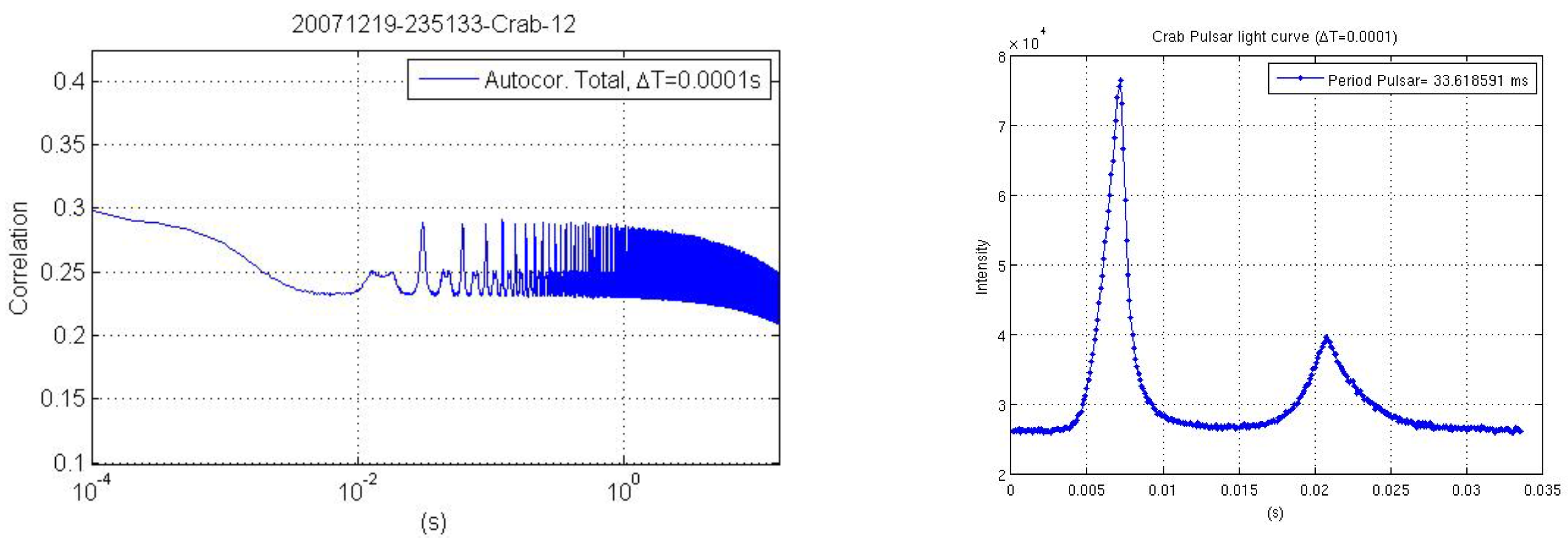
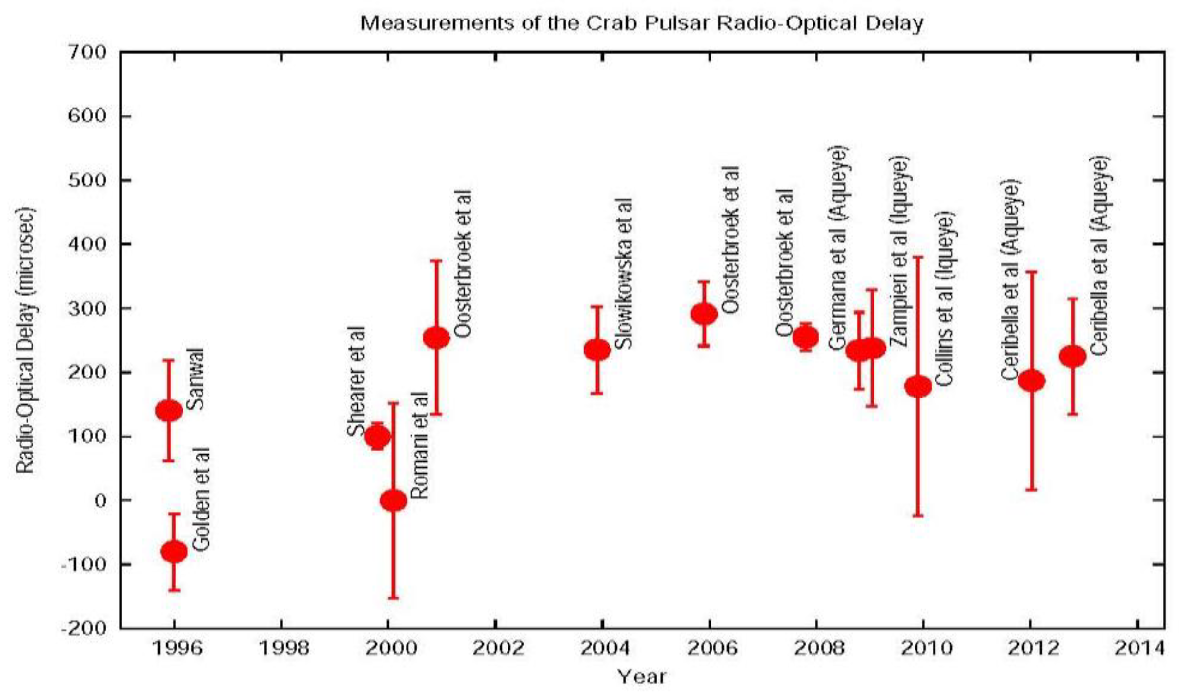
3.1.1. The Crab Nebula Pulsar

The Crab Nebula pulsar (PSR 0531+21) is the brightest optical pulsar, about 2 kpc distant, with an apparent visual magnitude V ≈ 16.6. As is well known, the pulsating star is the remnant of a Type II supernova observed by Chinese astrologers in A.D. 1054. Its favorable position in the sky allows its study from both hemispheres, in our case from Asiago in Italy and La Silla in Chile. Thanks to several observations with these telescopes, and in particular a year-long monitoring from Asiago, we published several papers on the most important timing parameters and characteristics of this interesting pulsar [13,14,15,16,17,18].
Figure 3 shows some observational data obtained with AquEye at the Copernicus facility on 7 December 2007, one of our earliest acquisitions, demonstrating the capabilities of the instrument. The left panel shows the normalized autocorrelation function, the right panel the double peaked light curve, after only 30 s of acquisition and data binned to 0.1 milliseconds. The larger photon flux produced by the 3.6 m NTT in La Silla allowed IquEye to detect in real time each individual double peak.
In parallel with improvements in the hardware and observational procedure, the data analysis procedure was gradually refined, implementing the TEMPO2 package [19,20] for accurate barycentering of the arrival times [17]. Briefly, it was found that over a 1 year time span, a parabolic fit is no longer adequate to model the pulsar spin-down. Therefore, a third-order polynomial fit was adopted to describe the phase behavior, with the expression:
ψ ( t ) = ϕ 0 + ( ν ν int ) ( t t 0 ) + 1 2 ν ˙ ( t t 0 ) 2 + 1 6 ν ¨ ( t t 0 ) 3
where the first and second derivative of the frequency appear together with the initial parameters. Indeed, the quality of the data is such that we can derive the first derivative after a few hours of observations, and the second after a few days. Expression (1) has been further refined with the following considerations: in several spin-down theoretical models, it is stated that the first derivative satisfies the so-called braking index relation:
ν ˙ = K ν n
where K is a constant and n is the braking index; the latter depends on the mechanisms responsible for the loss of angular momentum and of rotational energy of the star. By means of (2), a fourth term was added to (1), giving the expression:
ψ ( t ) = ϕ 0 + ( ν ν int ) ( t t 0 ) + 1 2 ν ˙ ( t t 0 ) 2 + n 6 ( ν ˙ 2 ν ) 0 ( t t 0 ) 3 + n ( 2 n 1 ) 24 ( ν ˙ 3 ν 2 ) 0 ( t t 0 ) 4
Inserting the parameters of the Crab pulsar (namely ν ≈ 30 Hz, ν ˙ 0 ≈ –4 × 10⁻¹⁰ s−2, n ≈ 2.44), we estimated that 2.5 days are needed for a reliable determination of the parabolic term, 6 months for the cubic one and 4 years for the fourth-order term. In turn, a parabolic analysis is sufficient to properly analyze observations spanning a few days, and a cubic expression for several months, while a full fourth-order analysis is required for several years of data. Noticeably, during the period from January to December 2009, when we could observe with IquEye at the NTT facility, the pulsar had so closely followed a braking index law that we were able to count almost nine hundred million turns of the pulsar, with an uncertainty of only two turns.
Fitting the phase law (1) with actual data allowed us to derive a precise estimation of the phase noise. We found that this noise had a Gaussian distribution with a dispersion of about 15 μs in the large majority of the observations, confirming the theoretical expectations for a phase variability induced by photon noise. These data have been used to model the braking mechanism of the pulsar [18]. From the analysis reported in [18], we demonstrated that the pulsar is subjected to jumps in rotational frequency, the so called glitches, which cause abrupt discontinuities in the braking power law. We analyzed 26 years (from May 1988 to June 2015) of data on the Crab pulsar, during which 25 glitches were detected, and we could measure abrupt discontinuous changes in the braking index, whose value varied between ~2.1 to ~2.6, in correspondence with the most intense glitches. The deviations from the regular phase law are very small, as the measured phase residuals have been of no more than 35 turns in more than 2 × 10¹⁰. The analysis we performed on these measurements favors explaining these phase discontinuities as the result of the electromagnetic interactions of the pulsar with the surrounding plasma environment, rather than physical events occurring in the pulsar interior.
Coordinated observations with the Jodrell Bank radio telescope, which daily observes the Crab pulsar and fits the measured data over yearly periods, show agreement in the measurement of instantaneous periods to better than 1 ps, thus confirming the extremely high quality of Aqueye+ and Iqueye data. Moreover, we have confirmed that the sporadic giant radio bursts are accompanied by an increase in the optical flux, see [16].
Another measurement we could perform, thanks to the great absolute time accuracy, was of the delay in the arrival times of the radio vs. optical peaks. Figure 4 shows the measurements of this delay realized from 1966 to 2014 (data from 2006 are from our instruments only). The sign of the delay has reversed since 2000, but one can suspect systematic errors in those early data. Our data confirm that the optical peak precedes the radio peak by about 200 µs.

3.1.2. PSR B0540-69

Another pulsar for which IquEye observations at NTT have provided unique results is the young PSR B0540-69 in the Large Magellanic Cloud, the second brightest pulsar in visible light [29]. The light curve clearly shows that the main peak has a double structure, that the leading edge is steeper than the trailing one, and that there is some residual light in between the main pulses. The measured period varies around 0.0506 s; from its increase over 1 year of observations, we derived a braking index value of n = 2.047 ± 0.050, definitely lower than that of the Crab pulsar. The pulsar age, corrected by the measured braking index, was confirmed to be around 1700 years.
Like both the Crab and Vela (see next paragraph) pulsars, PSR B0540-69 is an isolated pulsar; it has been detected by instruments working in different spectral bands, from radio to near-IR, visible, UV, X-rays, and γ-rays, and it has been seen pulsating in almost all of these energy bands. Our IquEye data could be compared with the UV, X-ray and gamma observations made with the HST, XMM-Newton and Fermi telescopes (see [30,31]): the peaks observed in the optical, X-ray, and γ-ray light curves are synchronous and in phase with those observed in the radio (1.4 GHz); this is a behavior similar to the that observed in the Crab pulsar and demonstrates that the two pulsars have a similar beaming geometry over all of the electromagnetic spectrum.

3.1.3. Vela Pulsar

PSR J0835-4510, namely the Vela pulsar, at a distance of about 300 pc, is one of the most intense sources in the gamma and radio wavebands, and actually it is visible at all energies, including the optical band. Its age of about 11 kyr is intermediate between those of younger optical pulsars such as the Crab and PSR B0540-69 and older systems such as Geminga.
It exhibits a very complex light curve, with at least five different components detected in all energy domains. In the optical region it is very faint, the faintest and slowest we could observe with IquEye, at V = 23.6 and ν ≈ 11.18 Hz (a period P ≈ 0.0894 s). A schematic representation of the optical light curve, based on IquEye data, is given in Figure 5.
A very detailed analysis of this light curve and a comparison with those in the other bands is reported in [32]. Phase fitting was carried out using the same procedure expounded for the Crab pulsar in Equation (1), using an initial period P = 0.08936694 s. The derived spin-down amounts to ν ˙ 0 ≈ −1.36 × 10⁻¹¹ Hz/s, and the measured rotational period agrees (within ≈≈20 ns error) with that derived from the available radio ephemerides. We also compared the more complex visible light curve obtained with IquEye data with that obtained with Fermi-LAT observations in the gamma rays: thanks to the great absolute time accuracy of both instruments, coupled to radio observations, we have been able to measure the relative shift in the time of arrival of the radio, visible and gamma peaks with an accuracy of a fraction of millisecond (see in particular Figures 4 and 5 and Table 5 in [32]). For instance, we found that the gamma peak named P1h precedes the corresponding optical peak P1s by 11.2 ± 0.4 ms (that is a difference of 0.125 ± 0.004 in phase), while the gamma P2h peak trails the corresponding visible double peak P2s by less than 9 ms; also, the P4 peak observed with Iqueye, and not present in the gamma light curve, is aligned in phase with the radio peak within the measurement errors.
Such a detailed comparison showed again the excellent quality of the IquEye data and also highlighted features of the Vela pulsar light curve that had not been identified before, such as, for example, the double-peak structure of peak P2s and the faint peak P3.

3.1.4. PSR J1023+0038

AquEye+ at the Copernicus facility has shown its virtue by observing the transitional pulsar PSR J1023+0038, the fastest optical pulsar we could observe to date, with a period of 1.688 ms ([33,34]). The timing solution we derived in visible light with just a few days of observations has an accuracy of about ∼12 μs, which corresponds to ∼0.007 in phase. After 2 years of data (from 2018 to 2020), we could determine the spin-down rate of the pulsar, which was found to be –2.53 ± 0.04 × 10⁻¹⁵ Hz2. This pulsar, too, is observable in the UV and X-ray bands. As described in [35], (quasi-)simultaneous observations were obtained with AquEye+ and the XMM-Newton and NICER X-ray instruments. These observations, and in particular those acquired with AquEye+ and NICER, pointed out that the optical pulses follow the X-ray pulses by ∼150 μs, with an uncertainty that is much smaller than the measured time shift.
As pointed out earlier, the ability to store each individual data point without any integration allows one to analyze the data with different statistical methods. A method we used from the beginning was the so-called waterfall diagram, shown in Figure 6.
The method has been refined in [36], with a re-examination of the capabilities of principal component analysis (PCA). Figure 2 in [36] shows more in detail how the method works. If the adopted folding period is only slightly different from the correct one, the two lines are appreciably slanted. They appear rigorously vertical only when the period adopted for folding the data corresponds to the actual one.

3.2. Lunar Occultations

Measuring lunar occultations is another successful program involving AquEye+ at the Copernicus telescope and IquEye at the Galileo one. Such programs exploit at their best the unique properties of these photometers, which are the capability of realizing simultaneous measurements with four different filters, by means of the adopted pupil splitting optical configuration, and presently the best instrumental time resolution, which can reach the nanosecond level. The latter enables Aqueye+ and Iqueye to observe not just Moon occultations, but also much faster events, such as occultations by asteroids, by TNOs [37] and even, theoretically, occultations by artificial screens in space.
A detailed account of nine lunar occultations is given in [38]. Recorded photon events were analyzed in post-processing with different time bins and fa model-dependent least square method. Among the results expounded therein, we mention that we could measure the size of the chromosphere of the bright star µ Psc: Figure 7 shows the data taken by AquEye+ during its immersion below the lunar disk. The oscillations of luminosity preceding the immersion of the star under the lunar limb, due to diffraction from the lunar edge, are clearly seen in the shortest time bin (upper panel). The best fit to the data is provided by a model representing a star with a uniformly illuminated disk of 3.14 milliarcseconds in diameter.

3.3. Stellar Intensity Interferometry

Stellar intensity interferometry (SII) is a technique that allows one to obtain spatial (angular) information from the observed stellar target, by measuring the spatial correlation of the star light intensity simultaneously collected by two physically separated telescopes, A and B. This subject is treated in several books and papers; see, for instance, [39,40]. As an example, in the case of chaotic thermal light (i.e., light with a Gaussian amplitude distribution), that is the most common coFndition for stellar objects, this correlation is associated with the mutual degree of coherence between the two positions. Given the time average intensities I A and I B , over a time interval T, of the stellar object intensity at telescopes A and B, respectively, and I A I B the spatial correlation in the same time interval, we obtain for the second order coherence:
g ( 2 ) = I A I B I A I B = 1 + | γ | 2 2
where γ is the (complex) degree of coherence of light; its absolute value provides the visibility function of the fringes in a classical interferometer.
Equation (4) gives the second order coherence function when a continuous intensity signal is detected at the focal planes of the two telescopes. However, this function can be expressed also in a discrete form, that is, when working in photon counting mode, thus having a discontinuous signal, obtaining:
g ( 2 ) = n N A B N A N B   ;
where NA and NB are the number of photons respectively detected at telescopes A and B during the observing interval T, NAB is the number of simultaneous detections (i.e., events observed at both telescopes in the same short time bin dt) in T, and n is the number of observed time bins ( n = T / d t ).
By means of probabilistic analysis and integrating over time T, it can be determined [41], in case of unpolarized light, that the number of coincidences is:
N A B = 1 T N A N B d t + 1 2 γ ( τ ) 2 d τ
finally obtaining that
g ( 2 ) = 1 + 1 2 g ( 0 ) 2 τ c / d t   ;
In this equation, τc = 1/Δν = (λ/c)(λλ) is the coherence time of observed light. Its value is given by the bandwidth Δλ of a narrow band filter used along the optical path and is found as a compromise between the need for a narrow Δλ to obtain a large g(2) value and the need for a reasonably high number of coincidence events that depend on the telescope size and throughput. For example, with few-meter class telescopes in visible light, a typical filter bandwidth is of the order of Δλ = 1 nm, which corresponds to a coherence time of approximately τc = 1 ps.
Analysis also shows that the S/N ratio for g(2) measurements depends on the photon statistics and is equal to
S N = F A α γ 2 T 2 d t .
In this equation, F is the source rate in photons per unit area and time, within an optical bandwidth Δν (in Hz); A is the telescope area, and α is the global quantum efficiency of the detectors. Using wavelength instead of frequency, Equation (8) can be rewritten as:
S N = F λ c λ Δ λ α γ 2 T 2 d t
The relevant observable of this measurement is the |g(0)|2 term in Equation (7), and is obtained from the difference g(2)—1 after having measured g(2) by means of (5). This difference comes from the tiny excess of correlated coincidences, with respect to the large majority of random uncorrelated ones, due to the quantum nature of light. In practice, SII is an inherently inefficient technique that requires the largest possible apertures and the most sensitive, fastest detectors. However, SII has several advantages over phase interferometry:
  • Rather relaxed geometric accuracy, meaning that precisions of centimeters are required for making an intensity interferometry measurement, to be compared with the fraction of wavelength (sub-micron in visible light) needed for realizing classical phase interferometers.
  • For the same reason, there is no need to have telescope mirrors with high optical quality; the actual, most stringent limitation is to minimize the amount of stray light/background on the sensor.
  • Negligible sensitivity to seeing conditions (on timescales as short as fractions of a ns, the atmospheric turbulence is essentially frozen), so that there is no need to use adaptive optics.
  • Correlation is performed at the measured signal level, which can be a current or, as in our case, a string of photon time tags; for this, just an accurate time reference is needed, and there is no need for ad-hoc optical links between telescopes to realize interference between the optical light beam, as with phase interferometers.
Such considerations, coupled to the present and near-future availability of large telescopes, efficient detectors, fast computers and large storage memories, have prompted the resurrection of SII.
The calculation of g(2) in the photon counting regime is not a simple task [42]. We succeeded in carrying out a pioneering experiment using the fiber-fed IquEye at the 1.22 m and AquEye+ at the 1.82 m telescopes in Asiago. The telescopes are separated by about 3.4 km and 300 m in elevation [41,43,44,45]. The measurements were realized through selecting the wavelength band by means of a series of an H-α filter, a ×10 neutral density filter, and a narrow band interferometric filter. With our acquisition systems, we stored all of the detected photon time tags, and we correlated them with a suitable post-processing software correlator. The used time bin was dt = 400 ps. Following the variable hour angle of the star during the observations, which lasted several hours on different nigths, the baseline, i.e., the telescope spatial separation perpendicular to the target line of sight, varied in the range 1535–2418 m, and the detected time tags were corrected for the light travel time delay between the telescopes. Due to the limited size of the Asiago telescopes and their large separation, we could perform just two correlation measurements: one at zero baseline, where we expected to detect a very small signal, and one at ~2 km baseline, where we expected no correlation. Ours (see [45]) is the first-ever post-processing measurement of correlation on an astronomical target, and it has been realized by means of a photon counting software correlator. The average discrete degree of coherence for Vega measured at zero baseline was <g(2)> = 1.0034 ± 0.0008, while no evidence of correlation was found on the 2 km projected baseline [45]. The measurement, consistent with the estimated diameter of Vega of about 0.003 arcseconds, has the potential to place a direct constraint on bright features on the surface of the star as small as 30 micro-arcseconds.

4. Conclusions

AquEye+ and IquEye, which have shown their usefulness on a variety of very-high time-resolution astrophysical problems and even in SII with small telescopes, have been briefly reviewed in this paper. It is worth mentioning that the ideas expounded in QuantEye, and that we proved with our instruments, will come to full fruition with large-aperture telescopes such as ESO’s ELT, now nearing completion. In the near future, arrays of Cherenkov light telescopes also will be used to realize intensity interferometry (like the ASTRI mini-array [46,47,48] being built in Izaña, Tenerife): this will provide unparalleled angular resolutions over several directions in the sky, placing constraints also on bright features on the stellar surface. The sensitivity with such apertures and modern photon counters will allow measurements of the diameters of stars of magnitudes up to 7, as well as the realization of star disk imaging thanks to the many different baselines available.

Author Contributions

Writing—original draft preparation, C.B.; writing—review and editing, C.B., G.N. and L.Z. All authors have read and agreed to the published version of the manuscript.

Funding

This research received no external funding.

Institutional Review Board Statement

Not applicable.

Informed Consent Statement

Not applicable.

Data Availability Statement

Data is available on the AquEye+/IquEye Public Data Archive (link from the AquEye+IquEye web page: https://web.oapd.inaf.it/zampieri/aqueye-iqueye/ accessed on 26 July 2023). Access is granted upon request to: aqueye.iqueye@gmail.com.

Conflicts of Interest

The authors declare no conflict of interest.

References

  1. Barbieri, C.; Da Deppo, V.; D’Onofrio, M.; Dravins, D.; Fornasier, S.; Fosbury, R.; Naletto, G.; Nilsson, R.; Occhipinti, T.; Tamburini, F.; et al. QuantEYE, the quantum optics instrument for OWL. Proc. Int. Astron. Union 2005, 1, 506–507. [Google Scholar] [CrossRef]
  2. Barbieri, C.; Dravins, D.; Occhipinti, T.; Tamburini, F.; Naletto, G.; Da Deppo, V.; Fornasier, S.; D’Onofrio, M.; Fosbury, R.A.E.; Nilsson, R.; et al. Astronomical applications of quantum optics for extremely large telescopes. J. Mod. Opt. 2007, 54, 191–197. [Google Scholar] [CrossRef]
  3. Barbieri, C.; Naletto, G.; Tamburini, F.; Occhipinti, T.; Giro, E.; D’Onofrio, M. From QuantEYE to AquEYE—Instrumentation for Astrophysics on Its Shortest Timescales, High Time Resolution Astrophysics. Phelan, D., Ryan, O., Shearer, A., Eds.; Astrophysics and Space Science Library; Springer: Berlin, Germany, 2008; ISBN 978-1-4020-6517-0. [Google Scholar]
  4. Occhipinti, T.; Zampieri, L.; Naletto, G.; Barbieri, C. Quantum astronomy: Scientific background, technologies, achieved results, and future developments. SPIE Proc. 2018, 10548, 105481K. [Google Scholar] [CrossRef]
  5. Tamburini, F.; Anzolin, G.; Umbriaco, G.; Bianchini, A.; Barbieri, C. Overcoming the Rayleigh Criterion Limit with Optical Vortices. Phys. Rev. Lett. 2006, 97, 163903. [Google Scholar] [CrossRef]
  6. Anzolin, G.; Tamburini, F.; Bianchini, A.; Umbriaco, G.; Barbieri, C. Optical vortices with starlight. Astron. Astrophys. 2008, 488, 1159–1165. [Google Scholar] [CrossRef]
  7. Barbieri, C.; Tamburini, F.; Anzolin, G.; Bianchini, A.; Mari, E.; Sponselli, A.; Umbriaco, G.; Prasciolu, M.; Romanato, F.; Villoresi, P. Light’s Orbital Angular Momentum and Optical Vortices for Astronomical Coronagraphy from Ground and Space Telescopes. Earth Moon Planets 2009, 105, 283–288. [Google Scholar] [CrossRef]
  8. Shen, Y.; Wang, X.; Xie, Z.; Min, C.; Fu, X.; Liu, Q.; Gong, M.; Yuan, X. Optical vortices 30 years on: OAM manipulation from topological charge to multiple singularities. Light. Sci. Appl. 2019, 8, 90. [Google Scholar] [CrossRef]
  9. Hanbury, B.R. The Intensity Interferometer: Its Application to Astronomy; Taylor & Francis: Abingdon, UK, 1974. [Google Scholar]
  10. Barbieri, C.; Naletto, G.; Occhipinti, T.; Facchinetti, C.; Verroi, E.; Giro, E.; Di Paola, A.; Billotta, S.; Zoccarato, P.; Bolli, P.; et al. AquEYE, a single photon counting photometer for astronomy. J. Mod. Opt. 2009, 56, 261–272. [Google Scholar] [CrossRef]
  11. Naletto, G.; Barbieri, C.; Occhipinti, T.; Capraro, I.; Di Paola, A.; Facchinetti, C.; Verroi, E.; Zoccarato, P.; Anzolin, G.; Belluso, M.; et al. Iqueye, a single photon-counting photometer applied to the ESO new technology telescope. Astron. Astrophys. 2009, 508, 531–539. [Google Scholar] [CrossRef]
  12. Zampieri, L.; Naletto, G.; Barbieri, C.; Verroi, E.; Ceribella, G.; D’Alessandro, M.; Farisato, G.; Di Paola, A.; Zoccarato, P. Aqueye+: A new ultrafast single photon counter for optical high time resolution astrophysics. SPIE Proc. 2015, 9504, 95040C. [Google Scholar] [CrossRef]
  13. Zampieri, L.; Naletto, G.; Barbieri, C.; Burtovoi, A.; Fiori, M.; Spolon, A.; Ochner, P.; Lessio, L.; Umbriaco, G.; Barbieri, M. (Very) Fast astronomical photometry for meter-class telescopes. Contrib. Astron. Obs. Skaln. Pleso 2019, 49, 85–96. [Google Scholar]
  14. Zampieri, L.; Germanà, C.; Barbieri, C.; Naletto, G.; Čadež, A.; Capraro, I.; Di Paola, A.; Facchinetti, C.; Occhipinti, T.; Ponikvar, D.; et al. The Crab pulsar seen with AquEYE at Asiago Cima Ekar observatory. Adv. Space Res. 2011, 47, 365–369. [Google Scholar] [CrossRef]
  15. Germanà, C.; Zampieri, L.; Barbieri, C.; Naletto, G.; Čadež, A.; Calvani, M.; Barbieri, M.; Capraro, I.; Di Paola, A.; Facchinetti, C.; et al. Aqueye optical observations of the Crab Nebula pulsar. Astron. Astrophys. 2012, 548, A47. [Google Scholar] [CrossRef]
  16. Collins, S.; Shearer, A.; Stappers, B.; Barbieri, C.; Naletto, G.; Zampieri, L.; Verroi, E.; Gradari, S. Crab Pulsar: Enhanced Optical Emission During Giant Radio Pulses. New Horiz. Time-Domain Astron. Proc. Int. Astron. Union IAU Symp. 2012, 285, 296–298. [Google Scholar] [CrossRef]
  17. Zampieri, L.; Čadež, A.; Barbieri, C.; Naletto, G.; Calvani, M.; Barbieri, M.; Verroi, E.; Zoccarato, P.; Occhipinti, T. Optical phase coherent timing of the Crab nebula pulsar with Iqueye at the ESO New Technology Telescope. Mon. Not. R. Astron. Soc. 2014, 439, 2813–2821. [Google Scholar] [CrossRef]
  18. Čadež, A.; Zampieri, L.; Barbieri, C.; Calvani, M.; Naletto, G.; Barbieri, M.; Ponikvar, D. What brakes the Crab pulsar? Astron. Astrophys. 2016, 587, A99. [Google Scholar] [CrossRef]
  19. Hobbs, G.B.; Edwards, R.T.; Manchester, R.N. TEMPO2, a new pulsar-timing package—I. An overview. MNRAS 2006, 369, 655–672. [Google Scholar] [CrossRef]
  20. Edwards, R.T.; Hobbs, G.B.; Manchester, R.N. TEMPO2, a new pulsar timing package—II. The timing model and precision estimates. MNRAS 2006, 372, 1549–1574. [Google Scholar] [CrossRef]
  21. Sanwal, D. Ph.D. Thesis, University of Texas at Austin, Austin, TX, USA, 1999.
  22. Golden, A.; Shearer, A.; Redfern, R.M.; Beskin, G.M.; Neizvestny, S.I.; Neustroev, V.V.; Plokhotnichenko, V.L.; Cullum, M. High speed phase-resolved 2-d UBV photometry of the Crab pulsar. A&A 2000, 363, 617–628. [Google Scholar] [CrossRef]
  23. Romani, R.W.; Miller, A.J.; Cabrera, B.; Nam, S.W.; Martinis, J.M. Phase-resolved Crab Studies with a Cryogenic Transition-Edge Sensor Spectrophotometer. ApJ 2001, 563, 221–228. [Google Scholar] [CrossRef]
  24. Shearer, A.; Stappers, B.; O’Connor, P.; Golden, A.; Strom, R.; Redfern, M.; Ryan, O. Enhanced Optical Emission During Crab Giant Radio Pulses. Science 2003, 301, 493–495. [Google Scholar] [CrossRef] [PubMed]
  25. Oosterbroek, T.; de Bruijne, J.H.J.; Martin, D.; Verhoeve, P.; Perryman, M.A.C.; Erd, C.; Schulz, R. Absolute timing of the Crab Pulsar at optical wavelengths with superconducting tunneling junctions. A&A 2006, 456, 283–286. [Google Scholar] [CrossRef]
  26. Oosterbroek, T.; Cognard, I.; Golden, A.; Verhoeve, P.; Martin, D.D.E.; Erd, C.; Schulz, R.; Stüwe, J.A.; Stankov, A.; Ho, T. Simultaneous absolute timing of the Crab pulsar at radio and optical wavelengths. A&A 2008, 488, 271–277. [Google Scholar] [CrossRef]
  27. Słowikowska, A.; Kanbach, G.; Kramer, M.; Stefanescu, A. Optical polarization of the Crab pulsar: Precision measurements and comparison to the radio emission. MNRAS 2009, 397, 103–123. [Google Scholar] [CrossRef]
  28. Ceribella, G. Ph.D. Thesis, University of Padova, Padova, Italy, 2015.
  29. Gradari, S.; Barbieri, M.; Barbieri, C.; Naletto, G.; Verroi, E.; Occhipinti, T.; Zoccarato, P.; Germanà, C.; Zampieri, L.; Possenti, A. The optical light curve of the LMC pulsar B0540-69 in 2009. Mon. Not. R. Astron. Soc. 2011, 412, 2689–2694. [Google Scholar] [CrossRef]
  30. Fermi LAT Collaboration; Ackermann, M.; Albert, A.; Baldini, L.; Ballet, J.; Barbiellini, G.; Barbieri, C.; Bastieri, D.; Bellazzini, R.; Bissaldi, E.; et al. An extremely bright gamma-ray pulsar in the Large Magellanic Cloud. Science 2015, 350, 801–805. [Google Scholar] [CrossRef]
  31. Mignani, R.P.; Shearer, A.; De Luca, A.; Marshall, F.E.; Guillemot, L.; Smith, D.A.; Rudak, B.; Zampieri, L.; Barbieri, C.; Naletto, G.; et al. The First Ultraviolet Detection of the Large Magellanic Cloud Pulsar PSR B0540–69 and Its Multi-wavelength Properties. Astrophys. J. 2019, 871, 246. [Google Scholar] [CrossRef]
  32. Spolon, A.; Zampieri, L.; Burtovoi, A.; Naletto, G.; Barbieri, C.; Barbieri, M.; Patruno, A.; Verroi, E. Timing analysis and pulse profile of the Vela pulsar in the optical band from Iqueye observations. Mon. Not. R. Astron. Soc. 2018, 482, 175–183. [Google Scholar] [CrossRef]
  33. Zampieri, L.; Burtovoi, A.; Fiori, M.; Naletto, G.; Spolon, A.; Barbieri, C.; Papitto, A.; Ambrosino, F. Precise optical timing of PSR J1023+0038, the first millisecond pulsar detected with Aqueye+ in Asiago. Mon. Not. R. Astron. Soc. Lett. 2019, 485, L109–L113. [Google Scholar] [CrossRef]
  34. Burtovoi, A.; Zampieri, L.; Fiori, M.; Naletto, G.; Spolon, A.; Barbieri, C.; Papitto, A.; Ambrosino, F. Spin-down rate of the transitional millisecond pulsar PSR J1023+0038 in the optical band with Aqueye+. Mon. Not. R. Astron. Soc. Lett. 2020, 498, L98–L103. [Google Scholar] [CrossRef]
  35. Illiano, G.; Papitto, A.; Ambrosino, F.; Zanon, A.M.; Zelati, F.C.; Stella, L.; Zampieri, L.; Burtovoi, A.; Campana, S.; Casella, P.; et al. Investigating the origin of optical and X-ray pulsations of the transitional millisecond pulsar PSR J1023+0038. Astron. Astrophys. 2023, 669, A26. [Google Scholar] [CrossRef]
  36. Cassanelli, T.; Naletto, G.; Codogno, G.; Barbieri, C.; Verroi, E.; Zampieri, L. New technique for determining a pulsar period: Waterfall principal component analysis. Astron. Astrophys. 2022, 663, A106. [Google Scholar] [CrossRef]
  37. Rommel, F.L.; Braga-Ribas, F.; Desmars, J.; Camargo, J.I.B.; Ortiz, J.L.; Sicardy, B.; Vieira-Martins, R.; Assafin, M.; Santos-Sanz, P.; Duffard, R.; et al. Stellar occultations enable milliarcsecond astrometry for Trans-Neptunian objects and Centaurs. Astron. Astrophys. 2020, 644, A40. [Google Scholar] [CrossRef]
  38. Zampieri, L.; Richichi, A.; Naletto, G.; Barbieri, C.; Burtovoi, A.; Fiori, M.; Glindemann, A.; Umbriaco, G.; Ochner, P.; Dyachenko, V.V.; et al. Lunar Occultations with Aqueye+ and Iqueye. Astron. J. 2019, 158, 176. [Google Scholar] [CrossRef]
  39. Labeyrie, A.; Lipson, S.G.; Nisenson, P. An Introduction to Optical Stellar Interferometry; Cambridge University Press: Cambridge, UK, 2006. [Google Scholar] [CrossRef]
  40. Dravins, D.; LeBohec, S.; Jensen, H.; Nuñez, P.D. Optical intensity interferometry with the Cherenkov Telescope Array. Astropart. Phys. 2013, 43, 331–347. [Google Scholar] [CrossRef]
  41. Naletto, G.; Zampieri, L.; Barbieri, C.; Barbieri, M.; Verroi, E.; Umbriaco, G.; Favazza, P.; Lessio, L.; Farisato, G. A 3.9 km baseline intensity interferometry photon counting experiment. SPIE Proc. 2016, 9980, 44–59. [Google Scholar] [CrossRef]
  42. Capraro, I.; Barbieri, C.; Naletto, G.; Occhipinti, T.; Verroi, E.; Zoccarato, P.; Gradari, S. Quantum astronomy with Iqueye. SPIE Proc. 2010, 7702, 77020M. [Google Scholar] [CrossRef]
  43. Zampieri, L.; Naletto, G.; Barbieri, C.; Barbieri, M.; Verroi, E.; Umbriaco, G.; Favazza, P.; Lessio, L.; Farisato, G. Intensity Interferometry with Aqueye+ and Iqueye in Asiago. SPIE Proc. 2016, 9907, 9907–9922. [Google Scholar] [CrossRef]
  44. Fiori, M.; Barbieri, C.; Zampieri, L.; Naletto, G.; Burtovoi, A. Measurement of the second-order g(2) correlation function of visible light from Vega in photon counting mode. SPIE Proc. 2021, 11835, 118350D. [Google Scholar] [CrossRef]
  45. Zampieri, L.; Naletto, G.; Burtovoi, A.; Fiori, M.; Barbieri, C. Stellar intensity interferometry of Vega in photon counting mode. Mon. Not. R. Astron. Soc. 2021, 506, 1585–1594. [Google Scholar] [CrossRef]
  46. Scuderi, S.; Giuliani, A.; Pareschi, G.; Tosti, G.; Catalano, O.; Amato, E.; Antonelli, L.; Gonzàles, J.B.; Bellassai, G.; Bigongiari, C.; et al. The ASTRI Mini-Array of Cherenkov telescopes at the Observatorio del Teide. J. High Energy Astrophys. 2022, 35, 52–68. [Google Scholar] [CrossRef]
  47. Vercellone, S.; Bigongiari, C.; Burtovoi, A.; Cardillo, M.; Catalano, O.; Franceschini, A.; Lombardi, S.; Nava, L.; Pintore, F.; Stamerra, A.; et al. ASTRI Mini-Array core science at the Observatorio del Teide. J. High Energy Astrophys. 2022, 35, 1–42. [Google Scholar] [CrossRef]
  48. Zampieri, L.; Bonanno, G.; Bruno, P.; Gargano, C.; Lessio, L.; Naletto, G.; Paoletti, L.; Rodeghiero, G.; Romeo, G.; Bulgarelli, A.; et al. A stellar intensity interferometry instrument for the ASTRI Mini-Array telescopes. SPIE Proc. 2022, 12183, 157–170. [Google Scholar] [CrossRef]
Figure 1. (Left): AquEye+ at the Cassegrain focus of the Copernicus telescope. (Right): rear view of IquEye in the control room of the Galileo telescope with the scientific SPADs and the fiber-optic feed.
Astronomy 02 00013 g001
Figure 2. The overall system from the scientific SPADs to the storage unit. In addition to the four scientific SPADs, the GPS unit, the Rubidium clock, the fifth SPAD to monitor the sky background and the field camera for target acquisition are shown.
Astronomy 02 00013 g002
Figure 3. (Left) The autocorrelation function of the Crab Nebula pulsar obtained with AquEye at the Copernicus facility. (Right) The light curve after 30 s integration and counts binned at 0.1 milliseconds.
Astronomy 02 00013 g003
Figure 4. Radio-optical delays of the Crab pulsar ([15,16,17,21,22,23,24,25,26,27,28].
Astronomy 02 00013 g004
Figure 5. The complex light curve of the Vela pulsar.
Astronomy 02 00013 g005
Figure 6. The waterfall method applied to the Crab pulsar light curve using the period of the right panel of Figure 3.
Astronomy 02 00013 g006
Figure 7. Star µ Psc occultation data binned at two different time bins: 2.5 ms (upper panel) and 1 s (lower panel).
Astronomy 02 00013 g007
Disclaimer/Publisher’s Note: The statements, opinions and data contained in all publications are solely those of the individual author(s) and contributor(s) and not of MDPI and/or the editor(s). MDPI and/or the editor(s) disclaim responsibility for any injury to people or property resulting from any ideas, methods, instructions or products referred to in the content.

