Article

Uncertainty Quantification and Simulation of Wind-Tunnel-Informed Stochastic Wind Loads †

by
Thays G. A. Duarte
1,
Srinivasan Arunachalam
2,
Arthriya Subgranon
1,* and
Seymour M. J. Spence
2
1
Department of Civil and Coastal Engineering, University of Florida, Gainesville, FL 32611, USA
2
Department of Civil and Environmental Engineering, University of Michigan, Ann Arbor, MI 48109, USA
*
Author to whom correspondence should be addressed.
This paper is an extended version of our paper published in ICASP 14.
Wind 2023, 3(3), 375-393; https://doi.org/10.3390/wind3030022
Submission received: 19 July 2023 / Revised: 15 August 2023 / Accepted: 4 September 2023 / Published: 13 September 2023
(This article belongs to the Special Issue Wind Loads on Buildings and Structures)

Abstract

:
The simulation of stochastic wind loads is necessary for many applications in wind engineering. The proper-orthogonal-decomposition-(POD)-based spectral representation method is a popular approach used for this purpose, due to its computational efficiency. For general wind directions and building configurations, the data-informed POD-based stochastic model is an alternative that uses wind-tunnel-smoothed auto- and cross-spectral density as input, to calibrate the eigenvalues and eigenvectors of the target load process. Even though this method is straightforward and presents advantages, compared to using empirical target auto- and cross-spectral density, the limitations and errors associated with this model have not been investigated. To this end, an extensive experimental study on a rectangular building model considering multiple wind directions and configurations was conducted, to allow the quantification of uncertainty related to the use of short-duration wind tunnel records for calibration and validation of the data-informed POD-based stochastic model. The results demonstrate that the data-informed model can efficiently simulate stochastic wind loads with negligible model errors, while the errors associated with calibration to short-duration wind tunnel data can be important.

1. Introduction

Simulation of multivariate stochastic wind loads is crucial for the performance assessment of mid- and high-rise structural systems and, ultimately, for obtaining reliable designs. Many simulation approaches have been developed and extensively studied for wind engineering applications, such as the wavelet-based method [1,2], the hybrid discrete Fourier transform (DFT), the digital filtering method [3], the autoregressive moving average (ARMA) method [4], and the spectral representation method (SRM) [5,6]. Among these, the SRM has been widely used for a variety of applications, due to its established theory and relative simplicity [6,7,8,9,10]. The SRM consists of simulating the time histories of stationary Gaussian processes that have second-order properties of the input process [5,6,11]. Central to the SRM is the decomposition of the cross-power spectral density (CPSD) matrix corresponding to the stochastic process, which can be done through Cholesky decomposition or proper orthogonal decomposition (POD). The latter has gained popularity, especially for wind engineering applications, with many studies demonstrating its computational efficiency through mode truncation [8,12,13,14,15,16,17]. However, while mode truncation accelerates the simulation, it can influence the accuracy of the simulated signals if an insufficient number of modes are considered, and it needs to be treated with care [15,18].
The critical aspect of the SRM for simulating wind loads is defining the underlying (target) stochastic process. Analytical formulations of the power spectral density (PSD) and CPSD functions have been largely used to define the target load process and are generally limited to a few wind directions (e.g., along-wind, across-wind) and geometries [9,19,20,21,22,23]. Some recent studies have used measured data as input (sample-based), to calibrate the stochastic process [8,10,16,24,25], which is seen as a straightforward and physically meaningful alternative. The advantage of using experimentally estimated spectral functions as the target, as opposed to analytical PSD/CPSD functions, is the possibility of directly capturing in the simulated samples the complex aerodynamic phenomena seen in the wind tunnel. Thus, a data-informed stochastic simulation method has the potential to be calibrated with any given experimental input function and to generate samples with the desired second-order properties for different building geometries, approaching flows, and surrounding configurations. Regardless of the various advantages of wind-tunnel-informed stochastic simulation models, concerns still exist about the limitations they may impose, due to a lack of experimental validation.
Typically, short-duration records collected in wind tunnel tests, with lengths ranging from 30 s to 1 min, are used to calibrate the stochastic wind load model [16,25]. These records can be obtained by conducting high-frequency forcing balance (HFFB) tests or by conducting synchronous multi-pressure sensing system (SMPSS) tests. The latter is commonly preferred, as it provides a more complete picture of the dynamic wind loads acting on the building surface [26,27,28]. Each short-duration record (observation) is a realization of the underlying stochastic process; therefore, only partial/incomplete information about the probabilistic characteristics of the process is available. Ideally, multiple realizations of a stochastic process need to be obtained to describe the underlying process. However, in practice, just one (or, at most, a handful) short-duration time history is obtained for each wind direction and used as the baseline for design. These short-duration records are generally affected by epistemic uncertainties, i.e., imperfect knowledge (e.g., model defects, human errors, low equipment resolution, sampling errors), and aleatory uncertainties, i.e., inherent randomness (e.g., variability of the wind tunnel records collected for the same experimental setup). As a consequence, the underlying statistical properties of the target process will contain errors that can propagate to the simulation of the wind load and, ultimately, the estimation of structural responses. Although several experimental campaigns have been conducted to study the effects of different conditions on wind loading (e.g., different terrain roughness, surrounding structures, etc.), the errors associated with the estimation of the second-order properties of target stochastic processes using short-duration wind tunnel data have not been investigated thoroughly. If not accounted for, these errors can propagate through the stochastic wind load model and can compromise the assessment of structural responses.
The focus of this study is the quantification of the uncertainty associated with the use of short-duration wind tunnel records (e.g., 32 s) to calibrate wind-tunnel-informed POD-based stochastic wind load models for the simulation of wind load time series. An additional discussion on the limitations of the data-informed stochastic wind load model, given input data from different testing conditions, is also provided. To this end, an extensive wind tunnel experimental campaign was conducted on a rectangular building model, considering a total of 19 test conditions involving varying wind directions and experimental setups. The extent of the errors in the simulation model due to the inevitable variability of short-duration records is quantified, as is the efficiency and accuracy of the wind-tunnel-informed POD-based wind load model, in light of model errors and mode truncation.
This study is organized as follows: the background theory on the simulation of multivariate stochastic wind loads through the POD-based SRM is briefly described, followed by a discussion on the wind-tunnel-informed POD-based SRM model; next, the measures adopted to quantify the uncertainties from the use of short-duration wind tunnel records for calibration of the simulation model are presented; subsequently, the wind tunnel experimental testing is described; finally, the results and conclusions are presented.

2. Theoretical Background

2.1. Simulation of Multivariate Stochastic Wind Loads

Wind loads are spatio-temporally varying random processes that can be modeled as stationary in time for a large number of applications. Based on this assumption, let P ( t ; β ) = [ P 1 ( t ; β ) , P 2 ( t ; β ) , , P N ( t ; β ) ] T be considered as the zero-mean fluctuating part of the multivariate stationary wind load process for a given wind direction, β , where N is the total number of wind load components (i.e., the loads or force coefficients associated with each floor level and force direction). According to the POD-based SRM theory [15], the simulation of stationary zero-mean multicorrelated vector-value subprocesses P ˜ i ( t ; β ) can be generated by:
P ˜ i ( t ; β ) = k = 0 N l 1 2 | Ψ i ( ω k ; β ) | Λ i ( ω k ; β ) Δ ω cos ( ω k t + ϑ i ( ω k ) + θ i k )
where Λ i and Ψ i are the ith frequency-dependent eigenvalue and eigenvector of the CPSD matrix of P ( t ; β ) , respectively, N l is the total number of discrete frequencies up to the Nyquist cutoff frequency, Δ ω is the frequency increment with ω k = k Δ ω , θ i k is a uniformly distributed independent random variable over [0, 2 π ] characterizing the stochasticity of the process, and ϑ i ( ω k ) is the phase angle, defined as:
ϑ i ( ω k ) = tan 1 Im ( Ψ i ( ω k ; β ) ) Re ( Ψ i ( ω k ; β ) )
The eigenvalues and eigenvectors, Λ i and Ψ i , can be obtained through the decomposition of the CPSD matrix of P ( t ; β ) , in terms of orthogonal mode functions, by solving the following eigenproblem:
S P ( ω ; β ) Λ i ( ω ; β ) I Ψ i ( ω ; β ) = 0
where S P is the two-sided CPSD matrix of the zero-mean process P ( t ; β ) , which is a Hermitian and non-negative definite [11], and I is the identity matrix. Once the eigenvalues and eigenvectors are obtained, the CPSD matrix of P ( t ; β ) can be expressed by the summation of the contributing modes as:
S P ( ω ; β ) = i = 1 N Λ i ( ω ; β ) Ψ i ( ω ; β ) Ψ i * ( ω ; β )
For many problems in wind engineering, the first few eigenmodes associated with the highest eigenvalues carry the majority of the energy of the process. The truncation of the higher modes enables the following reduced-order modeling of the resultant Gaussian wind load process P G P ( t ; β ) :
P G P ( t ; β ) P ^ G P ( t ; β ) = P ¯ ( β ) + i = 1 N m P ˜ i ( t ; β )
where P ^ G P ( t ; β ) is the truncated representation of P G P ( t ; β ) , P ¯ ( β ) is the mean wind load for a given wind direction β , and N m is the number of contributing modes, such that N m N [15].
While wind pressures are known to have non-Gaussian features, the wind loads may be modeled as a Gaussian process based on the Central Limit Theorem [29]. Therefore, knowledge of second-order statistics is assumed adequate for describing the stochastic wind load process, P ( t ; β ) .

2.2. Wind-Tunnel-Informed POD-Based SRM

The wind-tunnel-informed POD-based SRM is based on the method described in Section 2.1. The basic idea is to calibrate the model to a two-sided CPSD matrix, S P ( ω ; β ) , derived from a typical single short-duration (30 s to 1 min) wind tunnel record [16,25].
To describe the method for the simulation of wind loads, assume P w t ( t ; β ) = [ P w t , 1 ( t ; β ) , P w t , 2 ( t ; β ) , , P w t , N ( t ; β ) ] T , where N is the total number of force components obtained from wind tunnel experimentation and represents the forces F x ( t ) , F y ( t ) , and T z ( t ) acting at the centroid of each floor of the building. To obtain the eigenvalues and eigenvectors of the CPSD matrix of P w t ( t ; β ) and to calibrate the simulation model as in Equation (1), the data-informed smoothed CPSD matrix of the single record needs to be estimated. Welch’s averaging method can be used to this end, which consists of breaking the filtered zero-mean time series P w t ( t ; β ) into K windowed segments of the same length and averaging their periodograms [30,31]. This method reduces the variance of the PSD/CPSD functions, by eliminating noise (random effects), hence facilitating the identification of important patterns and trends in the frequency domain that better align with the underlying PSD/CPSD functions of the process. The smoothed PSD/CPSD functions are then decomposed, using the spectral POD method, to obtain the eigenvalues and eigenvectors, as in Equation (3). The simulation model can be further enhanced through standardization of the input wind tunnel loads or force coefficient time series prior to applying the spectral POD method (see Appendix A). This leads to a more even distribution of energy within the POD, and a lower number of modes is needed to accurately represent the component time series.
This data-informed approach has the key property of incorporating any building-specific aerodynamic phenomena captured in the wind tunnel into the simulation (e.g., vortex shedding and separated flow). Additionally, it enables the simulation of correlated load components acting in the x and y translational directions and the torque around vertical z direction, without the need for a large set of repeated measurements or the development of complex equations to describe the stochastic process for each wind direction and building geometry. However, the estimation of the target matrix, S P ( ω ; β ) , from one short-duration record could potentially lead to significant deviation from the underlying process. It is therefore crucial to quantify the uncertainty related to the use of a single short-duration record for calibrating the simulation model.

3. Uncertainty Quantification

3.1. Errors Induced by Wind Tunnel Data

The main uncertainty investigated in this study is associated with the variability of individual wind tunnel records that are used to calibrate the wind-tunnel-informed POD-based SRM. In this study, the second-order statistics of the processes, such as variance and correlation coefficients, were used to define the uncertainty measures. The target CPSD functions, hereafter referred to as target spectra, were obtained through the ensemble average of multiple wind tunnel records, as described in detail in Section 4, and were used in this study as the baseline for comparison.
The error in the variance can be defined as follows:
ε i ( % ) = σ i 2 σ i T 2 σ i T 2 × 100
where σ i T 2 is the variance associated with the target PSD function, which is estimated in terms of the integration of the PSD functions, and σ i 2 is the variance derived from the integration of the smoothed PSD function, estimated from a single short-duration record. Note that this measure determines the percentage difference between the diagonal terms of the CPSD matrices.
For the off-diagonal terms of the CPSD matrices, percentage error estimates can become meaningless for scarcely correlated signal pairs. Indeed, the target covariance, σ i j T , which is estimated by integrating the co-spectrum (real part of the target CPSD matrix), can have values close to zero for signals with weak correlation. This can lead to large relative errors when σ i j T is used as the denominator in the percentage error estimation. Therefore, errors of the off-diagonal terms in the CPSD functions are assessed by calculating the difference between the correlation coefficients of the target spectra and the correlation coefficients of each smoothed spectra from short-duration records. The error in the correlation coefficients, φ i j , is therefore expressed as:
φ i j = ρ t , i j ρ r , i j
ρ t , i j = σ i j T σ i i T 2 σ j j T 2
ρ r , i j = σ i j r σ i i r 2 σ j j r 2
where ρ t , i j is the correlation coefficient of the target spectra, ρ r , i j is the correlation coefficient associated with individual smoothed spectra estimated from short-duration records, and r = 1 , , R , with R being the total number of wind tunnel records. As correlation coefficients have values ranging from −1 to 1, it is a straightforward measure to judge/interpret the significance of any observed differences.

3.2. Errors Induced by the Model

Previous studies have extensively demonstrated the accuracy and efficiency of the POD-based SRM for generating realizations that match prescribed CPSD functions [15,32]. For validation purposes, the model errors associated with the wind-tunnel-informed stochastic wind load model calibrated to the target spectra were estimated for different experimental conditions. The model errors were computed using the same error measures described in Equations (6) and (7), with the caveat that the smoothed spectra were substituted by the ensemble spectra of the simulated signals, considering all modes.
Additionally, to provide guidance on the selection of a sufficient number of modes for an accurate reduced-order representation of the simulated signals, the error considering higher-order mode truncation was quantified. The effects of wind direction and experimental setup on the truncation error were evaluated. In evaluating the error measures of Equations (6) and (7), the target spectra were used to calibrate the model, while the ensemble spectra of the reduced-order signals were used to characterize the performance of the reduced model.

4. Wind Tunnel Tests

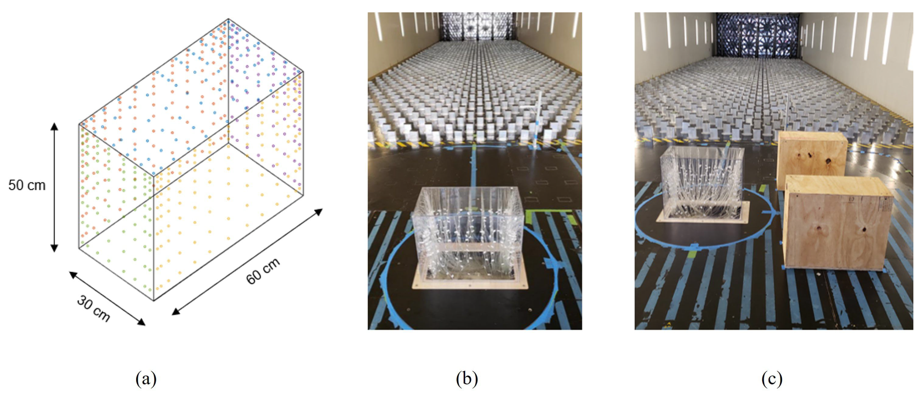
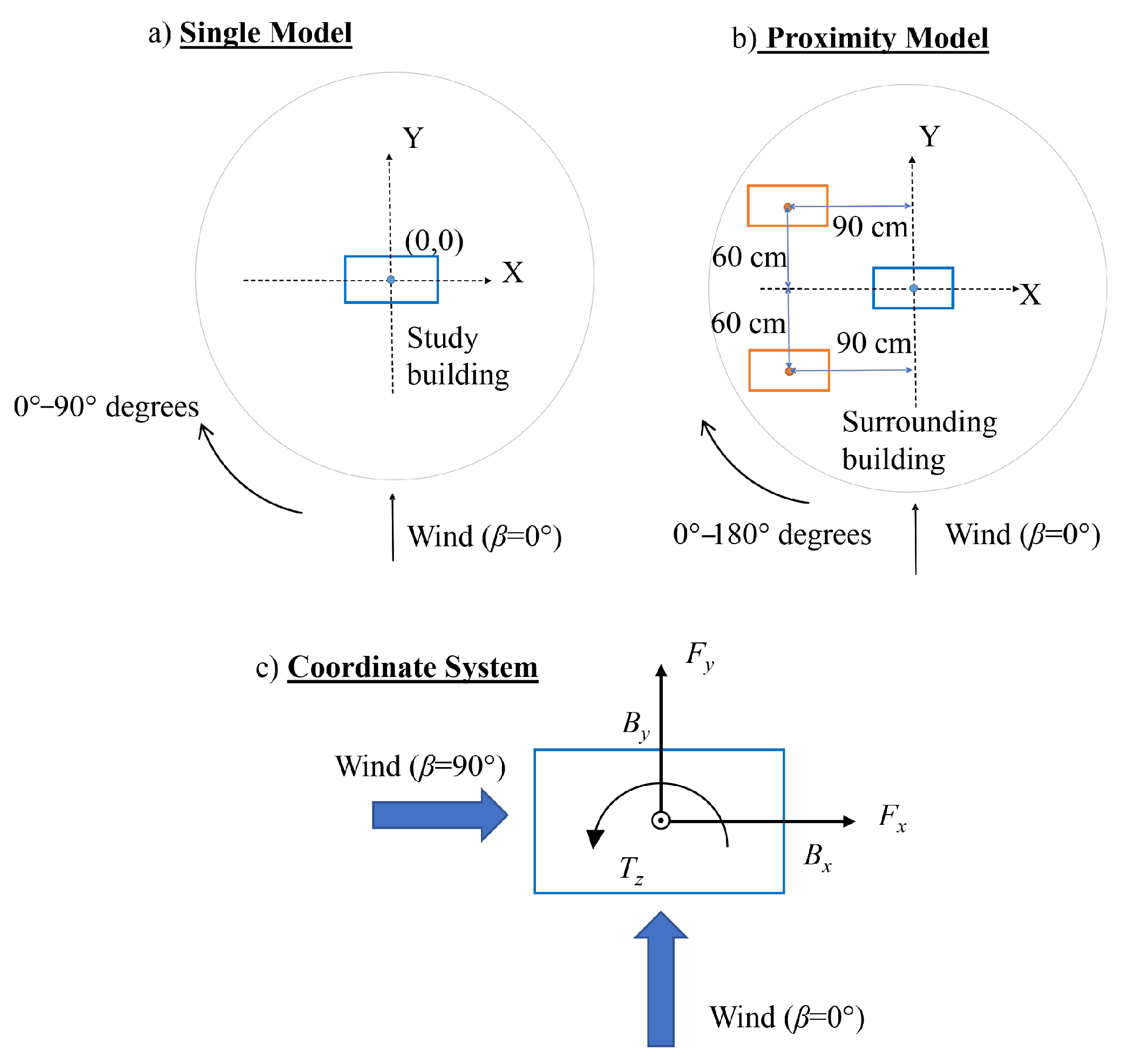
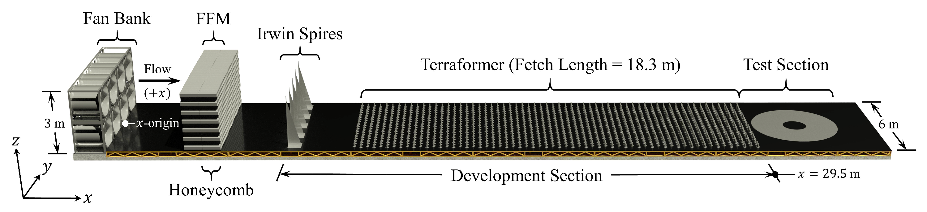
4.1. Experimental Setup

Extensive experimental testing was carried out at the wind tunnel to enable the quantification of the uncertainty associated with individual wind tunnel records. In particular, a rectangular rigid model with geometry and pressure tap distribution shown in Figure 1a was considered. Pressure measurements were simultaneously collected, using a Scanivalve system at 625 Hz sampling frequency. A total of 512 pressure taps were distributed on five surfaces, to capture the flow around the corners and flow variation with height, width, and depth. In this study, only the lateral surfaces were considered, to obtain the resultant forces, as the roof pressures did not contribute to the lateral forces. In total, 19 different testing conditions were conducted for various wind directions and experimental setups. To investigate possible interference effects on the uncertainties of short-duration records, two different testing configurations were considered: the first considered a single model (SM), while the other configuration added two proximity models (PM) with the same geometry as the building model, as shown in Figure 1b,c. For the SM setup, the experiment was conducted for approximately 15 min in model scale and was repeated five times for wind directions varying from 0 to 90 degrees, in increments of 10 degrees, as shown in Figure 2a. Due to the bilateral symmetry of the proximity model test setup, as shown in Figure 2b, five repetitions of 15 min in model scale were carried out, rotating from 0 to 180 degrees, also in 10-degree increments.
The experiments were carried out at the Natural Hazards Engineering Research Infrastructure (NHERI) Boundary Layer Wind Tunnel of the University of Florida. The tunnel is 6 m wide, 3 m tall, and 40 m long, as shown in Figure 3, where the “terraformers” are automated terrain roughness elements with an adjustable height that can be quickly adjusted by electric actuators [33]. For the conducted tests, the height of the terraformer elements was set to 16 cm, in order to obtain a suburban terrain condition. The model scale considered in this study was 1:200, representing a 25-story full-scale building, while the velocity scale was 1:3, leading to a time scale of 1:66.
The external pressure coefficients, C p , e , at each tap location and time, t, were estimated as:
C p , e ( t ) = p ( t ) p 0 q
where p ( t ) was the raw pressure measured at each pressure tap, p 0 was the mean reference static pressure measured by a Cobra Probe located upwind and at the height of the model, and q was the dynamic pressure, defined as q = 1 / 2 ρ U H 2 , with ρ being the local air density, and U H being the mean streamwise wind speed at the model height. Information on the local atmospheric pressure and temperature was used to estimate the air density during the experiments.
The local wind forces acting on the nth floor in the x and y translational directions and the torque around the vertical z direction were obtained by first considering a linear interpolation between the pressure taps, to obtain the pressures acting at each floor level. Then, the pressures were integrated over the tributary area corresponding to the nth floor, to obtain the wind force components. The resultant local forces and moment can be decomposed into F x , n ( t ) , F y , n ( t ) , and T z , n ( t ) components, where n denotes the floor number. Figure 2c shows the forces, coordinate system, and wind directions. The force components at each floor are normalized, to obtain force coefficients as follows:
C F x , n ( t ) = F x , n ( t ) q B x H
C F y , n ( t ) = F y , n ( t ) q B y H
C T z , n ( t ) = T z , n ( t ) q H B max 2 2
where C F x , n ( t ) , C F y , n ( t ) , C T z , n ( t ) are the dynamic force coefficients at the nth floor, H is the height of the model, B x and B y are the plan dimensions of the building, and B max is the maximum plan dimension of the building.

4.2. Processing of the Wind Tunnel Data

In order to evaluate the uncertainties associated with using short-duration wind tunnel records to calibrate the data-informed stochastic model, as defined in Section 3, the wind tunnel data set was divided into two groups: the first group was used to define the baseline target spectra, and the second group—also referred to as the testing set—was used to obtain the smoothed spectra of individual short-duration records. The purpose of dividing the data into two different groups was to obtain unbiased and meaningful error estimates, as the testing set was independent of the data set used to define the target spectra.
The target spectra were obtained using an ensemble average of 750 spectra, estimated using a rectangular window of 4-s duration. Each 4-s record was obtained from non-overlapping intervals extracted from the first 10 min of each wind tunnel test repetition, as described in Section 2.2. In particular, each 10 min set was divided into 150 segments of 4-s duration, while a rectangular window of the same length as the signal was used to ensure zero padding and zero overlapping between the segments. The window size of 4 s was adopted because it was small enough to obtain multiple periodograms to be averaged, as well as to capture the low-frequency content sufficiently well without any padding-based interpolation. A total of 750 segments were used to establish the target spectra for each force coefficient. Ultimately, the target spectra were estimated for all 75 force components for every wind direction and setting.
The remaining 5 min of data were used as a testing set, in order to evaluate the uncertainties as described in Section 3. The testing data were divided into 32-s segments, which were treated as independent short-duration wind tunnel records. The spectra of each short-duration record were obtained, such that the frequency intervals were identical to the target spectra, therefore ensuring the absence of interpolation errors (e.g., zero padding). In particular, Welch’s averaging method was considered, using a Hanning window function of the same length as the target spectra window size, and an overlap of 50%. In general, a total of 45 short-duration records were obtained for each wind direction, with a few directions having fewer records (e.g., 35–44 segments), due to missing data or evident errors in the data set (e.g., abnormal peak pressure values that were up to 50 times larger than the maximum peaks of the entire signal), which were disregarded. Similarly, one of the 4-s segments was disregarded, due to the occurrence of abnormal peak pressure.
A second-order Butterworth lowpass filter with a cutoff frequency of 50 Hz was applied to the dataset, as frequencies only up to a certain value are of interest for practical wind engineering applications. The cutoff frequency was determined, such that unrealistic high-frequency noise caused by equipment was eliminated.

5. Results

5.1. Preamble

The experimental data are employed to estimate the uncertainties associated with the calibration of the wind-tunnel-informed stochastic wind load model using short-duration records (e.g., 32 s). Subsequently, to investigate the effectiveness of the simulation scheme, the model errors and truncation errors are discussed.

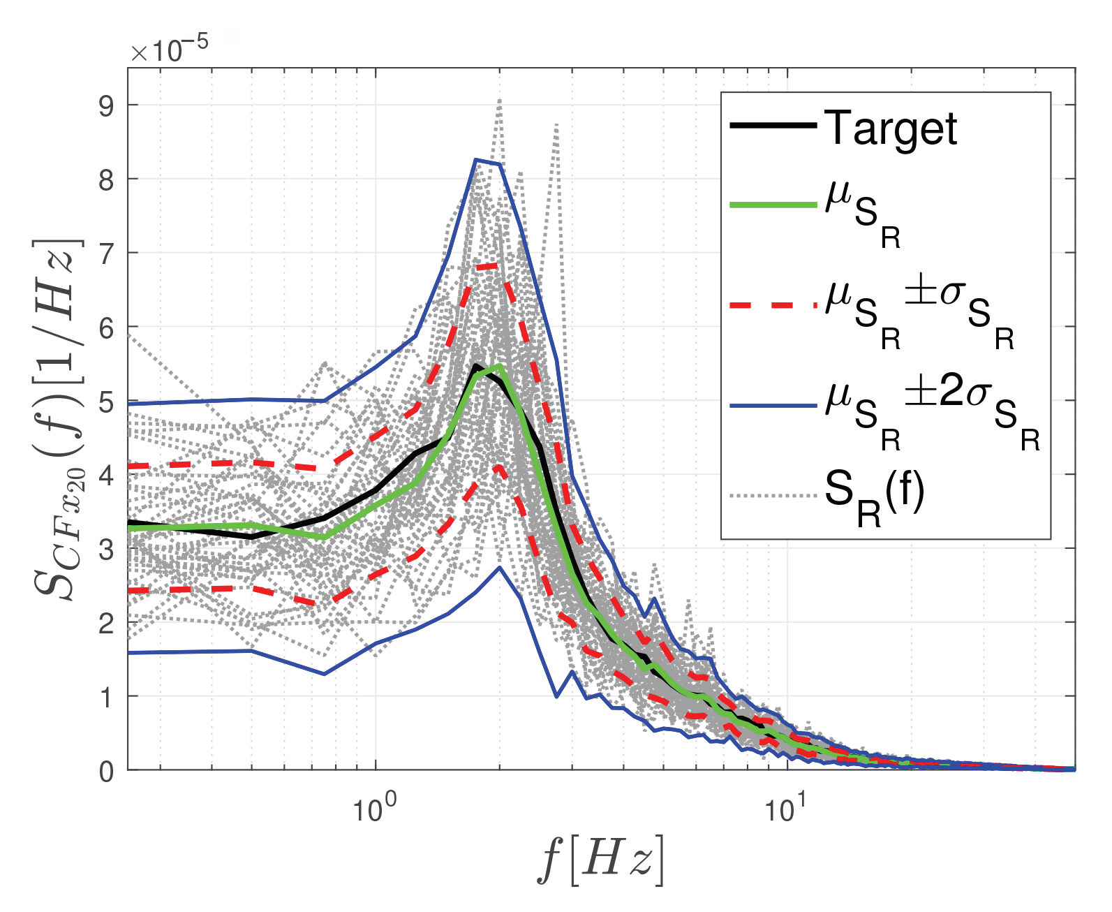
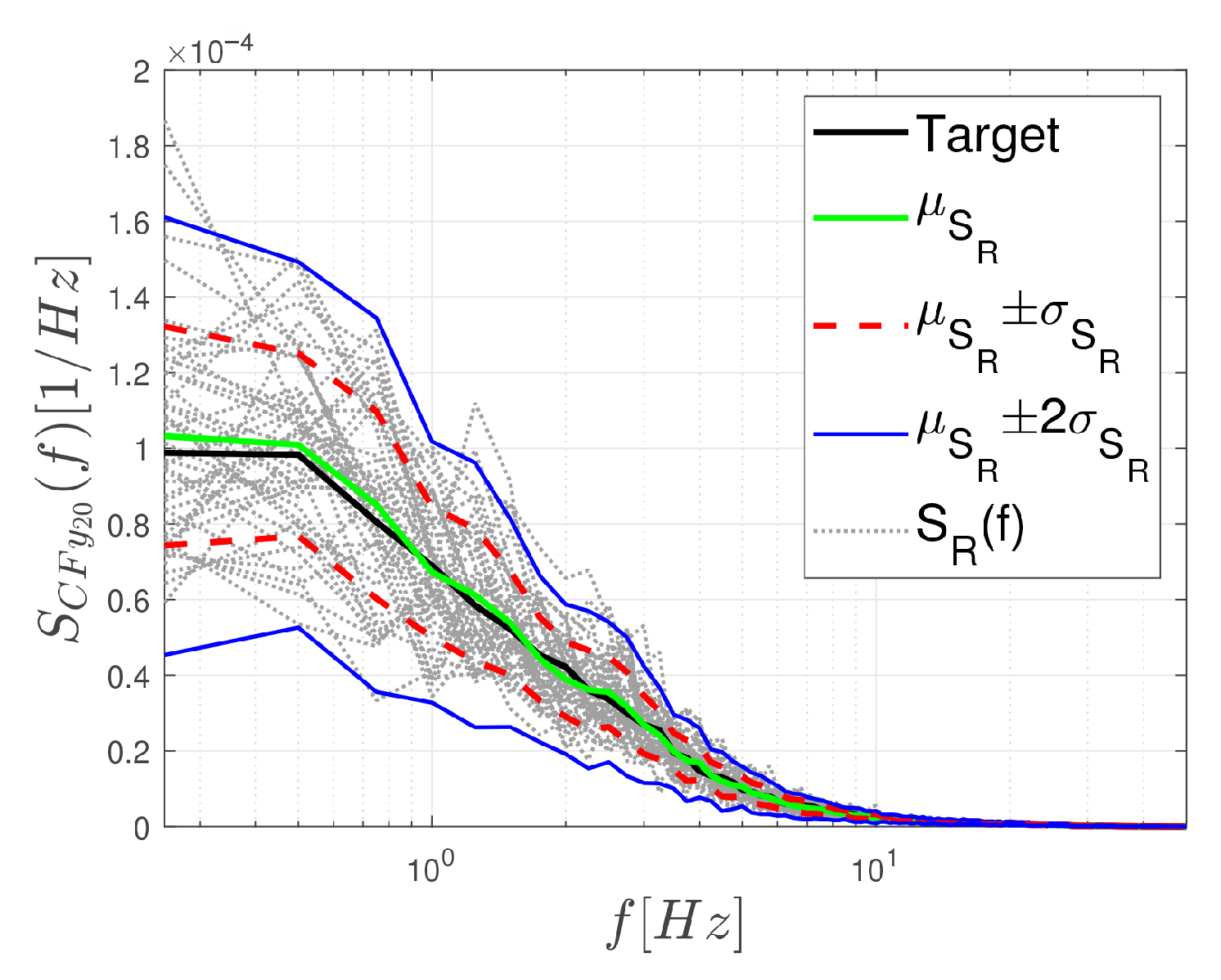
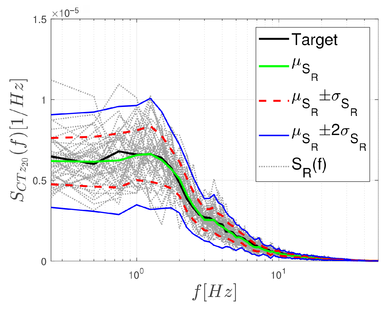
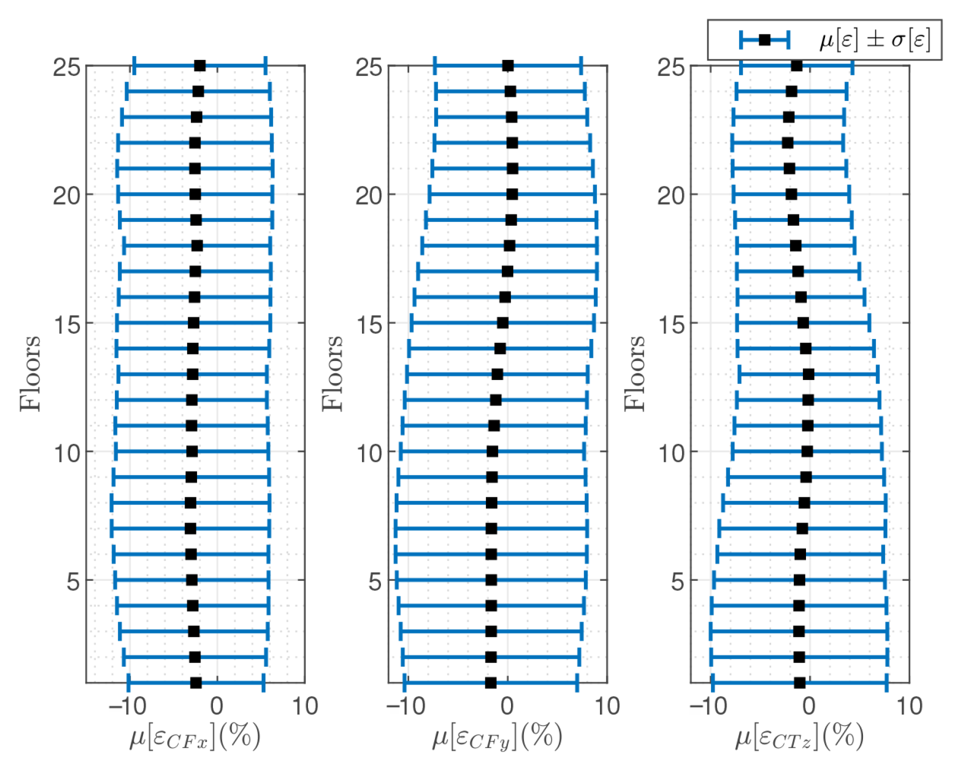
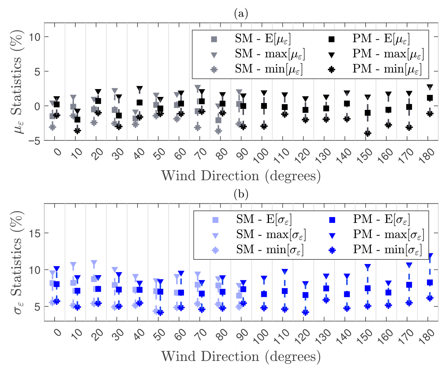
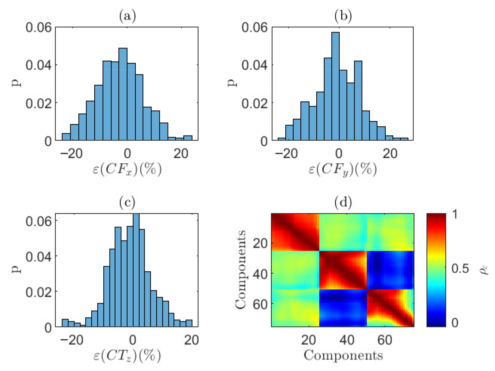
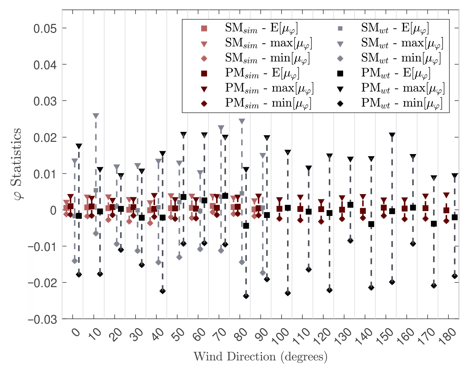
5.2. Errors Induced by the Variability of Short-Duration Wind Tunnel Records

Figure 4, Figure 5 and Figure 6 provide a comparison between the target PSDs (black solid lines)—estimated as in Section 4.2—and the smoothed PSDs (gray dotted lines) of approximately 45 individual realizations of short-duration force coefficient records, S R , at the 20th floor, i.e., C F x , 20 ( t ) , C F y , 20 ( t ) , and C T z , 20 ( t ) , respectively. As can be observed, the smoothed PSDs fluctuate around the target spectra, especially in the lower-frequency region, showing a record variability of up to two standard deviations from the mean. It is also possible to observe that the mean spectra, μ S R , which is obtained from the ensemble average of short-duration records, closely follow the target spectra for the x and y directions, as well as rotations around the vertical z direction. The fact that both curves are visibly close to one another indicates that the individual records are indeed realizations of the target stochastic process, and even though smoothing is applied, considerable variability in the records is clearly evident. The similarity between both curves also indicates the quality and repeatability of the experiment. A similar conclusion could be drawn for all the other floors.
With respect to quantitative measures, the errors in the variance and the errors in the correlation coefficients were estimated as detailed in Section 3. Figure 7 presents the mean, μ ε , and standard deviation, σ ε , of the error in the variance for all force components at each floor and the SM layout for wind direction β = 0 .
In particular, μ ε represents the error between the variance estimated from the target spectra (black solid curve in Figure 4, Figure 5 and Figure 6) and the variance estimated from the mean spectra (green solid line in Figure 4, Figure 5 and Figure 6), whereas σ ε quantifies the spread that individual records can cause on the estimated variances. Overall, it is evident that μ ε ranged between −3% to 0.5% for all force components and all floors, while σ ε varied between 5.5% to 9.6% for this particular wind direction and configuration.
To summarize the ranges of the error measures μ ε and σ ε for all wind directions and both experimental configurations (i.e., SM and PM), Figure 8 presents the expectation, maximum, and minimum values of μ ε and σ ε for all wind directions and both experimental configurations. It is possible to observe from Figure 8 that, overall, both μ ε and σ ε were relatively consistent for all 19 cases studied, with no particular sensitivity to wind direction or testing condition.
In particular, σ ε ranged from about 5% to almost 12%, with an average of around 7.5%. This demonstrates that the smoothed spectra of short-duration records can considerably deviate from the target spectra, regardless of force component and testing condition. Therefore, even though smoothing is applied to reduce noise, the use of short-duration records to calibrate the wind-tunnel-informed stochastic wind load model can introduce significant errors in the simulation. It should be noted that, in general, there are other possible sources of errors: for example, errors generated by experimental setup or those introduced by the integration of pressures over the tributary areas and interpolation to each structural model level. These errors should, in general, be added to the errors discussed in this study. It should be observed that, because a consistent pressure integration method and experimental set were used in this work, such additional errors did not affect the presented results.
To assess the errors in terms of the off-diagonal components of the CPSD matrices, the errors in the correlation coefficients were estimated, using Equation (7). The map of correlation coefficients estimated from the target spectra are presented in Figure 9 for β = 0 and the SM setup. It should be noted that components 1–25, 26–50, and 51–75 refer to the components C F x ( t ) , C F y ( t ) , and C T z ( t ) , respectively.
The map of the mean errors in the correlation coefficients between the target spectra and the smoothed spectra, μ φ , considering all the force components, the SM setup, and β = 0 , is presented in Figure 10. The values of μ φ ranged from around −0.014 to 0.014, which was relatively small compared to the magnitude of the target correlation coefficients in Figure 9, indicating the validity of spectral smoothing in a mean sense. Figure 11 shows the map of the standard deviation, σ φ , of the errors in the correlation coefficients for β = 0 and the SM configuration. It can be observed that highly correlated components showed a smaller σ φ , while higher values were obtained for pairs with a small correlation coefficient. The values of σ φ reached as high as 0.056, indicating uncertainty in the estimation of the correlation coefficients, which agrees with the results presented for the errors in the variance.
To summarize the errors presented in Figure 10 and Figure 11 for all 19 testing conditions, Figure 12 reports the maximum, minimum, and expected values of μ φ and σ φ for all correlation pairs of each wind direction and experimental configuration. It can be seen that E [ μ φ ] , over all floors and force components, fluctuated around zero, indicating that, on average, the correlation structure estimated from the smoothed spectra was close to the target. However, for the standard deviation, the values of σ φ fluctuated around 0.04, with a maximum that could reach as high as 0.08, indicating an important level of variability in the correlation structure estimated from a single short-duration wind tunnel record. Similar to what was seen for the variance, it is also possible to observe that there was no particular sensitivity of the results to the wind direction or testing configuration.
Figure 13a–c presents the histograms of the error in the variance, ε , from all realizations in the testing set for the SM layout and β = 0 . It is possible to observe that the histograms resemble approximately normal distributions, with errors induced from the use of an individual record reaching as high as 20%. Another important finding is presented in the map of Figure 13d, which shows the correlation of the error in the variance ρ ε associated with each force component. It can be observed that there was a high correlation in ε between components acting in the same direction, but a moderate-to low-correlation for components acting in different directions. A similar trend can be observed for other wind directions and settings, in terms of the magnitude of errors, the shape of the histograms, and the correlation of the errors. This, again, indicates the importance of modeling the uncertainty associated with spectral functions estimated from short-duration records.

5.3. Model and Truncation Errors
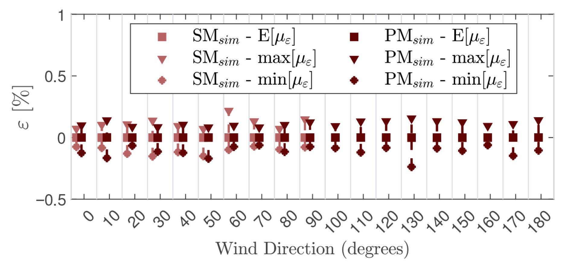
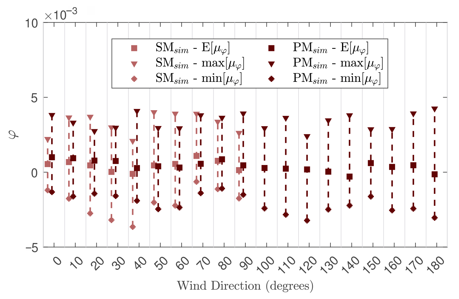
5.3.1. Model Errors

To evaluate the errors associated with the wind-tunnel-informed stochastic wind load model, a set of 40,000 realizations was generated, using the target spectra to calibrate the model. Figure 14 and Figure 15 report the statistics of the errors in the variance and the errors in the correlation coefficients for the 40,000 realizations. It can be seen that for all wind directions and settings, the expected mean error in the variance, E [ μ ε ] , is in the order of 10 4 %, and the expected error in the correlation coefficients, E [ μ φ ] is nearly 0. This demonstrates that the data-driven POD-based stochastic wind load model operates with negligible model error. This agrees with the theory of POD-based SRM models, as the simulation algorithm depends only on the target spectra provided as input, regardless of testing conditions when all modes are considered [17,18,34].
Figure 16 and Figure 17 examine the relative magnitude of the errors that can arise from the stochastic wind load model based on the target spectra, compared to the errors induced by the use of smoothed spectra estimated from a single short-duration record. From these figures, it is evident that model errors are insignificant, compared to the errors introduced by the use of short-duration wind tunnel records when all modes are considered.

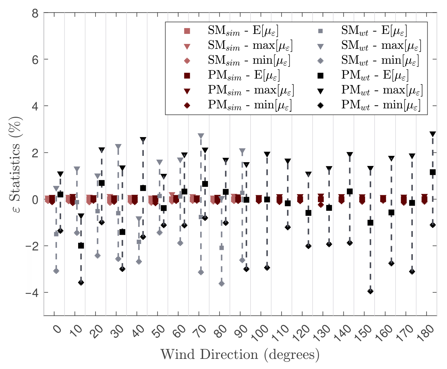
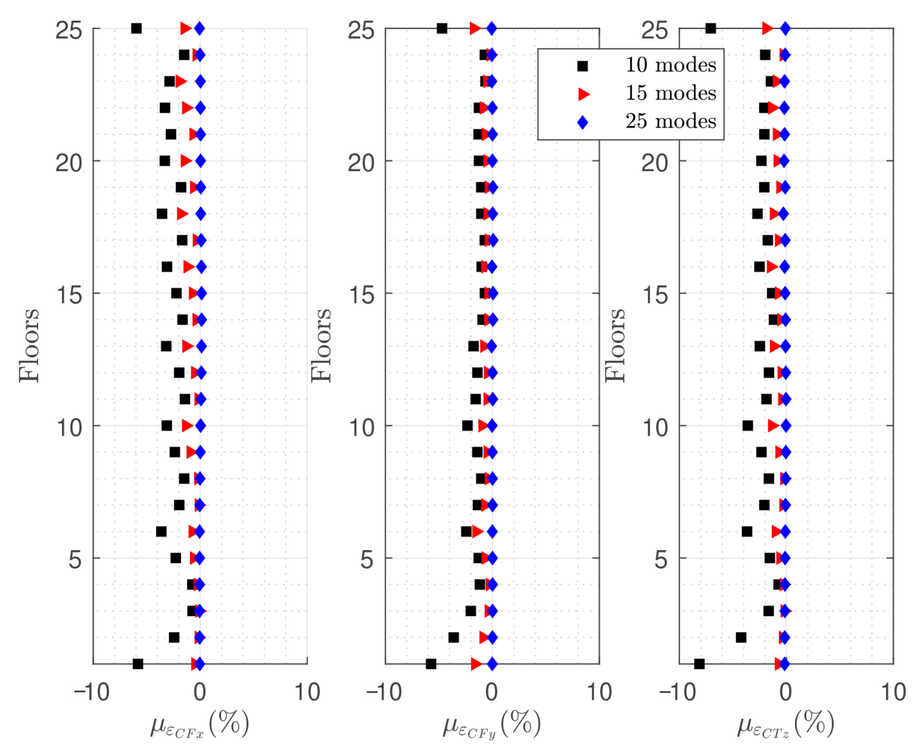
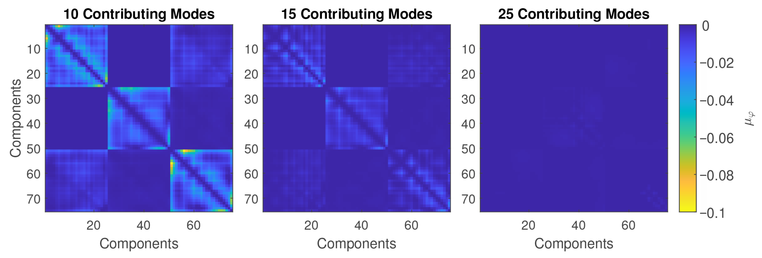
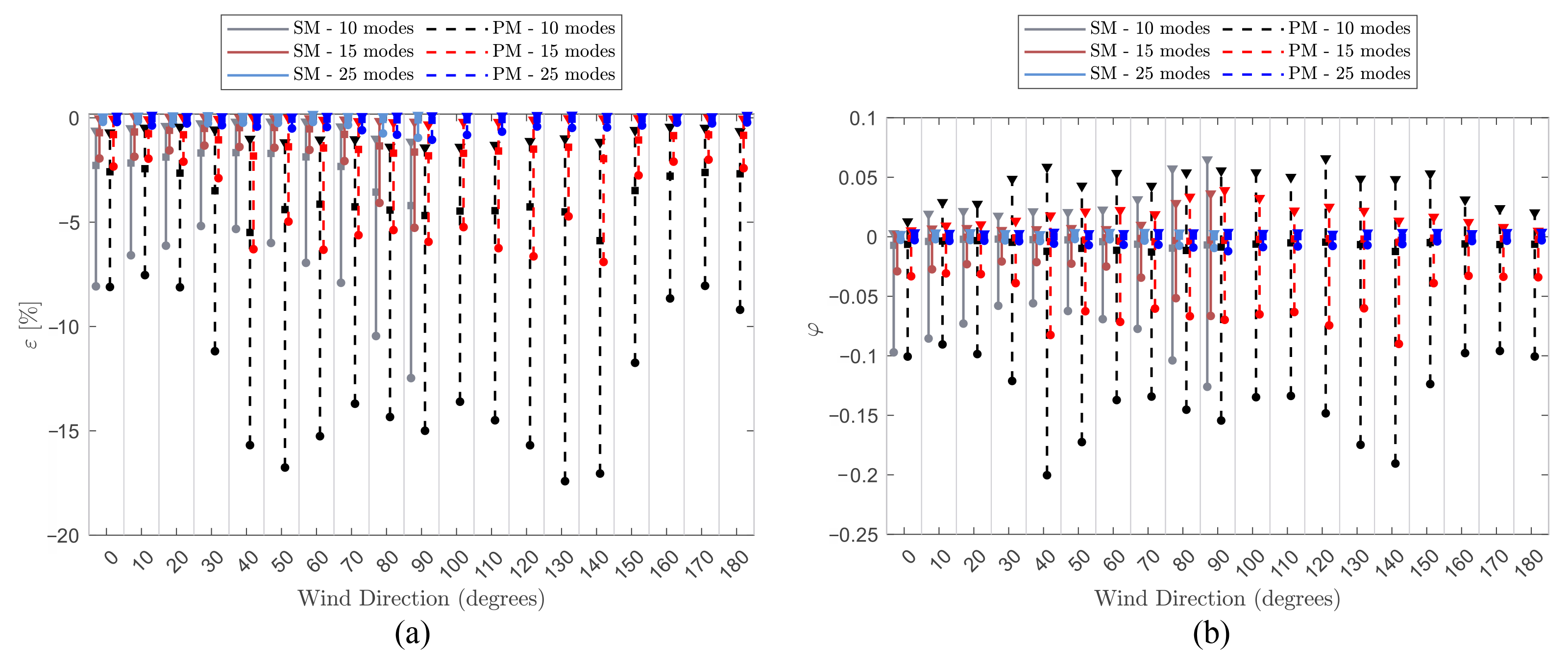
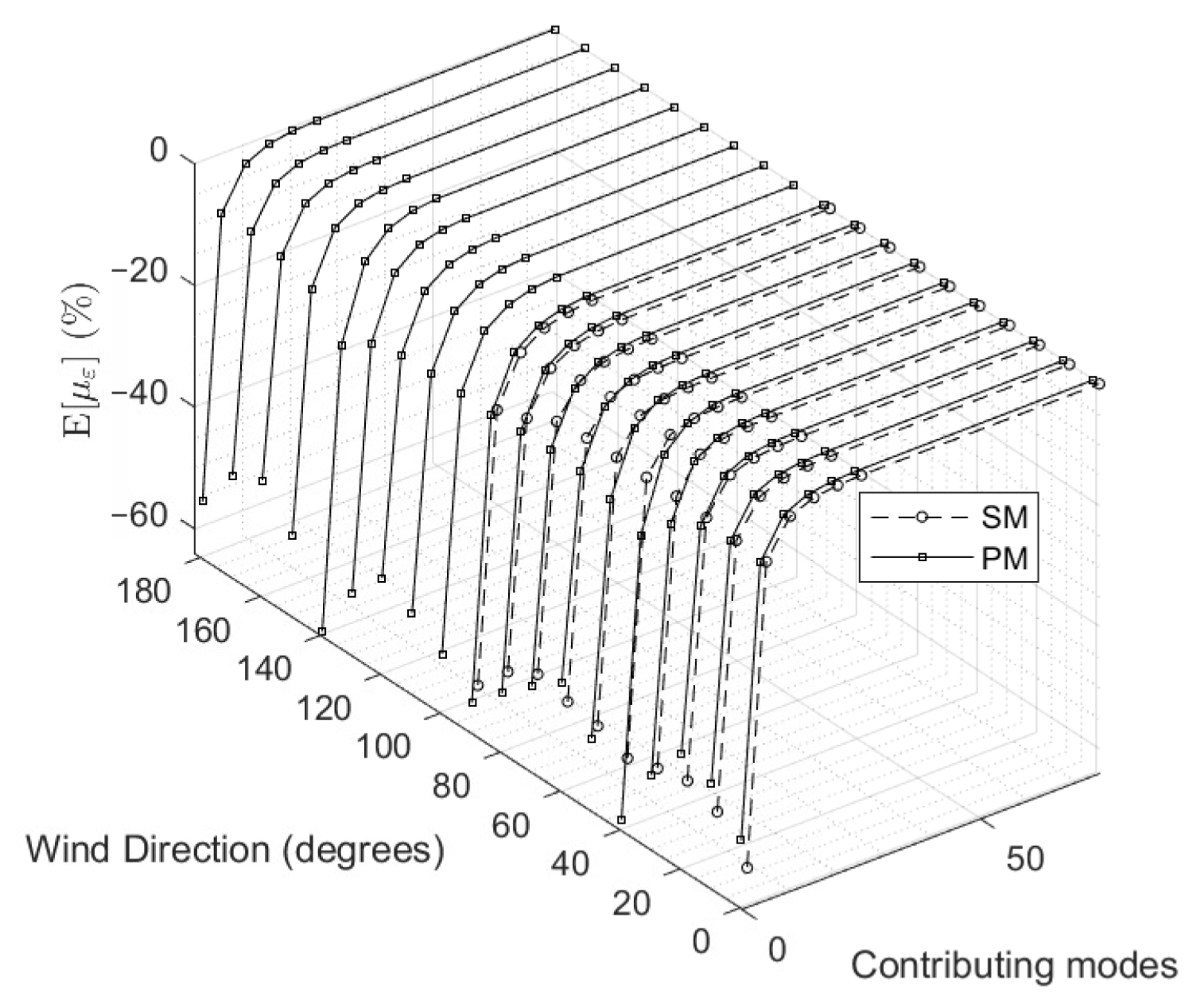
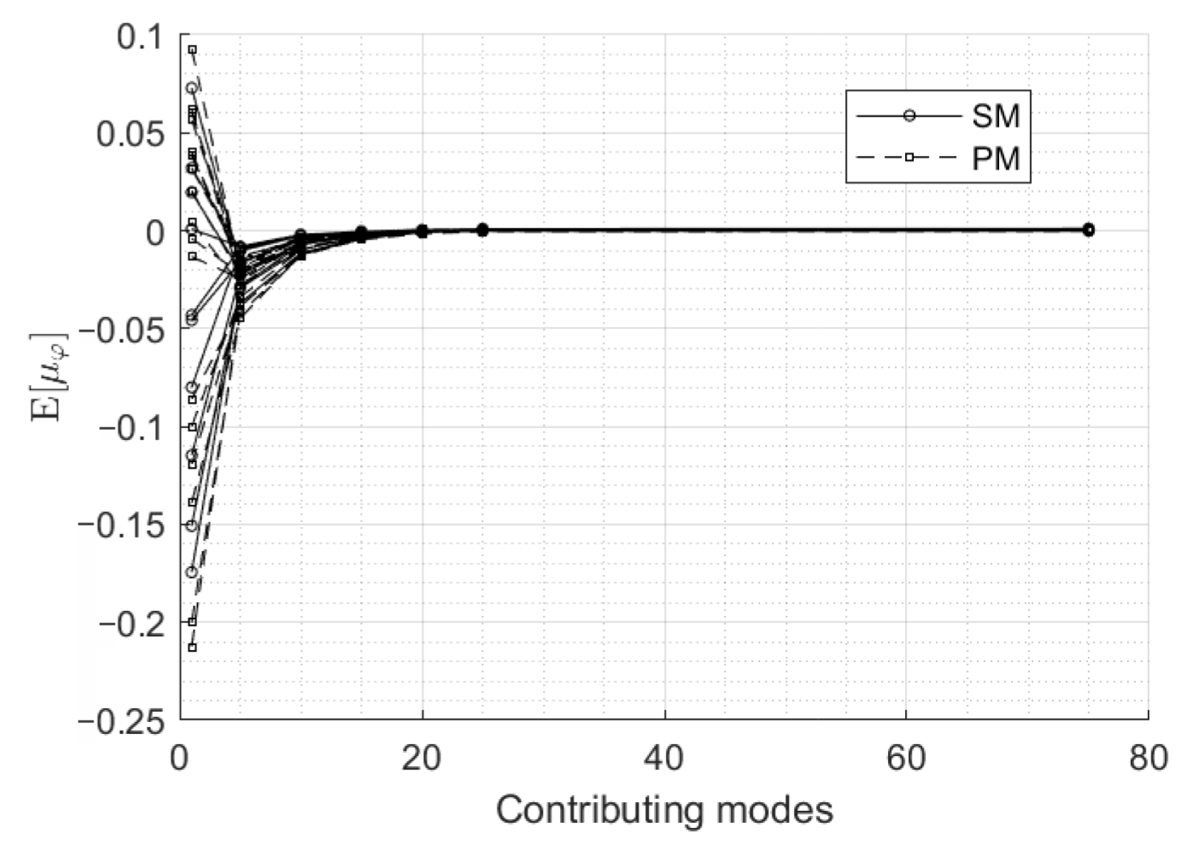
5.3.2. Truncation Errors

To study the effects of mode truncation, the simulation of a set of 40,000 realizations was conducted, using the wind-tunnel-informed stochastic wind load model calibrated to the target spectra. This was used to carry out a parametric study varying the number of modes, in order to examine the errors this induced in the variance and the correlation coefficients.
A total of 10, 15, and 25 out of the 75 total modes were considered, to generate samples for the SM layout and wind direction β = 0 , which corresponded to 13%, 20%, and 33% of all modes, respectively. The value of μ ε , shown in Figure 18, reduced as the number of modes increased, as expected. Figure 19 shows how the map of μ φ changes for an increase in the number of contributing modes. The results demonstrate that consideration of the lower modes associated with large eigenvalues is crucial for capturing the majority of the energy of the process, while consideration of higher modes does not significantly improve accuracy. This result agrees with other studies in the literature for multiple applications [12,15,26].
Figure 20a,b summarize the statistics (i.e., maximum, minimum, and expected values) of ε and φ , for the various wind directions and two configurations. For a reduced number of modes, i.e., 10 and 15 modes, the errors were considerably larger and more sensitive to changes in wind directions and configurations. However, for a sufficient number of contributing modes, i.e., 25 modes, the errors were sufficiently small for all cases. This confirms that a minimum number of modes in the simulation is necessary to ensure small and consistent errors, given any wind direction and configuration.
Figure 21 and Figure 22 show the expected values of μ ε and the expected values of μ φ for all wind directions and both experimental settings, considering varying numbers of contributing modes. The results demonstrate that the wind-tunnel-informed stochastic model is able to accurately simulate reduced-order signals, regardless of the type of input spectra. For the test conditions investigated in this study, it is possible to observe that E [ μ ε ] reached a value between −0.2% to −0.6% for approximately 20 modes (i.e., around 27% of all modes) while E [ μ φ ] reached a value of around 10 4 , which is comparable to the model error, considering all modes. This means that higher modes do not have a significant contribution to the loading process and can be truncated with no noticeable loss of accuracy. Similar results have been encountered in different studies, where for local loads and pressures about 20% to 30% of modes were necessary to provide high accuracy [12,15].

6. Conclusions and Discussion

An extensive wind tunnel test campaign was conducted, considering multiple wind directions and two different experimental configurations, to ultimately quantify the uncertainties introduced in the simulation of wind loads when using typical single short-duration wind tunnel records to calibrate POD-based stochastic wind load models. A discussion on the limitations of using data-informed POD models has also been provided, with respect to model errors and the truncation of higher-order modes.
The major contributions of this study are as follows. We have demonstrated that the spectra estimated from single short-duration wind load records can considerably deviate from the spectra of the underlying stochastic process, even when smoothing is applied to reduce noise. The standard deviation of the errors in the variance estimated from the integration of the spectra can reach 12%, while the standard deviation of the errors in the correlation coefficients can reach values as high as 0.08. This significant variability supports the argument that uncertainty should be considered when simulating wind loads calibrated to spectral functions estimated from single short-duration records, because it can affect the response estimates of wind-excited systems. Moreover, we observed that errors introduced by the use of single short-duration records are of a similar magnitude for different experimental conditions, with no particular sensitivity to the experimental setting being observed. We also found that errors in the variance have a high correlation for forces acting in the same direction, whereas for forces acting in different directions these errors have a low-to-moderate correlation. Lastly, we have demonstrated that the wind-tunnel-informed stochastic wind load model has negligible model errors, as compared to the errors introduced by calibration to single short-duration records. Regarding mode truncation, we observed that at least 25% of modes should be included for simulating wind loads for the tested scenarios with negligible errors, which, overall, is consistent with the results found in the literature. It is important to note that even though 19 cases were considered, the study of the effects of the uncertainties of this work should be investigated for other geometries and record durations, in order to obtain a more comprehensive uncertainty quantification.
To conclude, due to its straightforwardness, the wind-tunnel-informed stochastic wind load model can be a powerful alternative to reduce the reliance on the collection of multiple wind records for generating representative samples of stochastic wind load time series. It is hoped that the extensive error analysis associated with the use of the data-driven POD-based stochastic wind load model of this work will provide greater confidence for the use of such models in wind engineering applications—in particular, for structural response estimation, performance-based wind engineering, and vibration control. Future research efforts will focus on expanding the error assessment of this work to non-Gaussian multivariate wind processes, developing models that incorporate these uncertainties in probabilistic performance assessment approaches, and quantifying the impacts of these uncertainties on the structural response.

Author Contributions

Conceptualization, A.S. and S.M.J.S.; methodology, A.S. and S.M.J.S.; validation, T.G.A.D. and S.A.; formal analysis, T.G.A.D.; resources, A.S. and S.M.J.S.; data curation, T.G.A.D. and S.A.; writing—original draft preparation, T.G.A.D.; writing—review and editing, S.A., A.S. and S.M.J.S.; visualization, T.G.A.D.; supervision, A.S. and S.M.J.S.; project administration, A.S. and S.M.J.S.; funding acquisition, A.S. and S.M.J.S. All authors have read and agreed to the published version of the manuscript.

Funding

This research was funded by the National Science Foundation, Grants: CMMI-1750339, CMMI-2118488, and CMMI-2131111.

Institutional Review Board Statement

Not applicable.

Informed Consent Statement

Not applicable.

Data Availability Statement

The wind tunnel data generated for this study are published in the Design Safe Database and can be accessed free of charge.

Acknowledgments

The authors would like to acknowledge Sungmoon Jung for providing the scale model used in this study.

Conflicts of Interest

The authors declare no conflict of interest.

Appendix A. Standardization Scheme of Force Coefficients

To increase the efficiency of carrying out a POD analysis of wind force coefficients, it is first advisable to standardize the data. To this end, the zero-mean force coefficients were standardized in this study, using the following scheme:
C F x , n n o r m ( t ) = C F x , n ( t ) σ C F x , n γ r
C F y , n n o r m ( t ) = C F y , n ( t ) σ C F y , n γ r
C T z , n n o r m ( t ) = C T z , n ( t ) σ C T z , n γ r
where C F x ( t ) , C F y ( t ) , and C T z ( t ) , are the zero-mean force coefficients, while γ r = 3.5 is the reduced variate estimated based on the expected peak of a Gaussian process after normalization. As an example, Figure A1 illustrates the standardized force coefficient time series of an individual record for wind direction β = 0 and the SM layout.
Figure A1. Example time series of the standardized force coefficients for β = 0 and the SM layout.
Wind 03 00022 g0a1

References

  1. Zeldin, B.A.; Spanos, P.D. Random Field Representation and Synthesis Using Wavelet Bases. J. Appl. Mech. 1996, 63, 946–952. [Google Scholar] [CrossRef]
  2. Kitagawa, T.; Nomura, T. A wavelet-based method to generate artificial wind fluctuation data. J. Wind Eng. Ind. Aerodyn. 2003, 91, 943–964. [Google Scholar] [CrossRef]
  3. Li, Y.; Kareem, A. Simulation of multivariate random processes: Hybrid DFT and digital filtering approach. J. Eng. Mech. 1993, 119, 1078–1098. [Google Scholar] [CrossRef]
  4. Mignolet, M.P.; Spanos, P.D. Simulation of Homogeneous Two-Dimensional Random Fields: Part I—AR and ARMA Models. J. Appl. Mech. 1992, 59, S260–S269. [Google Scholar] [CrossRef]
  5. Shinozuka, M.; Deodatis, G. Simulation of stochastic processes by spectral representation. Appl. Mech. Rev. 1991, 44, 191–204. [Google Scholar] [CrossRef]
  6. Deodatis, G. Simulation of ergodic multivariate stochastic processes. J. Eng. Mech. 1996, 122, 778–787. [Google Scholar] [CrossRef]
  7. Cheynet, E.; Daniotti, N.; Bogunović Jakobsen, J.; Snæbjörnsson, J.; Wang, J. Unfrozen skewed turbulence for wind loading on structures. Appl. Sci. 2022, 12, 9537. [Google Scholar] [CrossRef]
  8. Huang, G.; Peng, L.; Kareem, A.; Song, C. Data-driven simulation of multivariate nonstationary winds: A hybrid multivariate empirical mode decomposition and spectral representation method. J. Wind Eng. Ind. Aerodyn. 2020, 197, 104073. [Google Scholar] [CrossRef]
  9. López-Ibarra, A.; Pozos-Estrada, A.; Nava-González, R. Effect of Partially Correlated Wind Loading on the Response of Two-Way Asymmetric Systems: The Impact of Torsional Sensitivity and Nonlinear Effects. Appl. Sci. 2023, 13, 6421. [Google Scholar] [CrossRef]
  10. Wang, L.; McCullough, M.; Kareem, A. A data-driven approach for simulation of full-scale downburst wind speeds. J. Wind Eng. Ind. Aerodyn. 2013, 123, 171–190. [Google Scholar] [CrossRef]
  11. Shinozuka, M. Stochastic fields and their digital simulation. In Stochastic Methods in Structural Dynamics; Springer: Dordrecht, The Netherlands, 1987; pp. 93–133. [Google Scholar]
  12. Tamura, Y.; Suganuma, S.; Kikuchi, H.; Hibi, K. Proper orthogonal decomposition of random wind pressure field. J. Fluids Struct. 1999, 13, 1069–1095. [Google Scholar] [CrossRef]
  13. Carassale, L.; Piccardo, G.; Solari, G. Double modal transformation and wind engineering applications. J. Eng. Mech. 2001, 127, 432–439. [Google Scholar] [CrossRef]
  14. Chen, L.; Letchford, C.W. Simulation of multivariate stationary Gaussian stochastic processes: Hybrid spectral representation and proper orthogonal decomposition approach. J. Eng. Mech. 2005, 131, 801–808. [Google Scholar] [CrossRef]
  15. Chen, X.; Kareem, A. Proper orthogonal decomposition-based modeling, analysis, and simulation of dynamic wind load effects on structures. J. Eng. Mech. 2005, 131, 325–339. [Google Scholar] [CrossRef]
  16. Ouyang, Z.; Spence, S.M.J. A performance-based wind engineering framework for envelope systems of engineered buildings subject to directional wind and rain hazards. J. Struct. Eng. 2020, 146, 04020049. [Google Scholar] [CrossRef]
  17. Hu, L.; Li, L.; Gu, M. Error assessment for spectral representation method in wind velocity field simulation. J. Eng. Mech. 2010, 136, 1090–1104. [Google Scholar] [CrossRef]
  18. Tao, T.; Wang, H.; Hu, L.; Kareem, A. Error analysis of multivariate wind field simulated by interpolation-enhanced spectral representation method. J. Eng. Mech. 2020, 146, 04020049. [Google Scholar] [CrossRef]
  19. Davenport, A. The response of six building shapes to turbulent wind. Philos. Trans. R. Soc. Lond. A Math. Phys. Eng. Sci. 1971, 269, 385–394. [Google Scholar]
  20. Simiu, E. Wind spectra and dynamic alongwind response. J. Struct. Div. 1974, 100, 1897–1910. [Google Scholar] [CrossRef]
  21. Melbourne, W. Comparison of measurements on the CAARC standard tall building model in simulated model wind flows. J. Wind Eng. Ind. Aerodyn. 1980, 6, 73–88. [Google Scholar] [CrossRef]
  22. Solari, G. Analytical estimation of the alongwind response of structures. J. Wind Eng. Ind. Aerodyn. 1983, 14, 467–477. [Google Scholar] [CrossRef]
  23. Kaimal, J.C.; Finnigan, J.J. Atmospheric Boundary Layer Flows: Their Structure and Measurement; Oxford University Press: Oxford, UK, 1994. [Google Scholar]
  24. Gurley, K.; Kareem, A. Simulation of correlated non-Gaussian pressure fields. Meccanica 1998, 33, 309–317. [Google Scholar] [CrossRef]
  25. Suksuwan, A.; Spence, S.M.J. Optimization of uncertain structures subject to stochastic wind loads under system-level first excursion constraints: A data-driven approach. Comput. Struct. 2018, 210, 58–68. [Google Scholar] [CrossRef]
  26. Lin, N.; Letchford, C.; Tamura, Y.; Liang, B.; Nakamura, O. Characteristics of wind forces acting on tall buildings. J. Wind Eng. Ind. Aerodyn. 2005, 93, 217–242. [Google Scholar] [CrossRef]
  27. Tamura, Y.; Kareem, A. Advanced Structural Wind Engineering; Springer: Tokyo, Japan, 2013; Volume 482. [Google Scholar]
  28. Spence, S.M.J.; Kareem, A. Data-enabled design and optimization (DEDOpt): Tall steel building frameworks. Comput. Struct. 2013, 129, 134–147. [Google Scholar] [CrossRef]
  29. Gurley, K.R. Modelling and Simulation of Non-Gaussian Processes; University of Notre Dame: Notre Dame, IN, USA, 1997. [Google Scholar]
  30. Welch, P. The use of fast Fourier transform for the estimation of power spectra: A method based on time averaging over short, modified periodograms. IEEE Trans. Audio Electroacoust. 1967, 15, 70–73. [Google Scholar] [CrossRef]
  31. Solomon, O.M., Jr. PSD Computations Using Welch’s Method; Technical Report; Sandia National Labs.: Albuquerque, NM, USA, 1991. [Google Scholar]
  32. Tao, T.; Wang, H.; Yao, C.; He, X.; Kareem, A. Efficacy of interpolation-enhanced schemes in random wind field simulation over long-span bridges. J. Bridge Eng. 2018, 23, 04017147. [Google Scholar] [CrossRef]
  33. Catarelli, R.A.; Fernández-Cabán, P.L.; Phillips, B.M.; Bridge, J.A.; Masters, F.J.; Gurley, K.R.; Prevatt, D.O. Automation and new capabilities in the university of Florida NHERI Boundary Layer Wind Tunnel. Front. Built Environ. 2020, 6, 558151. [Google Scholar] [CrossRef]
  34. Wu, Y.; Gao, Y.; Li, D. Error assessment of multivariate random processes simulated by a conditional-simulation method. J. Eng. Mech. 2015, 141, 04014155. [Google Scholar] [CrossRef]
Figure 1. (a) illustration of the building model used in the wind tunnel tests, and configuration of the pressure taps, (b) wind tunnel testing with SM setup, and (c) wind tunnel testing with PM setup.
Wind 03 00022 g001
Figure 2. (a) SM setup, (b) PM setup, and (c) coordinate system adopted in estimating the wind loads.
Wind 03 00022 g002
Figure 3. Representation of the UF NHERI boundary layer wind tunnel.
Wind 03 00022 g003
Figure 4. Comparison between smoothed PSDs of short-duration records, S R ( f ) , and target PSD of C F x , 20 ( t ) at the 20th floor and wind direction of β = 0 .
Wind 03 00022 g004
Figure 5. Comparison between smoothed PSDs of short-duration records, S R ( f ) , and target PSD of C F y , 20 ( t ) at the 20th floor and wind direction of β = 0 .
Wind 03 00022 g005
Figure 6. Comparison between smoothed PSDs of short-duration records, S R ( f ) , and target PSD of C T z , 20 ( t ) at the 20th floor and wind direction of β = 0 .
Wind 03 00022 g006
Figure 7. Mean error in the variance, μ ε , with standard deviation, σ ε , for each floor, for the SM layout and β = 0 .
Wind 03 00022 g007
Figure 8. (a) mean errors in the variance for SM and PM layouts, and (b) standard deviation of the errors in the variance for the SM and PM layouts.
Wind 03 00022 g008
Figure 9. Map of the target correlation coefficients for the SM setup and wind direction β = 0 .
Wind 03 00022 g009
Figure 10. Mean error in the correlation coefficients for the SM setup and wind direction β = 0 .
Wind 03 00022 g010
Figure 11. Standard deviation of the difference between target and typical correlation coefficients for the SM setup and wind direction β = 0 .
Wind 03 00022 g011
Figure 12. (a) mean errors in the correlation coefficients for SM and PM layouts, and (b) standard deviation of the errors in the correlation coefficients for the SM and PM layouts.
Wind 03 00022 g012
Figure 13. Histograms of ε associated with SM layout and β = 0 of (a) C F x , (b) C F y , (c) C T z , and (d) correlation coefficients between the components of ε .
Wind 03 00022 g013
Figure 14. Expected values and range of the model error in the variance for the SM and PM setups.
Wind 03 00022 g014
Figure 15. Expected values and range of the model error in the correlation coefficients for the SM and PM setups.
Wind 03 00022 g015
Figure 16. Comparison of the error in the variance due to the use of a single smoothed short-duration wind tunnel record (wt) and the simulation model (sim).
Wind 03 00022 g016
Figure 17. Comparison of the difference between the correlation coefficients due to the use of a single smoothed short-duration wind tunnel record (wt) and the simulation model (sim).
Wind 03 00022 g017
Figure 18. Mean error in the variance, μ ε , for each force coefficient component, considering 10, 15, and 25 contributing modes, for SM layout and wind direction β = 0 .
Wind 03 00022 g018
Figure 19. Mean error in the correlation coefficients, considering 10, 15, and 25 modes, for SM layout and wind direction β = 0 .
Wind 03 00022 g019
Figure 20. (a) error in the variance, ε , and (b) errors in the correlation coefficients, φ , considering 10, 15, and 25 contributing modes.
Wind 03 00022 g020
Figure 21. Expected error in the variance from the truncation of modes for both the SM and PM setups, considering 1, 5, 10, 15, 20, 25, and 75 contributing modes.
Wind 03 00022 g021
Figure 22. Expected difference in the correlation coefficients from the truncation of modes for all wind directions and the SM and PM setups, considering 1, 5, 10, 15, 20, 25, and 75 contributing modes.
Wind 03 00022 g022
Disclaimer/Publisher’s Note: The statements, opinions and data contained in all publications are solely those of the individual author(s) and contributor(s) and not of MDPI and/or the editor(s). MDPI and/or the editor(s) disclaim responsibility for any injury to people or property resulting from any ideas, methods, instructions or products referred to in the content.

