
Investigation and Optimisation of High-Lift Airfoils for Airborne Wind Energy Systems at High Reynolds Numbers

Abstract
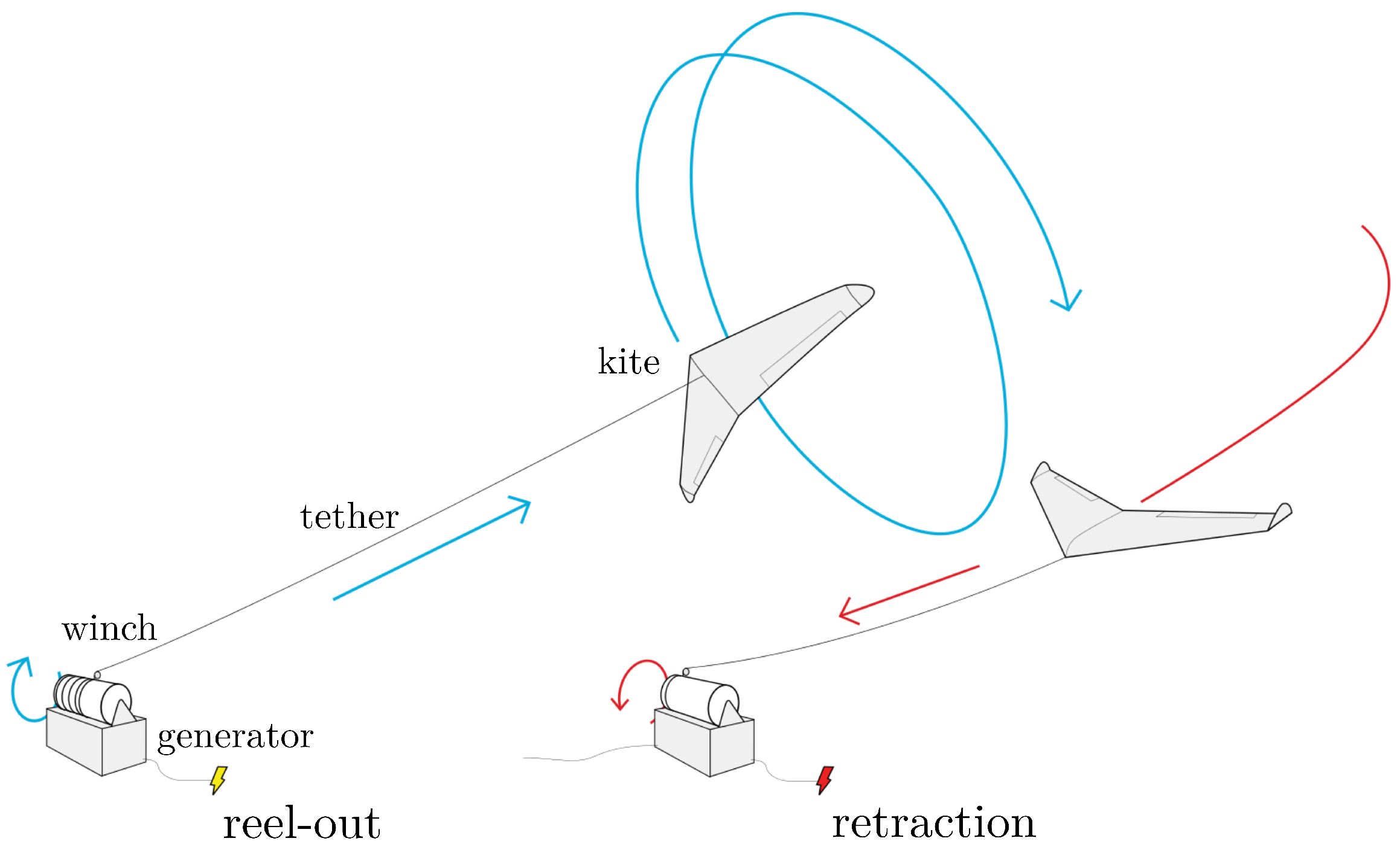
:1. Introduction
2. Design Process
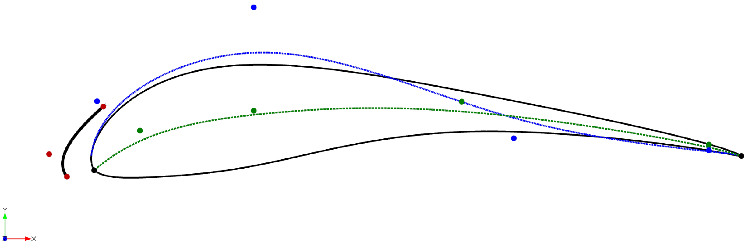
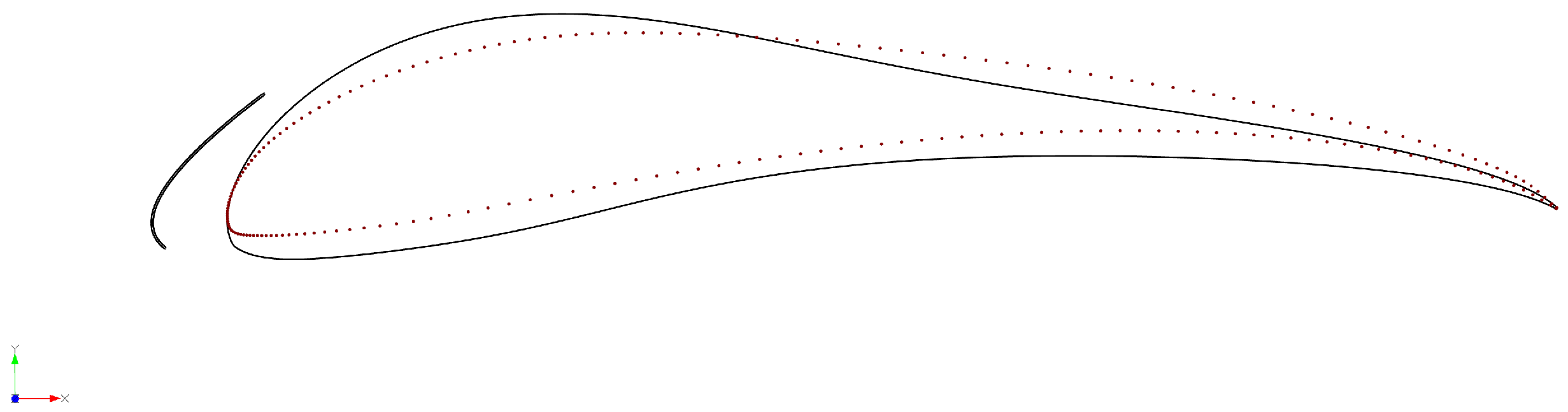
2.1. Parametrisation
2.2. Optimisation Process
- Algorithm
- Objectives
- Design Parameters
- Constraints
2.3. Numerical Setup for Optimisation Evaluations
2.4. Preliminary Geometry
3. Numerical Setup
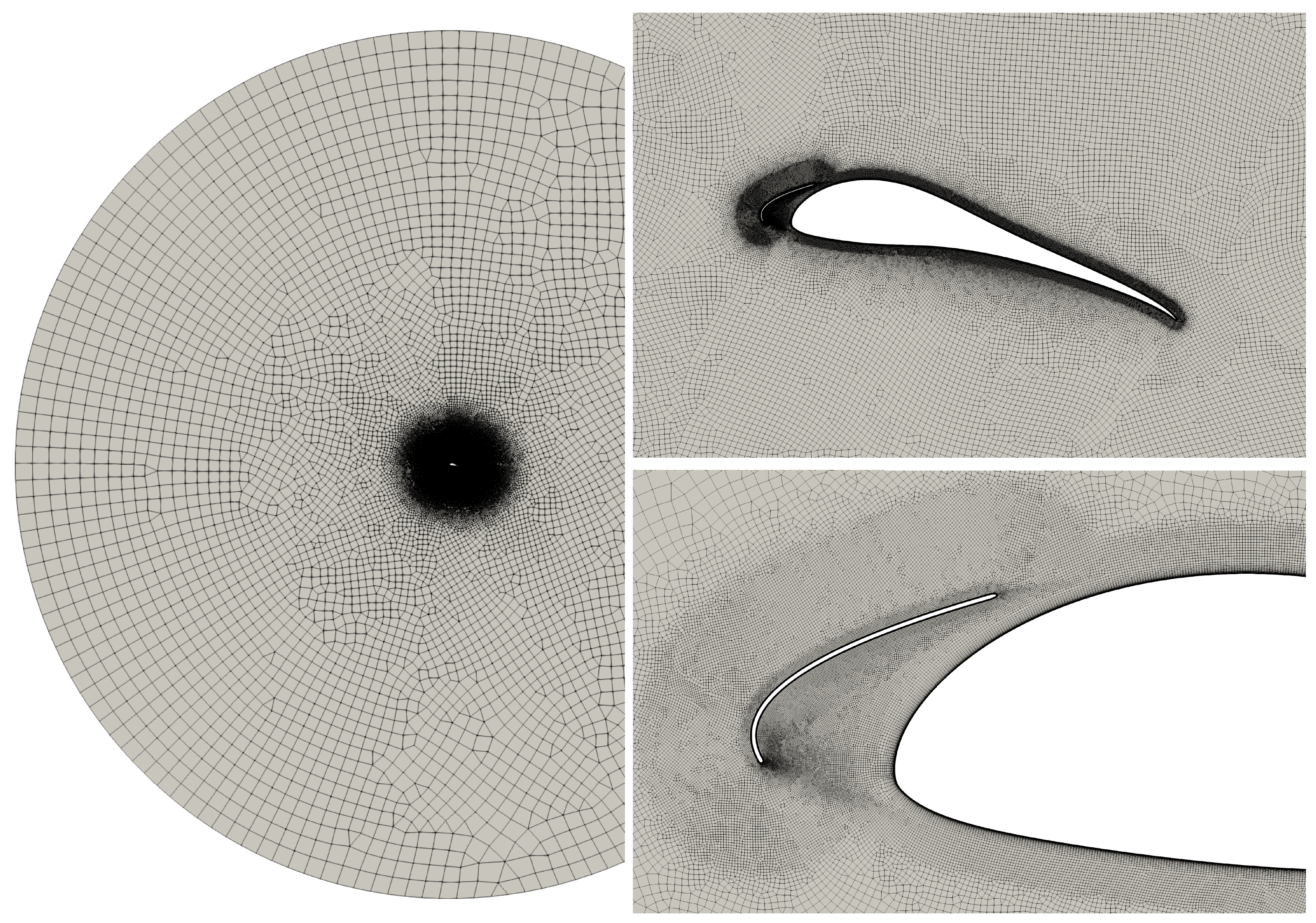
3.1. Mesh
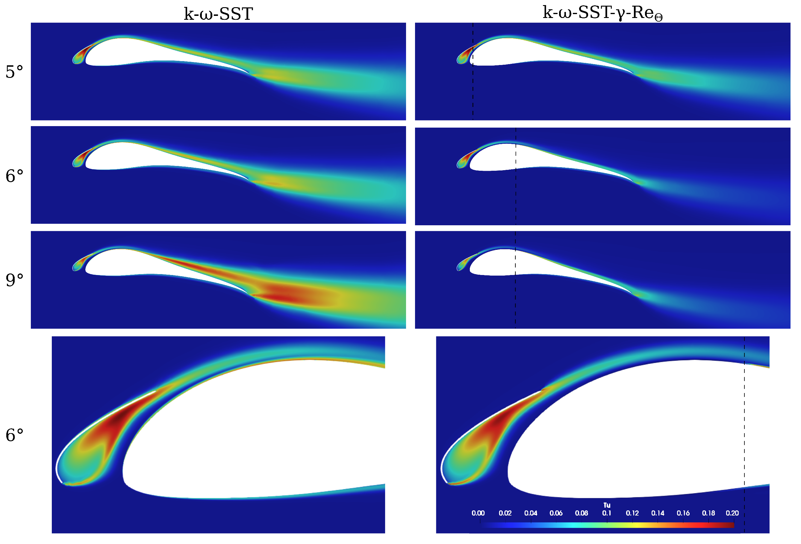
3.2. Turbulence Model
4. Experiment Setup
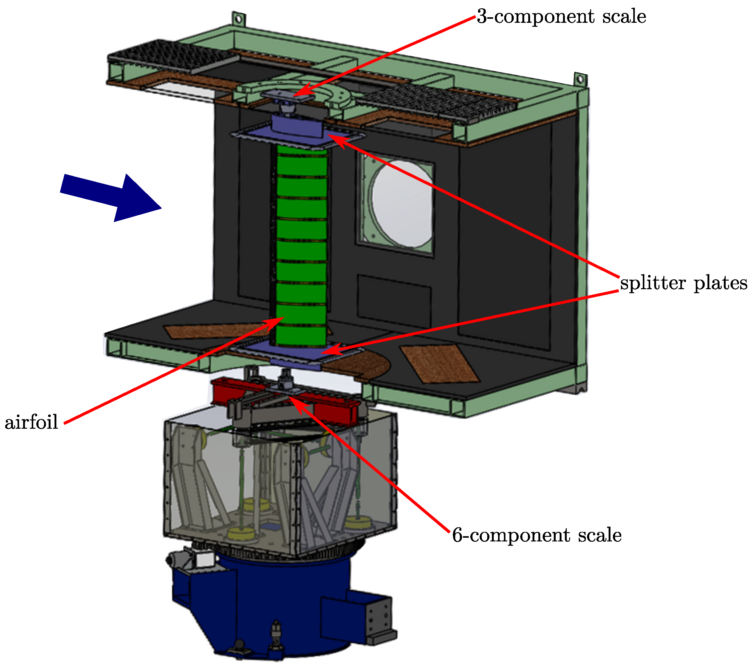
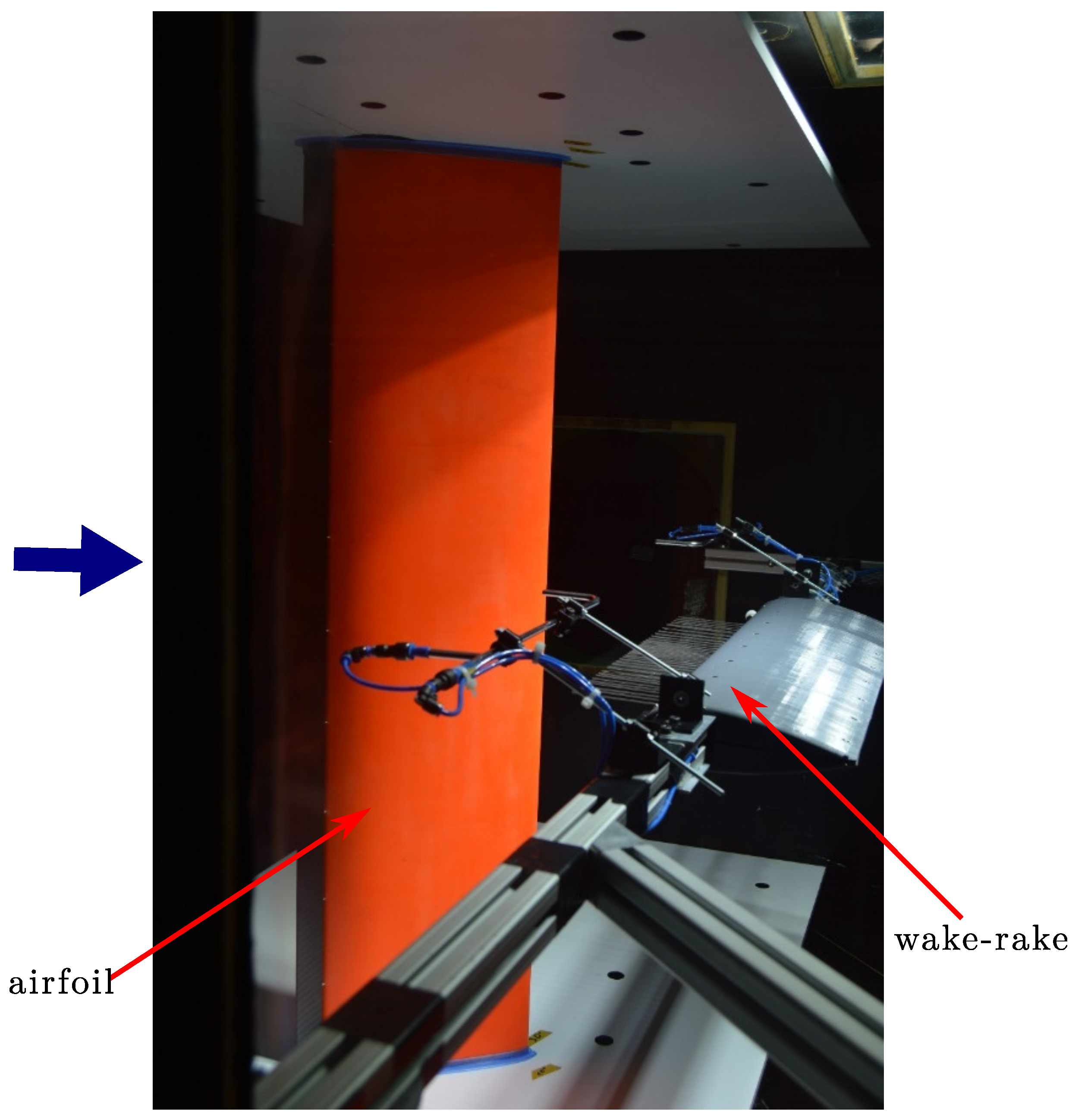
4.1. Facilities and Measurement Techniques
- Force Measurements
- Pressure Measurements
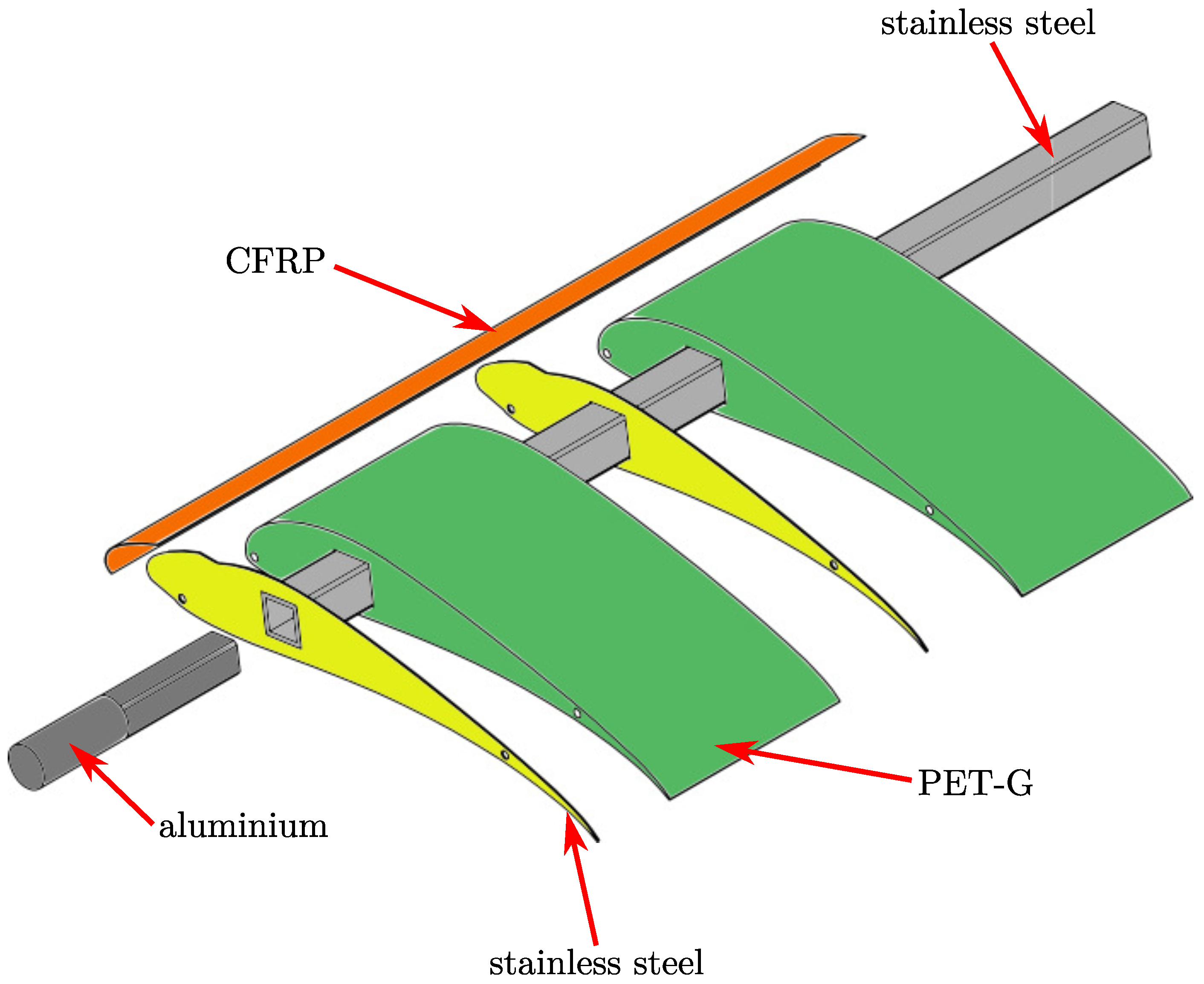
4.2. Model Airfoils
5. Results
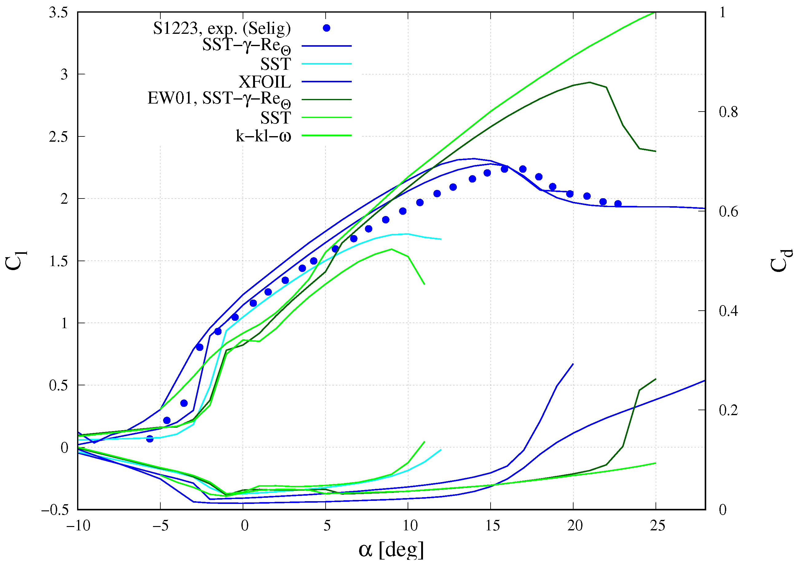
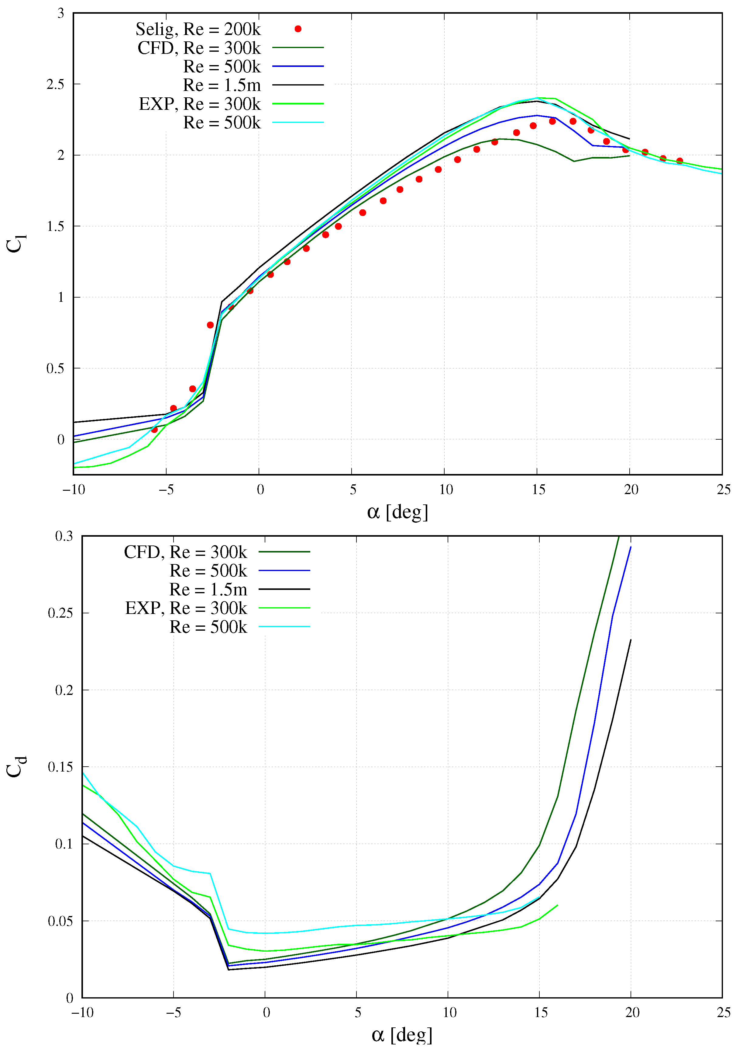
5.1. Baseline Airfoil (S1223)
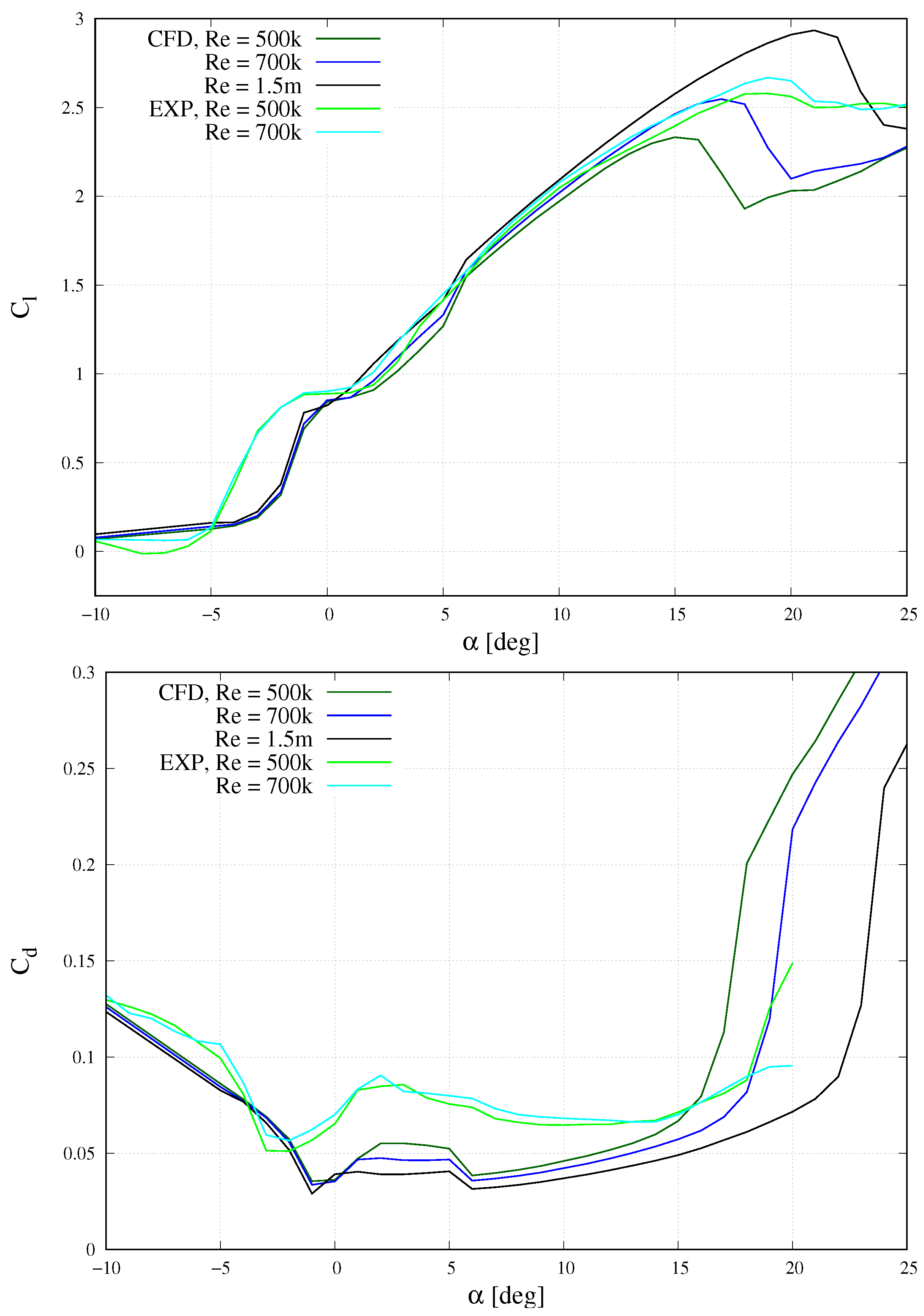
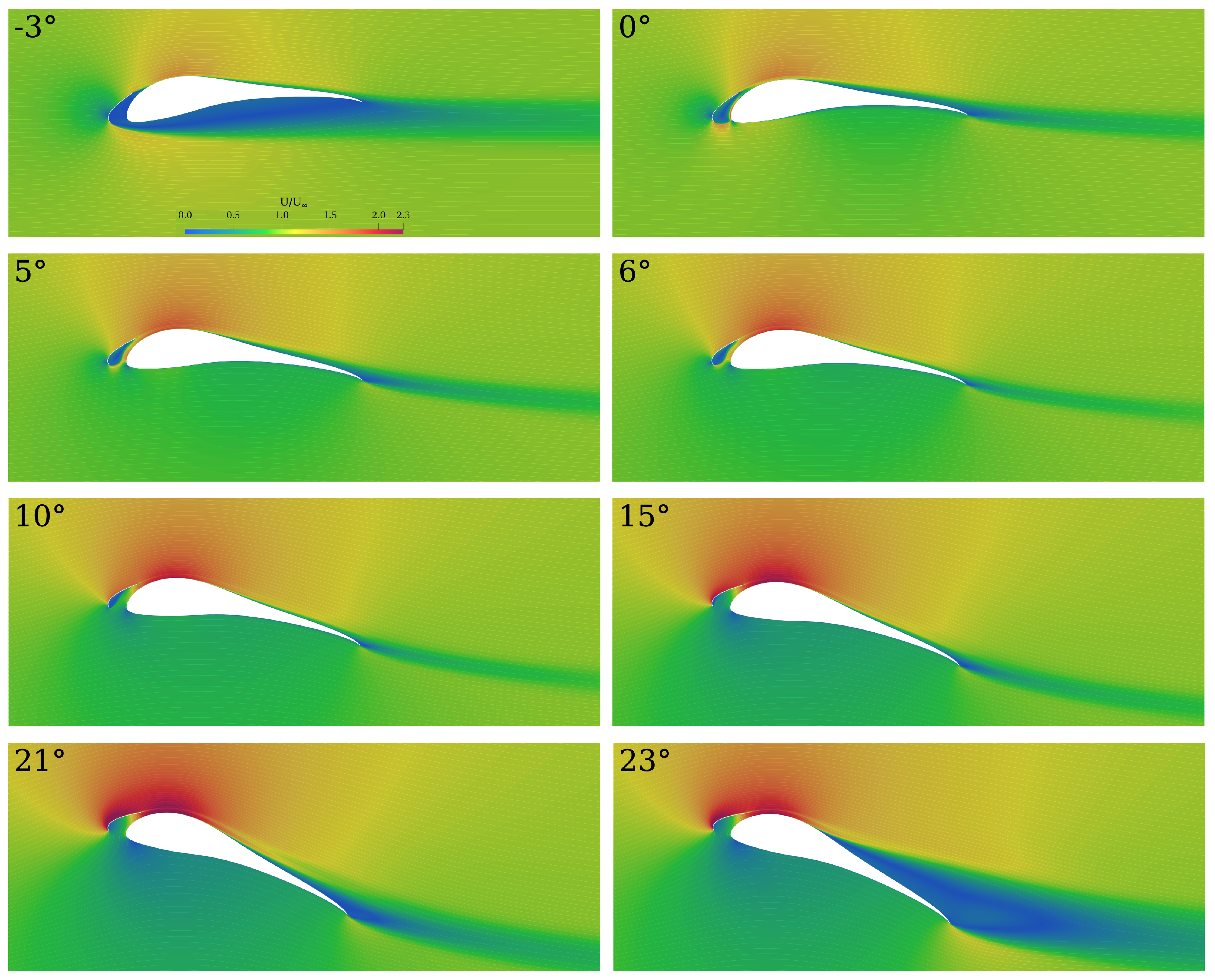
5.2. Optimised Airfoil with Slat (EW01)
6. Discussion
7. Summary and Conclusions
Author Contributions
Funding
Data Availability Statement
Acknowledgments
Conflicts of Interest
Abbreviations
| AWE | Airborne wind energy |
| CFD | Computational fluid dynamics |
| RANS | Reynolds-averaged Navier-Stokes |
| SST | Shear stress transport |
| EW01 | name for optimised airfoil and slat |
| IDDES | Improved delayed detached eddy simulation |
| GroWiKa | Large wind tunnel at TU Berlin |
| GFRP | Glass-fiber reinforced plastic |
| CFRP | Carbon-fiber reinforced plastic |
| FDM | Fused deposition modeling |
| PET-G | Polyethylene terephthalate |
References
- European Commission, Directorate General for Research and Innovation. Study on Challenges in the Commercialisation of Airborne Wind Energy Systems; Publications Office: Luxemburg, 2018. [Google Scholar] [CrossRef]
- Zillmann, U.; Bechtle, P. Emergence and Economic Dimension of Airborne Wind Energy. In Airborne Wind Energy: Advances in Technology Development and Research; Schmehl, R., Ed.; Springer: Singapore, 2018; pp. 1–25. [Google Scholar] [CrossRef]
- Vermillion, C.; Cobb, M.; Fagiano, L.; Leuthold, R.; Diehl, M.; Smith, R.S.; Wood, T.A.; Rapp, S.; Schmehl, R.; Olinger, D.; et al. Electricity in the air: Insights from two decades of advanced control research and experimental flight testing of airborne wind energy systems. Annu. Rev. Control 2021, 52, 330–357. [Google Scholar] [CrossRef]
- Schmidt, H.; de Vries, G.; Renes, R.J.; Schmehl, R. The Social Acceptance of Airborne Wind Energy: A Literature Review. Energies 2022, 15, 1384. [Google Scholar] [CrossRef]
- Cherubini, A.; Papini, A.; Vertechy, R.; Fontana, M. Airborne Wind Energy Systems: A review of the technologies. Renew. Sustain. Energy Rev. 2015, 51, 1461–1476. [Google Scholar] [CrossRef] [Green Version]
- Ahrens, U. Airborne Wind Energy: An Overview of the Technological Approaches; Springer International Publishing: Berlin/Heidelberg, Germany, 2023. [Google Scholar] [CrossRef]
- Licitra, G.; Koenemann, J.; Bürger, A.; Williams, P.; Ruiterkamp, R.; Diehl, M. Performance assessment of a rigid wing Airborne Wind Energy pumping system. Energy 2019, 173, 569–585. [Google Scholar] [CrossRef]
- Pereira, A.F.C.; Sousa, J.M.M. A Review on Crosswind Airborne Wind Energy Systems: Key Factors for a Design Choice. Energies 2022, 16, 351. [Google Scholar] [CrossRef]
- Fagiano, L.; Quack, M.; Bauer, F.; Carnel, L.; Oland, E. Autonomous Airborne Wind Energy Systems: Accomplishments and Challenges. Annu. Rev. Control. Robot. Auton. Syst. 2022, 5, 603–631. [Google Scholar] [CrossRef]
- Airborne Wind Europe. About Airborne Wind Energy. Available online: http://web.archive.org/web/20230307170451/https://airbornewindeurope.org/about-airborne-wind-energy/ (accessed on 22 February 2023).
- Loyd, M.L. Crosswind kite power (for large-scale wind power production). J. Energy 1980, 4, 106–111. [Google Scholar] [CrossRef]
- Selig, M.S.; Guglielmo, J.J. High-Lift Low Reynolds Number Airfoil Design. J. Aircr. 1997, 34, 72–79. [Google Scholar] [CrossRef] [Green Version]
- Althaus, D.; Wortmann, F.X. Stuttgarter Profilkatalog: Messergebnisse aus dem Laminarwindkanal des Instituts für Aerodynamik und Gasdynamik der Universität Stuttgart; Vieweg: Kranzberg, Germany, 1981; Volume 1. [Google Scholar]
- Imumbhon, J.O.; Alam, M.D.; Cao, Y. Design and Structural Analyses of a Reciprocating S1223 High-Lift Wing for an RA-Driven VTOL UAV. Aerospace 2021, 8, 214. [Google Scholar] [CrossRef]
- Drela, M. XFOIL: An analysis and design system for low Reynolds number airfoils. In Low Reynolds Number Aerodynamics, Proceedings of the Conference Notre Dame, Indiana, USA, 5–7 June 1989; Springer: Berlin/Heidelberg, Germany, 1989. [Google Scholar]
- Selig, M.S. (Ed.) Summary of Low Speed Airfoil Data; SoarTech Publications: Virginia Beach, VA, USA, 1995. [Google Scholar]
- Viré, A.; LeBlanc, B.; Steiner, J.; Timmer, N. Experimental study of the effect of a slat on the aerodynamic performance of a thick base airfoil. Wind. Energy Sci. 2022, 7, 573–584. [Google Scholar] [CrossRef]
- Zaki, A.; Abdelrahman, M.; Ayad, S.S.; Abdellatif, O. Effects of leading edge slat on the aerodynamic performance of low Reynolds number horizontal axis wind turbine. Energy 2022, 239, 122338. [Google Scholar] [CrossRef]
- Chen, T.; Jiang, X.; Wang, H.; Li, Q.; Li, M.; Wu, Z. Investigation of leading-edge slat on aerodynamic performance of wind turbine blade. Proc. Inst. Mech. Eng. Part C J. Mech. Eng. Sci. 2021, 235, 1329–1343. [Google Scholar] [CrossRef]
- Deb, K.; Pratap, A.; Agarwal, S.; Meyarivan, T. A fast and elitist multiobjective genetic algorithm: NSGA-II. IEEE Trans. Evol. Comput. 2002, 6, 182–197. [Google Scholar] [CrossRef] [Green Version]
- Bakar, A.; Li, K.; Liu, H.; Xu, Z.; Alessandrini, M.; Wen, D. Multi-Objective Optimization of Low Reynolds Number Airfoil Using Convolutional Neural Network and Non-Dominated Sorting Genetic Algorithm. Aerospace 2022, 9, 35. [Google Scholar] [CrossRef]
- Drela, M. Newton solution of coupled viscous/inviscid multielement airfoil flows. In Proceedings of the 21st Fluid Dynamics, Plasma Dynamics and Lasers Conference, Seattle, WA, USA, 18–20 June 1990; American Institute of Aeronautics and Astronautics: Seattle, WA, USA, 1990; p. 1470. [Google Scholar] [CrossRef]
- Menter, F.R.; Langtry, R.; Völker, S. Transition Modelling for General Purpose CFD Codes. Flow Turbul. Combust. 2006, 77, 277–303. [Google Scholar] [CrossRef]
- Harries, S.; Abt, C. Integration of Tools for Application Case Studies. In A Holistic Approach to Ship Design: Volume 2: Application Case Studies; Papanikolaou, A., Ed.; Springer International Publishing: Cham, Switzerland, 2021; pp. 7–45. [Google Scholar] [CrossRef]
- Menter, F.R. Two-equation eddy-viscosity turbulence models for engineering applications. AIAA J. 1994, 32, 1598–1605. [Google Scholar] [CrossRef] [Green Version]
- Matyushenko, A.A.; Garbaruk, A.V. Adjustment of the k- ω SST turbulence model for prediction of airfoil characteristics near stall. J. Phys. Conf. Ser. 2016, 769, 012082. [Google Scholar] [CrossRef] [Green Version]
- Khan, S.A.; Bashir, M.; Ali Baig, M.A.; Ghasi Mehaboob Ali, F.A. Comparing the Effect of Different Turbulence Models on The CFD Predictions of NACA0018 Airfoil Aerodynamics. CFD Lett. 2020, 12, 1–10. [Google Scholar] [CrossRef]
- Langtry, R.B.; Menter, F.R. Correlation-Based Transition Modeling for Unstructured Parallelized Computational Fluid Dynamics Codes. AIAA J. 2009, 47, 2894–2906. [Google Scholar] [CrossRef]
- Rogowski, K.; Królak, G.; Bangga, G. Numerical Study on the Aerodynamic Characteristics of the NACA 0018 Airfoil at Low Reynolds Number for Darrieus Wind Turbines Using the Transition SST Model. Processes 2021, 9, 477. [Google Scholar] [CrossRef]
- Barlow, J.B.; Rae, W.H.; Pope, A. Low-Speed Wind Tunnel Testing; John Wiley & Sons: Hoboken, NJ, USA, 1999. [Google Scholar]


| Region | |
|---|---|
| airfoil surface | 0.0015 |
| slat surface | 0.00075 |
| slat leading & trailing edge | 0.0001 |
| refinement area around slat | 0.0015 |
| circular refinement area | 0.01 |
| outer mesh | 1 |
Disclaimer/Publisher’s Note: The statements, opinions and data contained in all publications are solely those of the individual author(s) and contributor(s) and not of MDPI and/or the editor(s). MDPI and/or the editor(s) disclaim responsibility for any injury to people or property resulting from any ideas, methods, instructions or products referred to in the content. |
© 2023 by the authors. Licensee MDPI, Basel, Switzerland. This article is an open access article distributed under the terms and conditions of the Creative Commons Attribution (CC BY) license (https://creativecommons.org/licenses/by/4.0/).
Share and Cite
Fischer, D.; Church, B.; Nayeri, C.N.; Paschereit, C.O. Investigation and Optimisation of High-Lift Airfoils for Airborne Wind Energy Systems at High Reynolds Numbers. Wind 2023, 3, 273-290. https://doi.org/10.3390/wind3020016
Fischer D, Church B, Nayeri CN, Paschereit CO. Investigation and Optimisation of High-Lift Airfoils for Airborne Wind Energy Systems at High Reynolds Numbers. Wind. 2023; 3(2):273-290. https://doi.org/10.3390/wind3020016
Chicago/Turabian StyleFischer, Denes, Benjamin Church, Christian Navid Nayeri, and Christian Oliver Paschereit. 2023. "Investigation and Optimisation of High-Lift Airfoils for Airborne Wind Energy Systems at High Reynolds Numbers" Wind 3, no. 2: 273-290. https://doi.org/10.3390/wind3020016