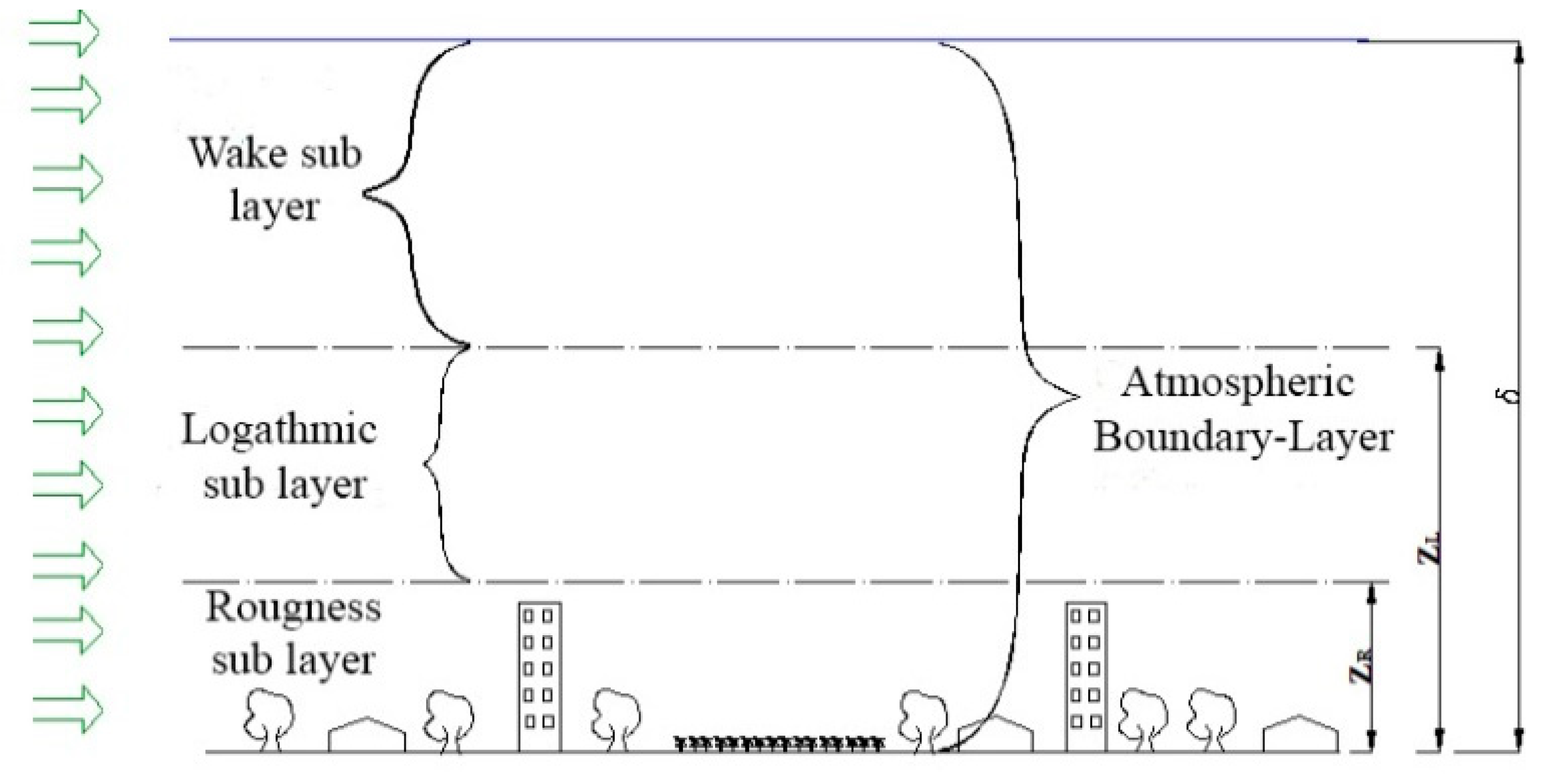
Figure 1.
Atmospheric boundary layer sublayers.
Figure 1.
Atmospheric boundary layer sublayers.
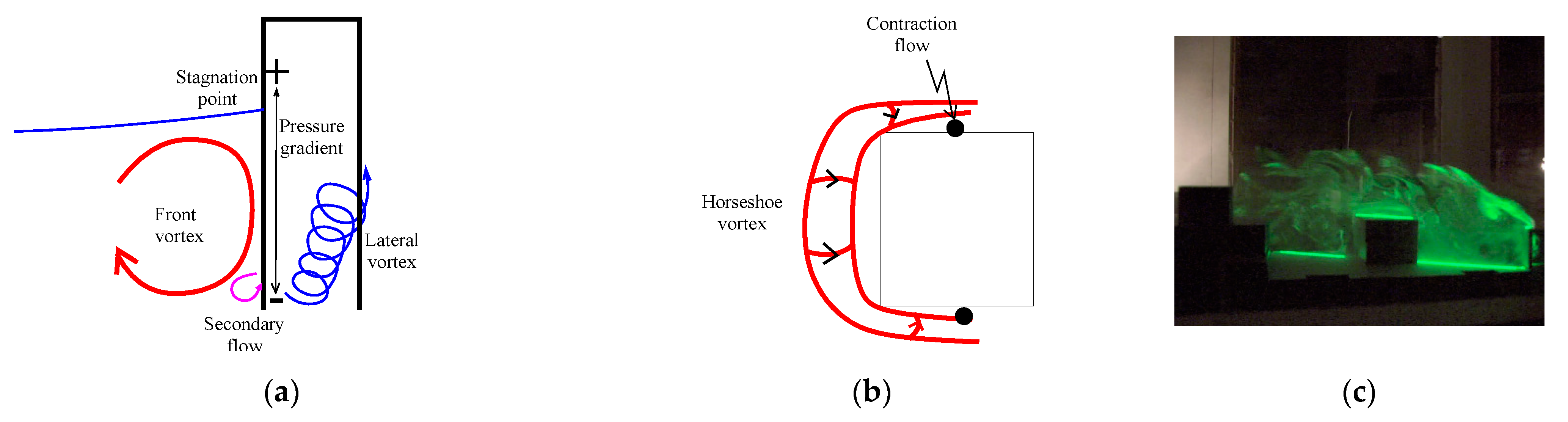
Figure 2.
Typical flows around bluff bodies: (a) the common boundary layer separation with the production of vortices and turbulence; (b) the common horse-shaped vortices developed at the base of high buildings developing strong convergence/divergence of the flow producing strong vorticity gradients; (c) the flow complexity around multiple obstacles very closed to each other as seen by a wind tunnel experiment.
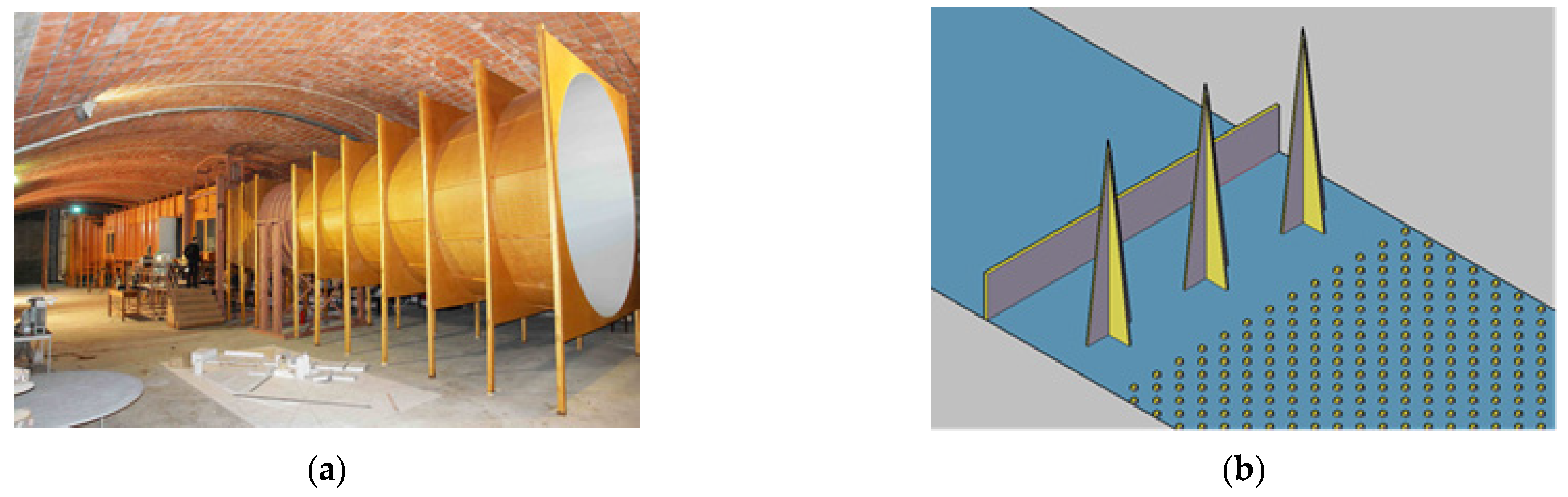
Figure 3.
(a) Wind tunnel at the School of Engineering of the Universidad de “la República” Uruguay; (b) the Standen Method for the establishment of the vertical wind profile according to roughness length and mean wind speed.
Figure 3.
(a) Wind tunnel at the School of Engineering of the Universidad de “la República” Uruguay; (b) the Standen Method for the establishment of the vertical wind profile according to roughness length and mean wind speed.
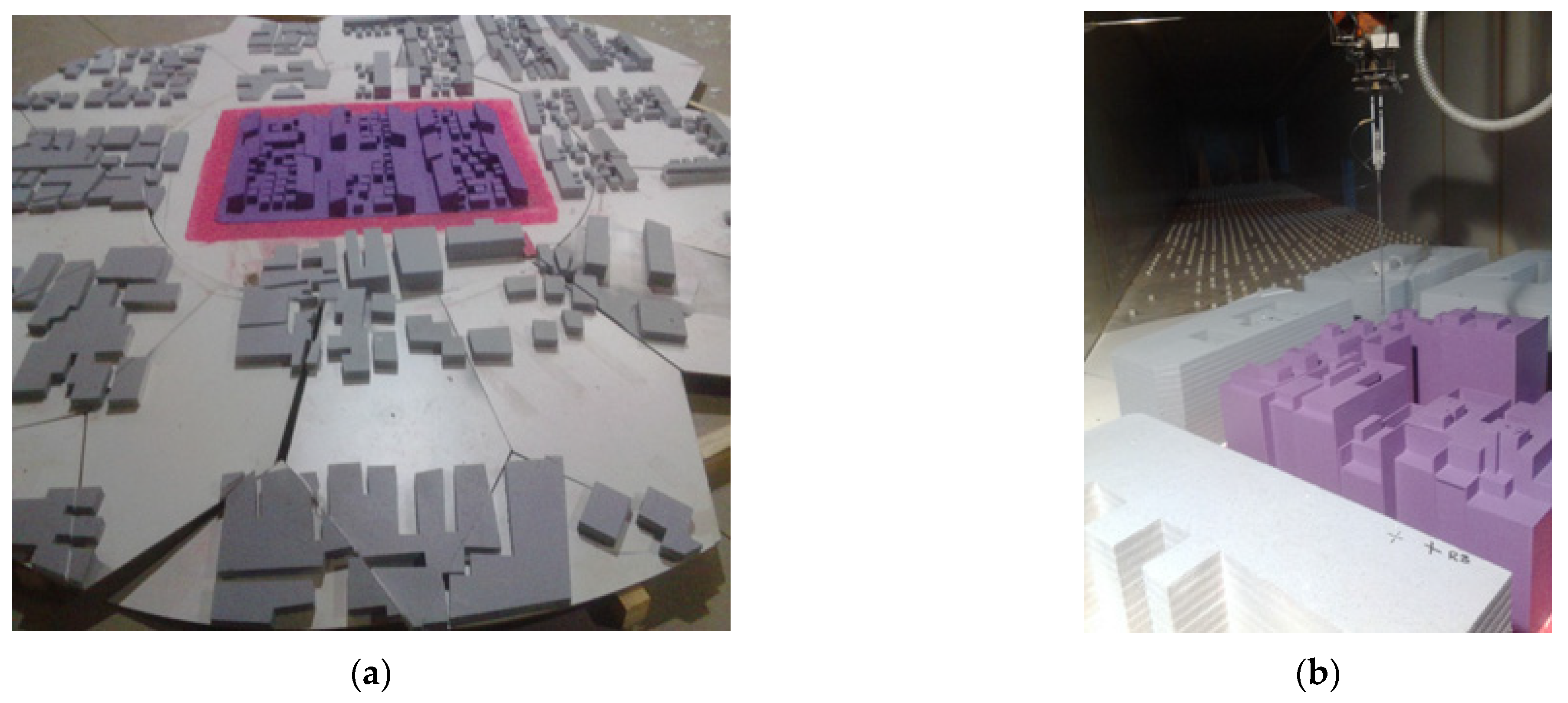
Figure 4.
(a) Urban area and surroundings model at a geometrical scale of 1/100. The purple area represents the focus urban area to be evaluated by numerical models; (b) the IFA 300 hot wire/film under operation mounted in a four-degree positioner.
Figure 4.
(a) Urban area and surroundings model at a geometrical scale of 1/100. The purple area represents the focus urban area to be evaluated by numerical models; (b) the IFA 300 hot wire/film under operation mounted in a four-degree positioner.
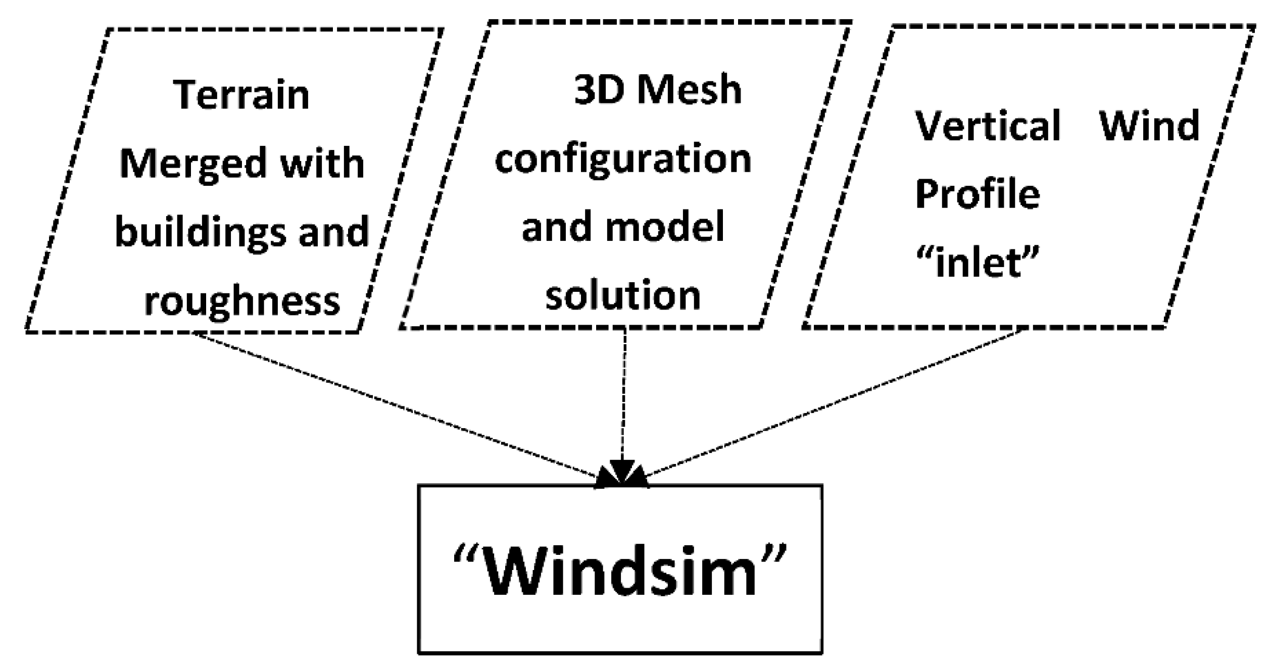
Figure 5.
Schematic workflow for performing a simulation with the WindSim model.
Figure 5.
Schematic workflow for performing a simulation with the WindSim model.
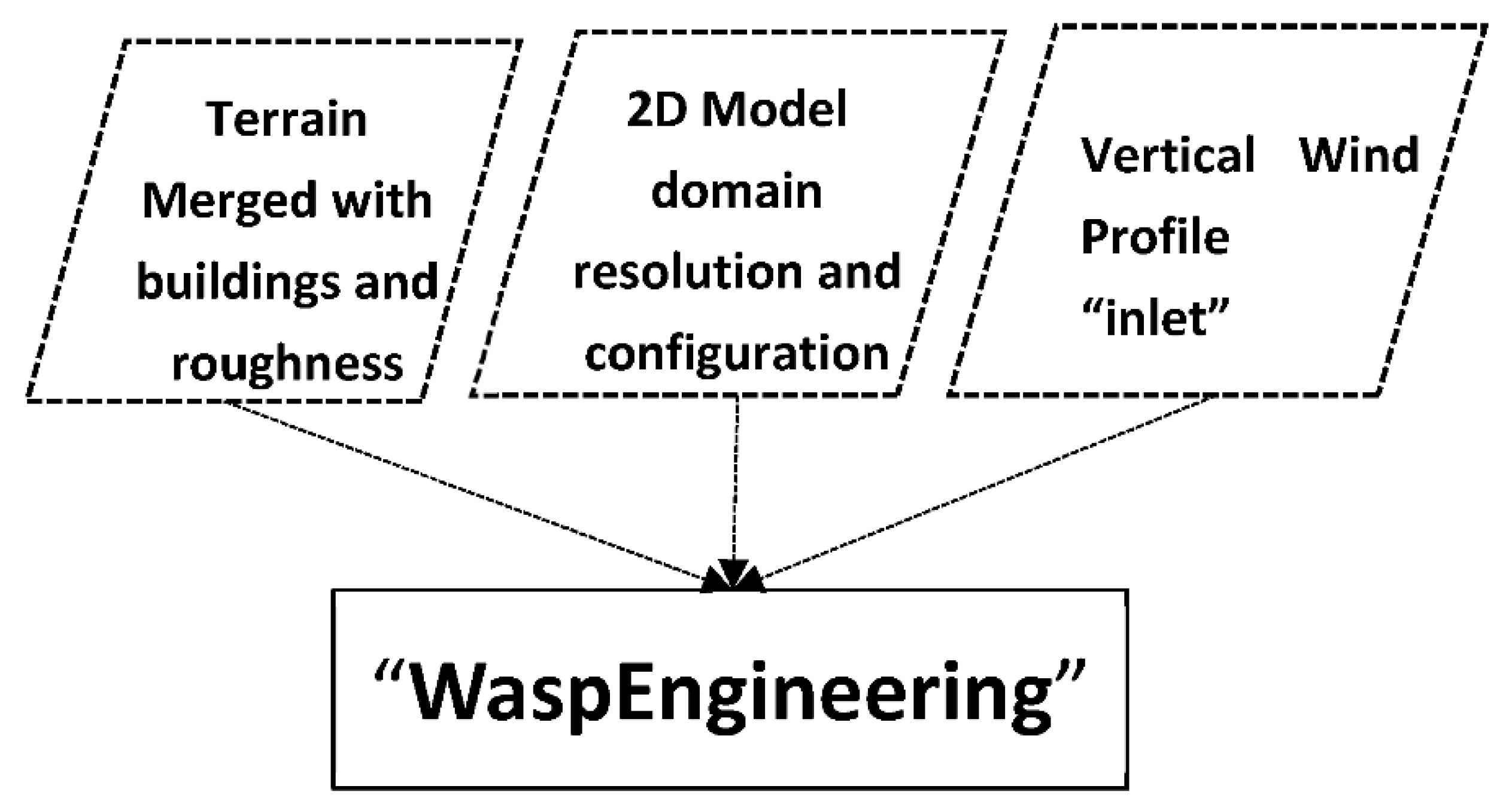
Figure 6.
Schematic workflow for performing a simulation with WAsP Engineering.
Figure 6.
Schematic workflow for performing a simulation with WAsP Engineering.
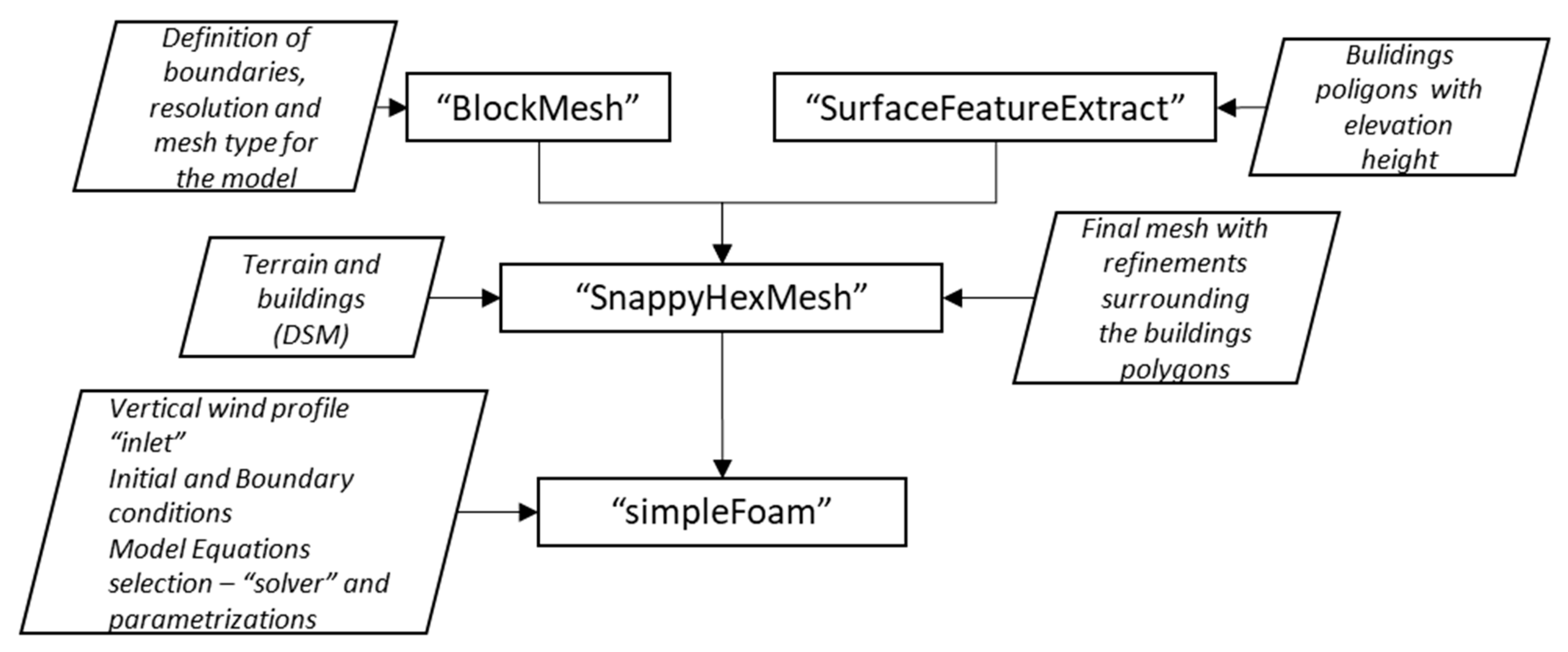
Figure 7.
Schematic workflow for performing a simulation with the OpenFOAM model.
Figure 7.
Schematic workflow for performing a simulation with the OpenFOAM model.
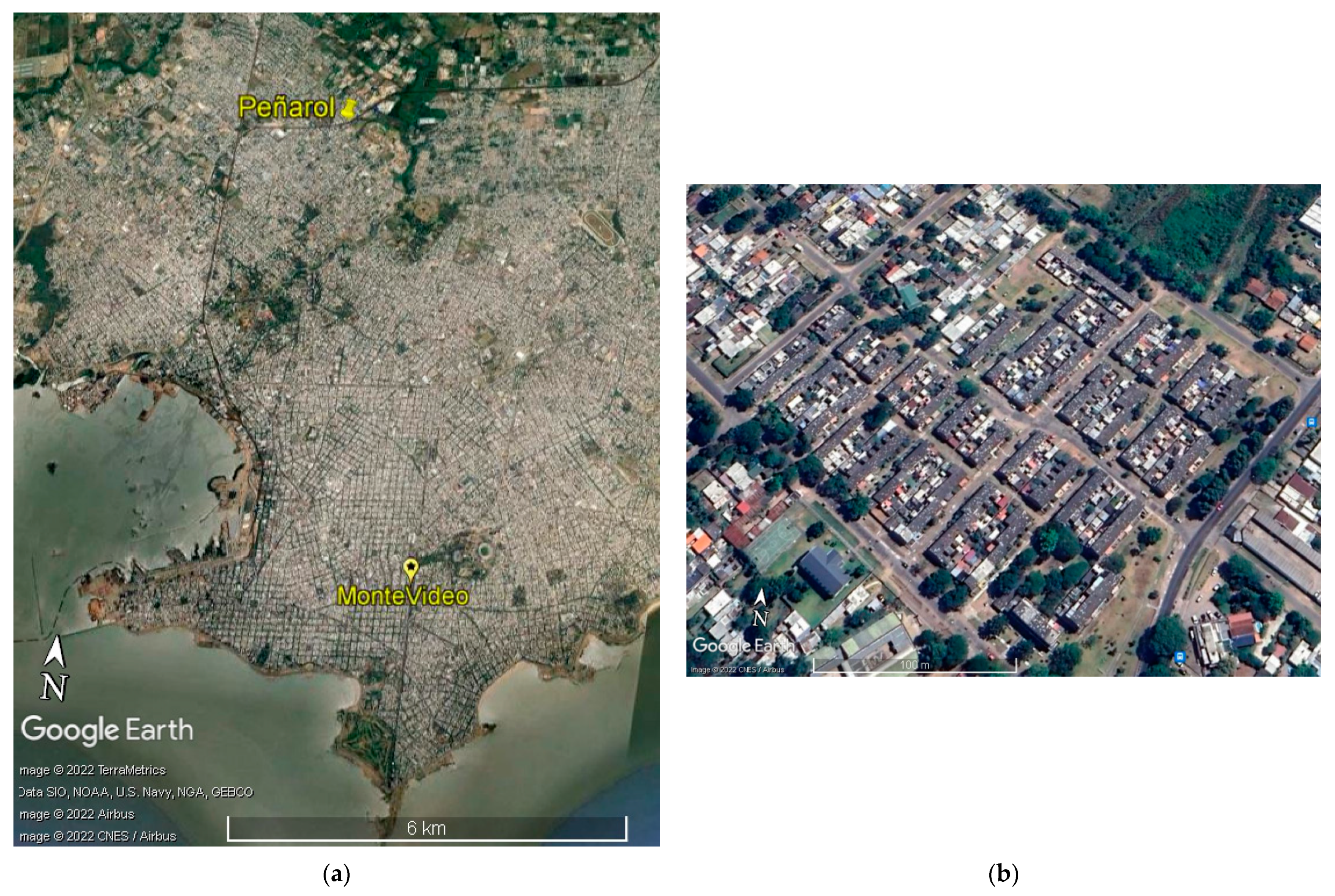
Figure 8.
(a) Montevideo City with the location of the urban area under study merged in the surroundings of the Peñarol area; (b) zoom overused area for the case study.
Figure 8.
(a) Montevideo City with the location of the urban area under study merged in the surroundings of the Peñarol area; (b) zoom overused area for the case study.
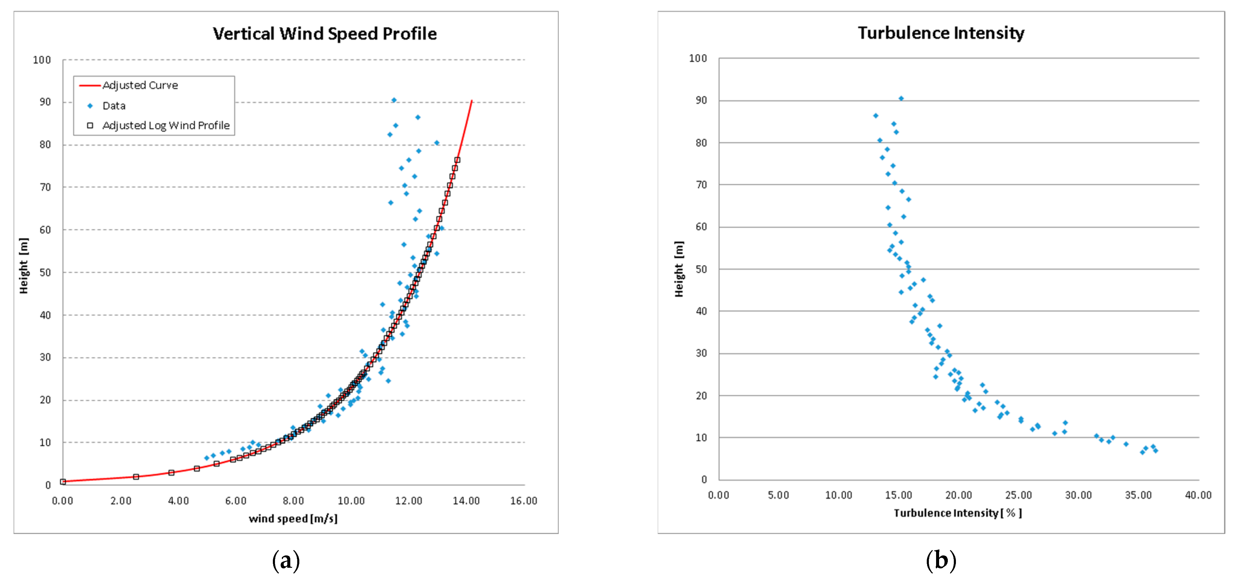
Figure 9.
(a) Estimated vertical wind profile at the surrounding urban area; (b) the turbulence intensity distribution by several reads at different heights up to scaled 90 m height.
Figure 9.
(a) Estimated vertical wind profile at the surrounding urban area; (b) the turbulence intensity distribution by several reads at different heights up to scaled 90 m height.
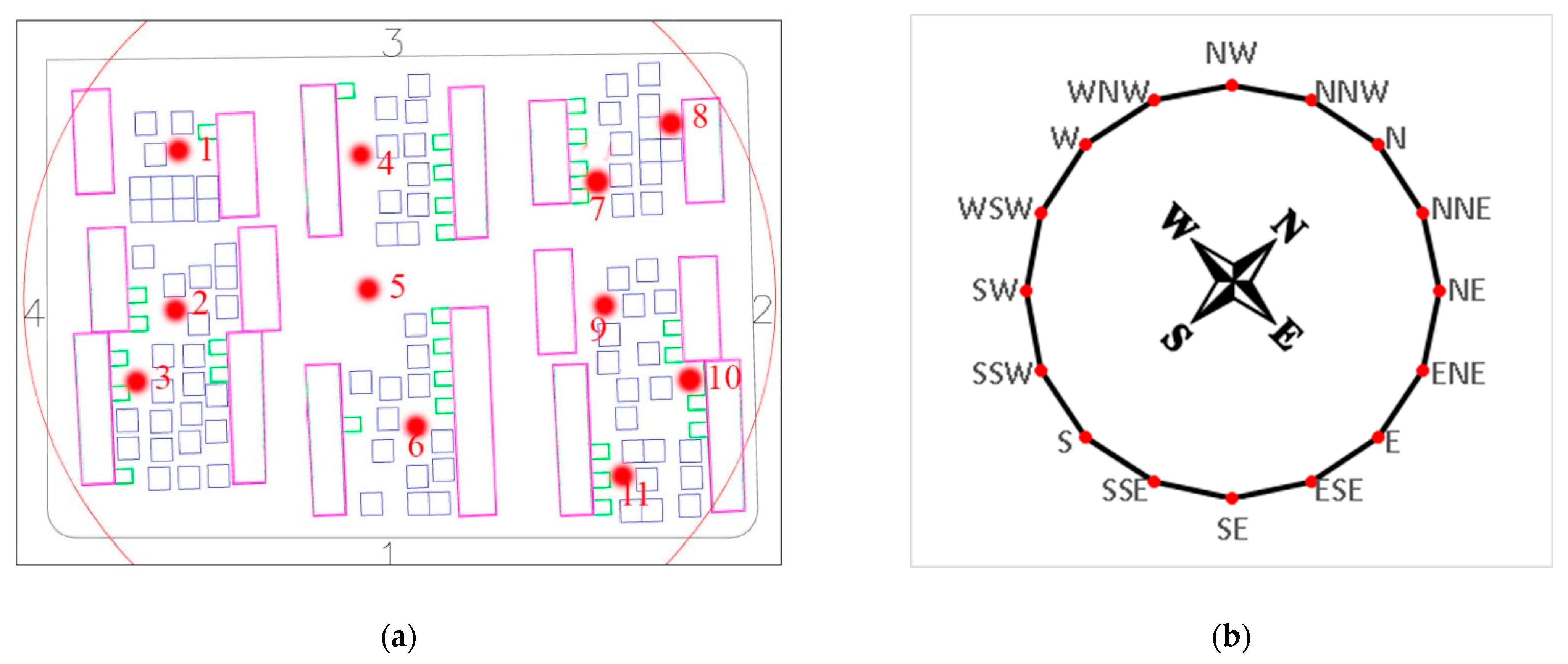
Figure 10.
(a) Location of the 11 probe points in the wind tunnel to infer the wind flow at three different heights above ground level; (b) Sixteen-degree rotating sectors (according to wind rose) for probing the data according to the projection of (a).
Figure 10.
(a) Location of the 11 probe points in the wind tunnel to infer the wind flow at three different heights above ground level; (b) Sixteen-degree rotating sectors (according to wind rose) for probing the data according to the projection of (a).
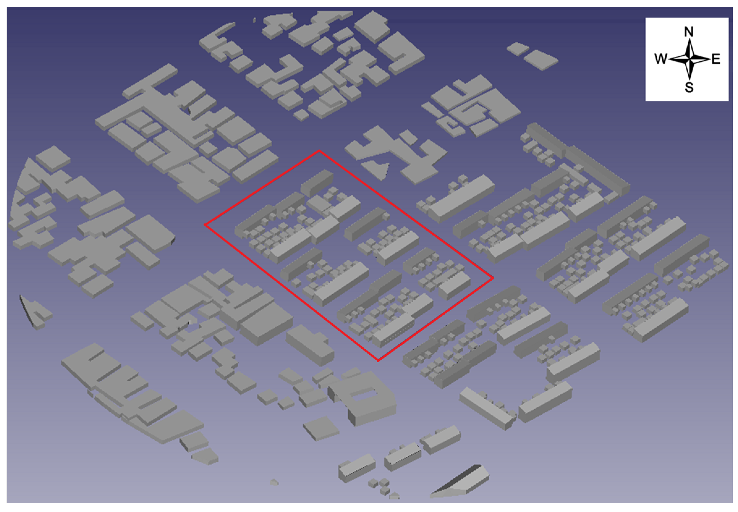
Figure 11.
Circular urban area model (red area—the focus urban area) with surroundings at a scale of 1/100 with a radius of 200 m from the midway point.
Figure 11.
Circular urban area model (red area—the focus urban area) with surroundings at a scale of 1/100 with a radius of 200 m from the midway point.
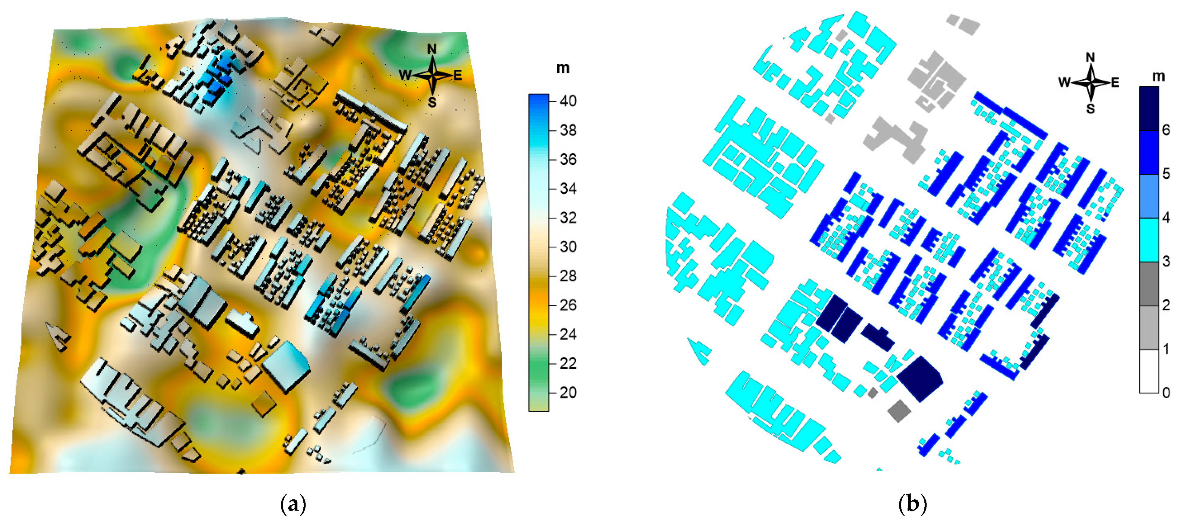
Figure 12.
(a)—Digital urban terrain model of the urban area for WAsP Engineering and WindSim models—Vertical exaggeration of 1.5×; (b) Buildings height.
Figure 12.
(a)—Digital urban terrain model of the urban area for WAsP Engineering and WindSim models—Vertical exaggeration of 1.5×; (b) Buildings height.
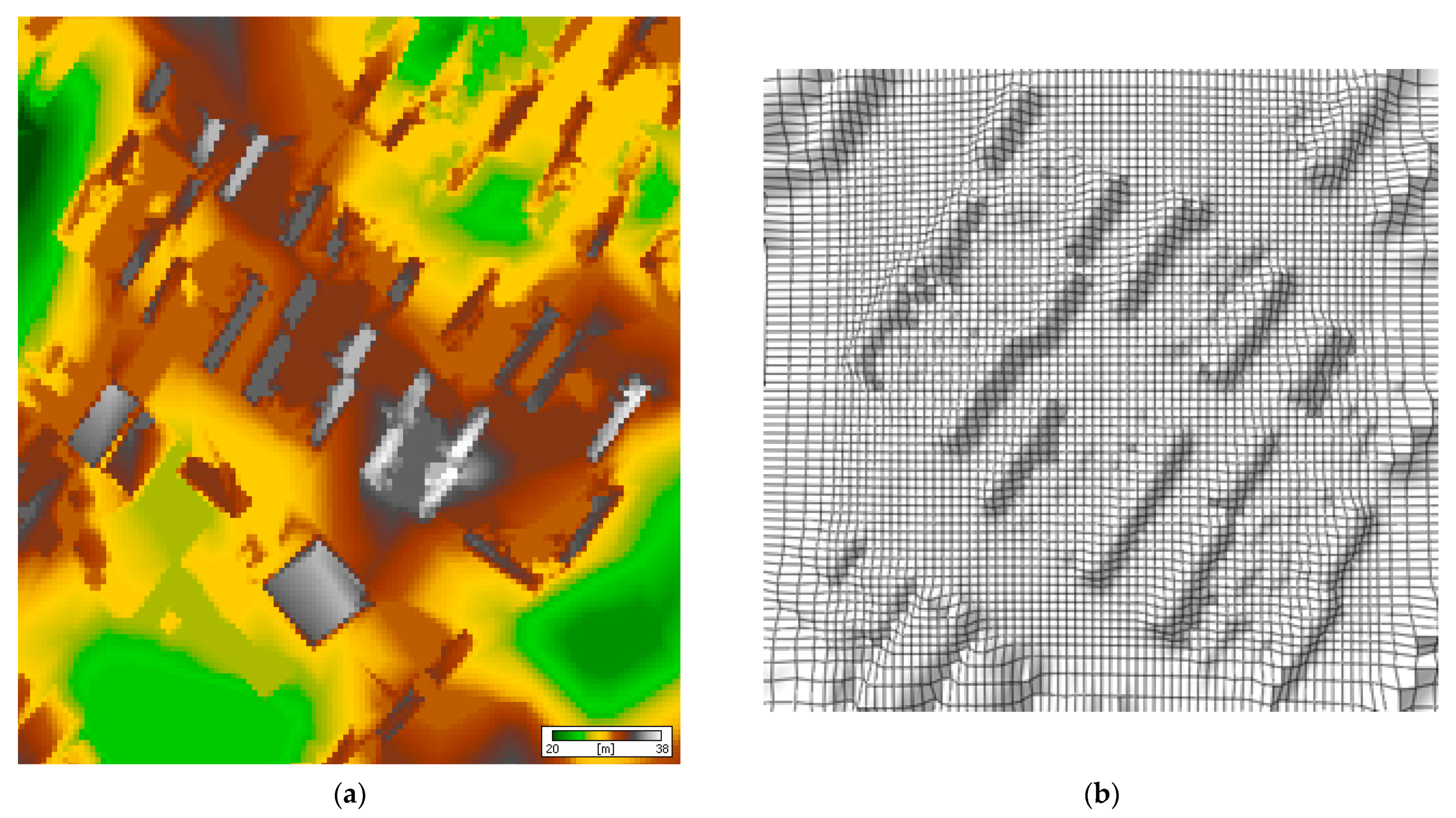
Figure 13.
(a)—Digital urban terrain model at 0.5 m × 0.5 m spatial resolution computed by WAsP Engineering; (b) Regular nested mesh generated by WindSim model for the central urban area with 2 m × 2 m spatial resolution.
Figure 13.
(a)—Digital urban terrain model at 0.5 m × 0.5 m spatial resolution computed by WAsP Engineering; (b) Regular nested mesh generated by WindSim model for the central urban area with 2 m × 2 m spatial resolution.
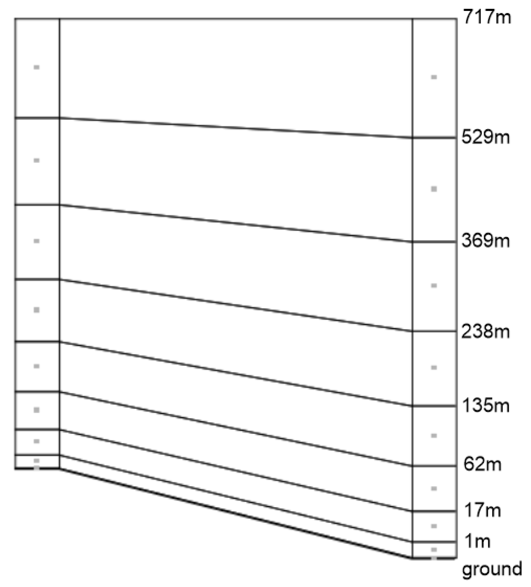
Figure 14.
Schematic representation of the 3D vertical structure refined mesh generated by WindSim model. Eight vertical levels were considered to meet the convergence criteria of the CFD solver.
Figure 14.
Schematic representation of the 3D vertical structure refined mesh generated by WindSim model. Eight vertical levels were considered to meet the convergence criteria of the CFD solver.
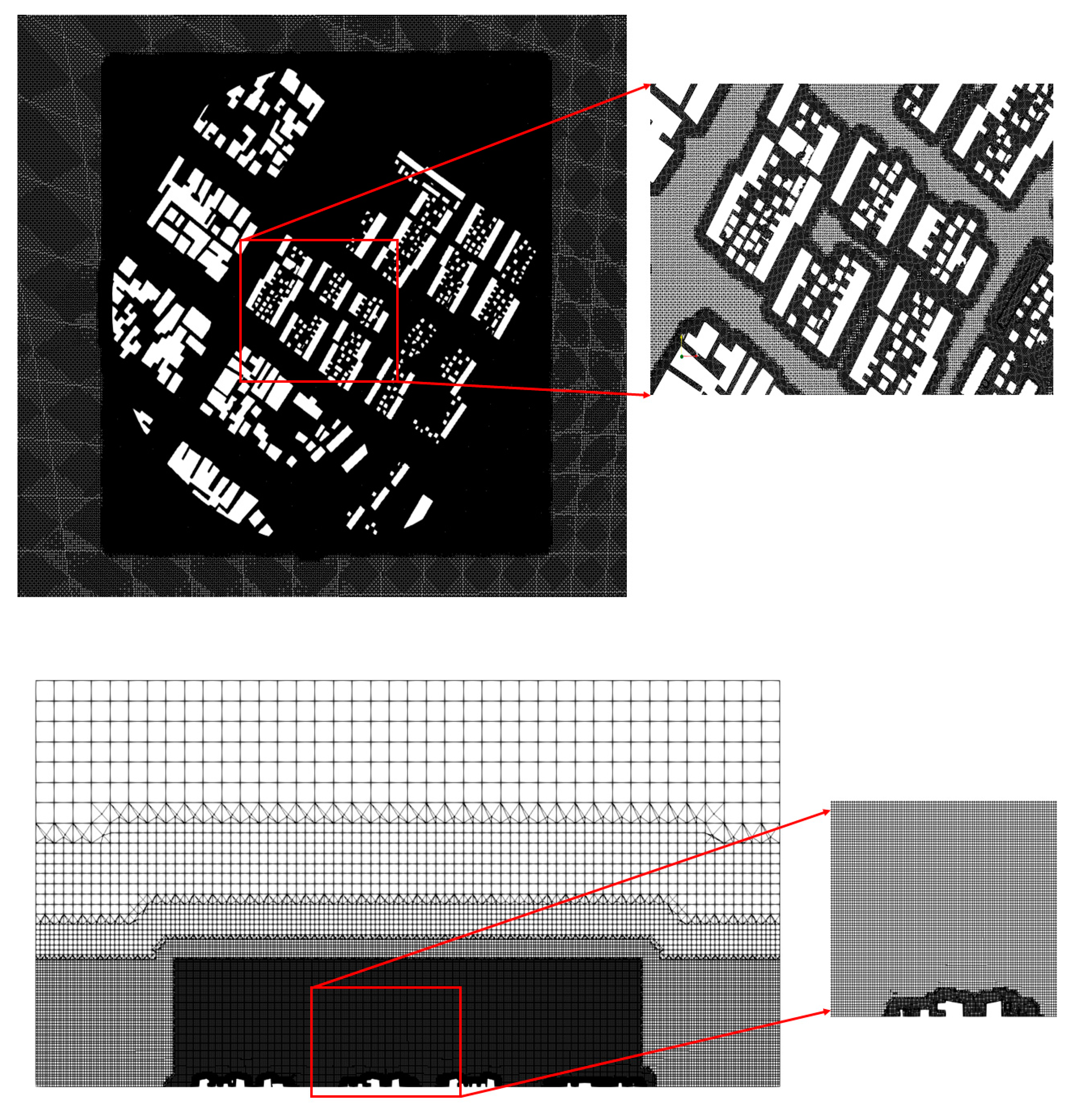
Figure 15.
Mesh used for the OpenFOAM computational domain, detailing the zones used for different element sizes near the building’s walls.
Figure 15.
Mesh used for the OpenFOAM computational domain, detailing the zones used for different element sizes near the building’s walls.
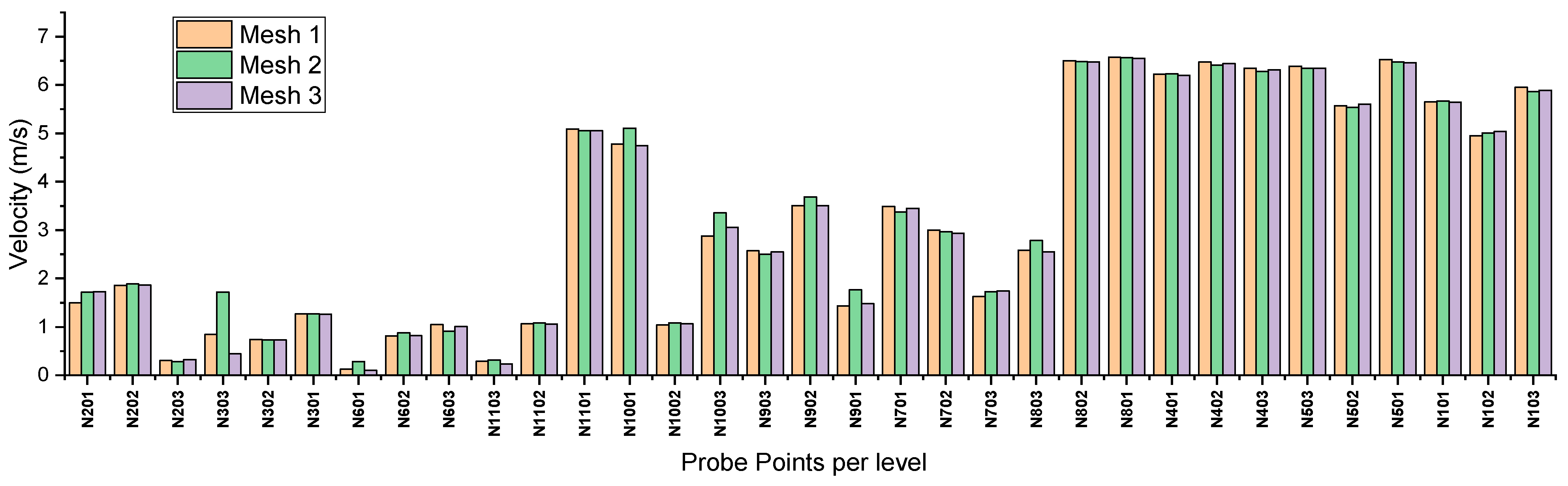
Figure 16.
Mesh independence study considering three different meshes for the OpenFOAM computational domain. Velocity in validation points. Hypothetical vertical wind profile considered.
Figure 16.
Mesh independence study considering three different meshes for the OpenFOAM computational domain. Velocity in validation points. Hypothetical vertical wind profile considered.
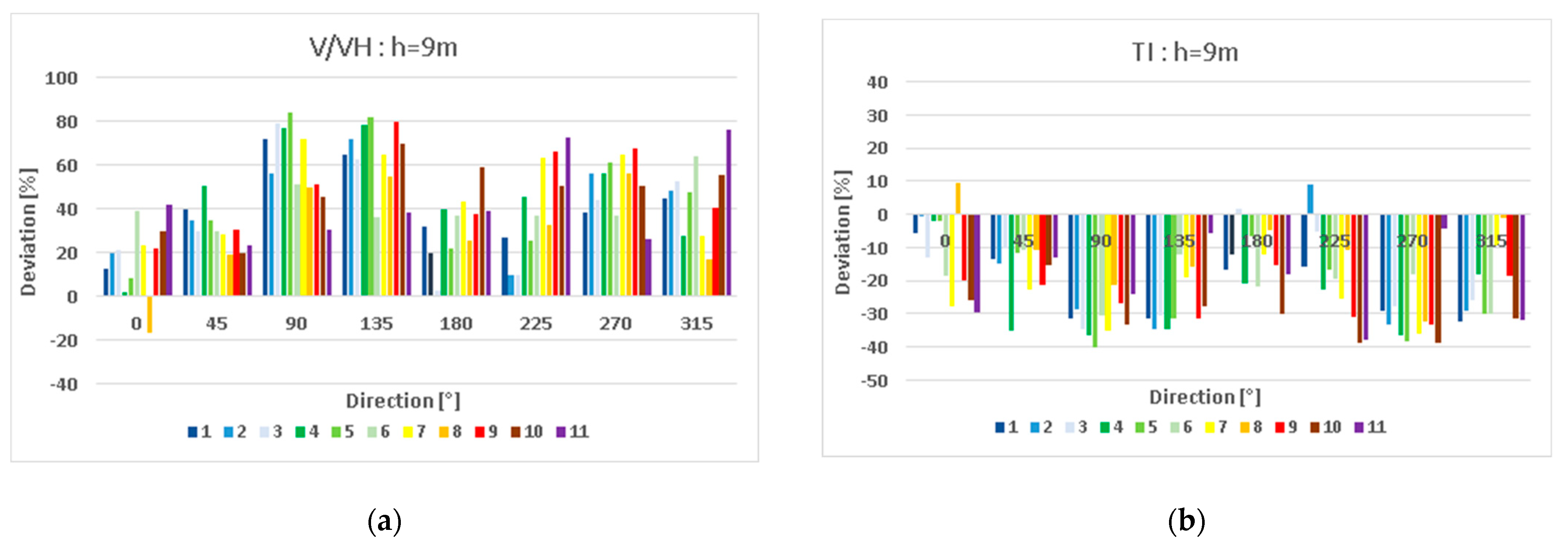
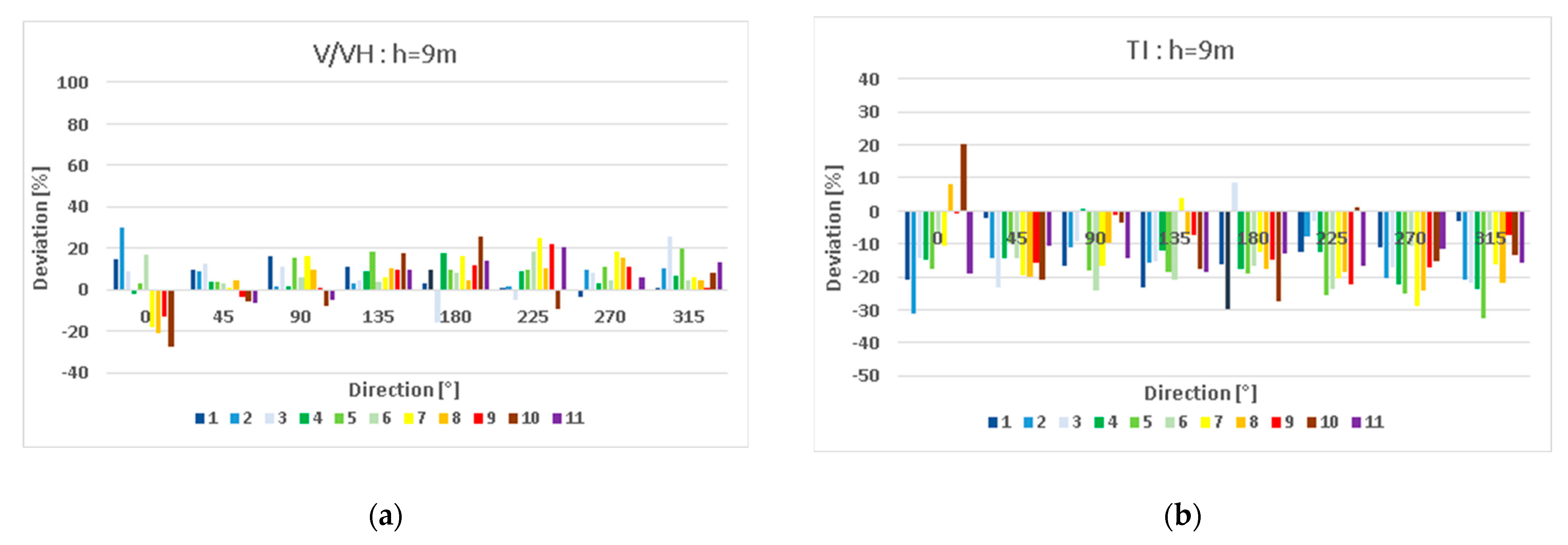
Figure 17.
Mean absolute deviations of the wind (a) and turbulence intensity (b) per direction for the 11 probe validation points at height h = 9 m with WAsP Engineering.
Figure 17.
Mean absolute deviations of the wind (a) and turbulence intensity (b) per direction for the 11 probe validation points at height h = 9 m with WAsP Engineering.
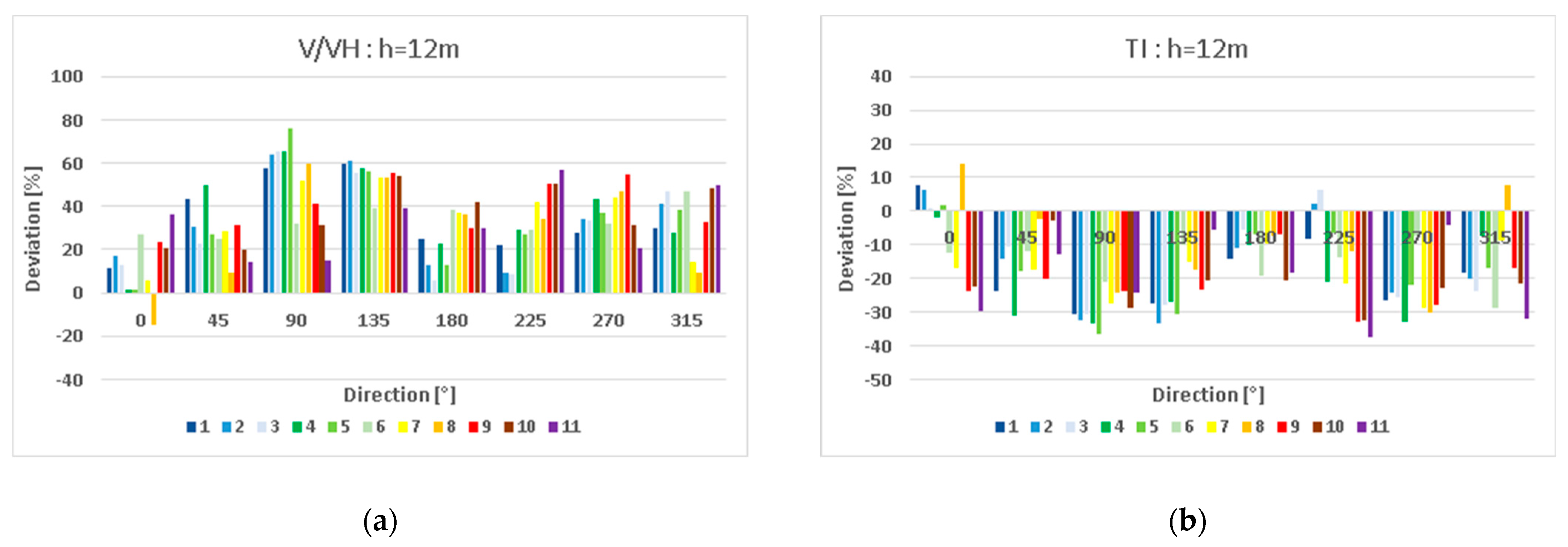
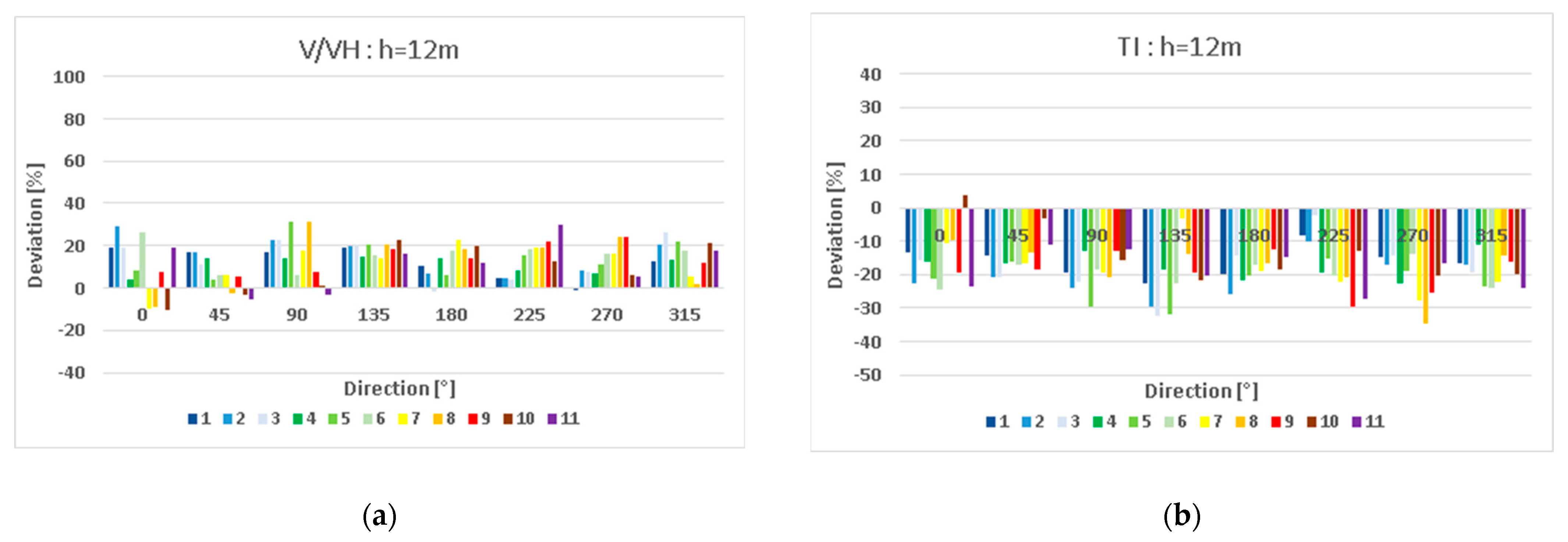
Figure 18.
Mean absolute deviations of the wind (a) and turbulence intensity (b) per direction for the 11 probe validation points at height h = 12 m with WAsP Engineering.
Figure 18.
Mean absolute deviations of the wind (a) and turbulence intensity (b) per direction for the 11 probe validation points at height h = 12 m with WAsP Engineering.
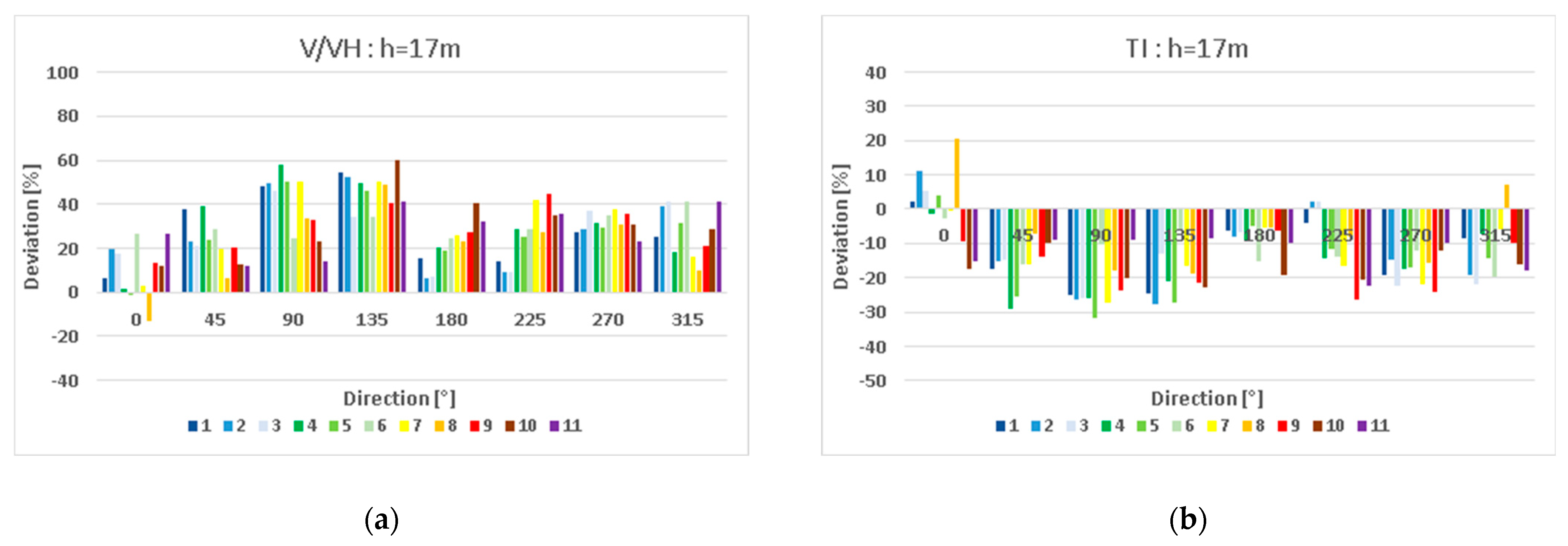
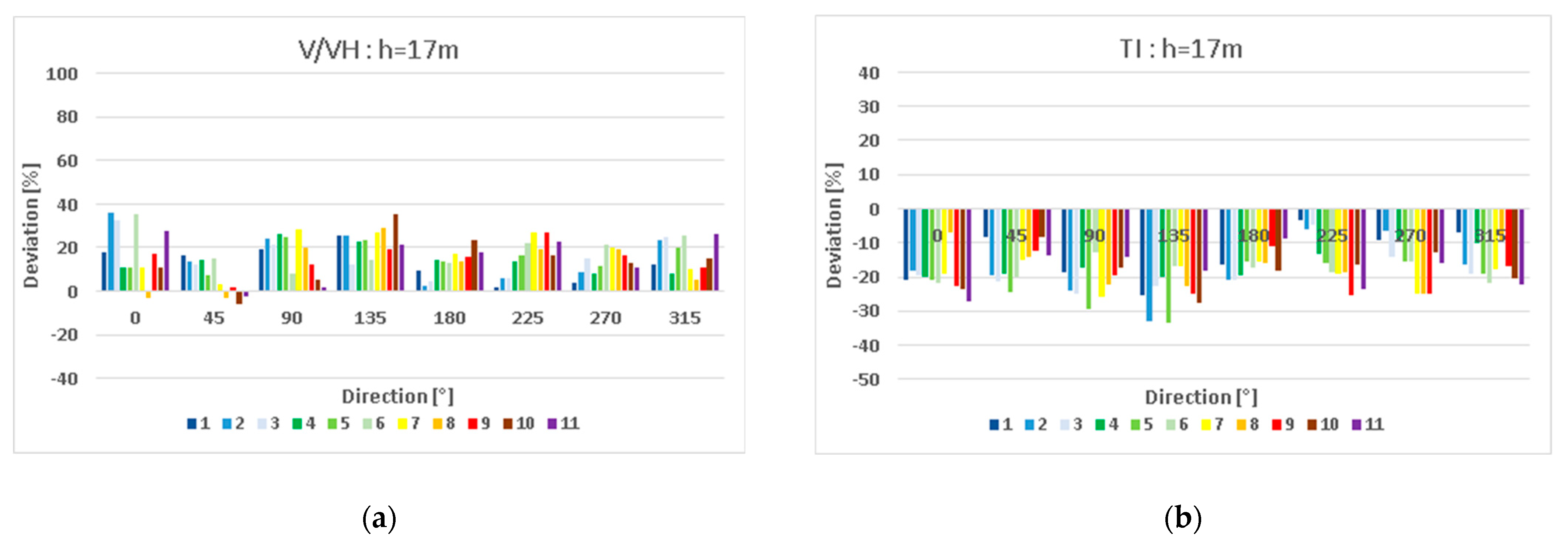
Figure 19.
Mean absolute deviations of the wind (a) and turbulence intensity (b) per direction for the 11 probe validation points at height h = 17 m with WAsP Engineering.
Figure 19.
Mean absolute deviations of the wind (a) and turbulence intensity (b) per direction for the 11 probe validation points at height h = 17 m with WAsP Engineering.
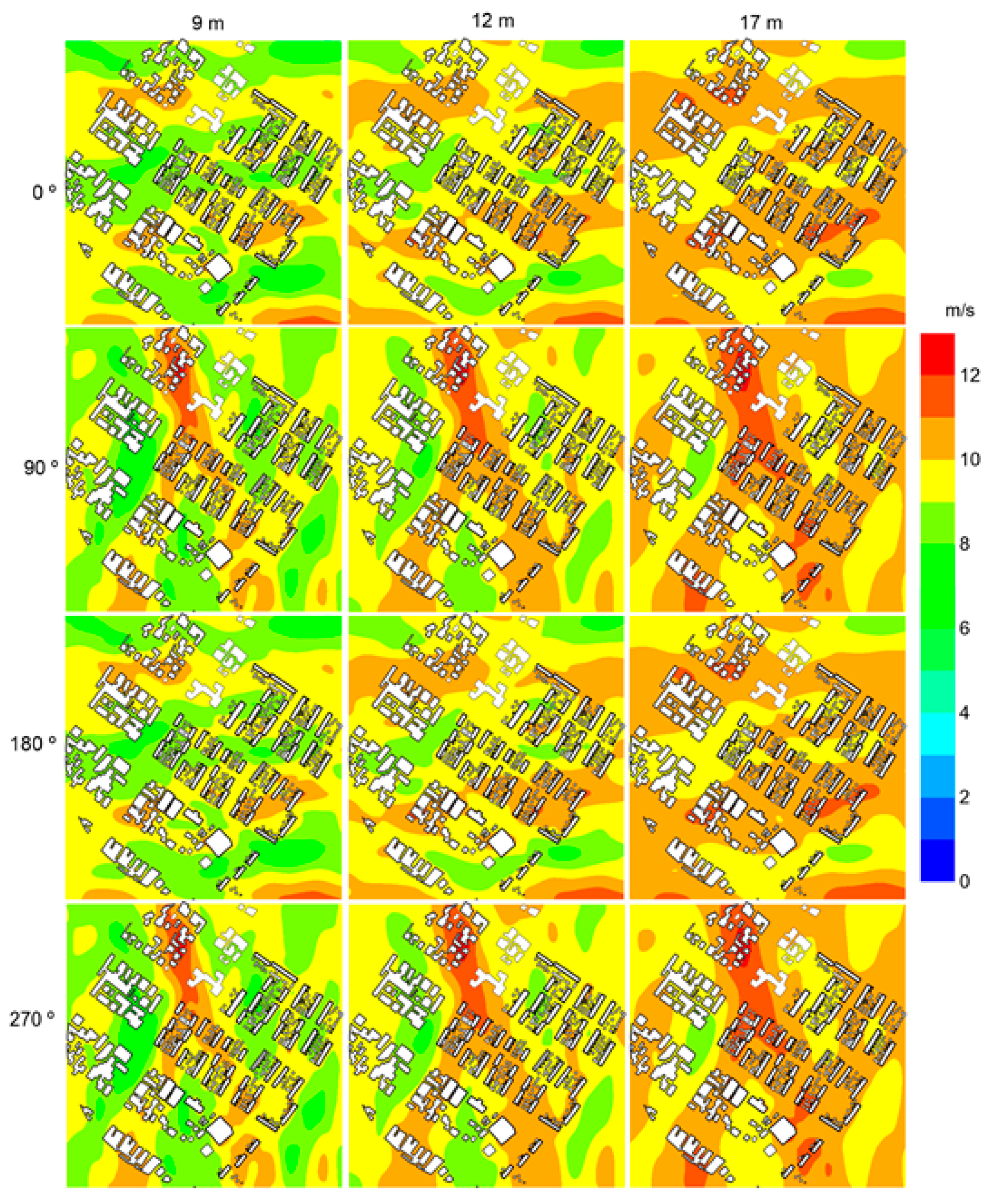
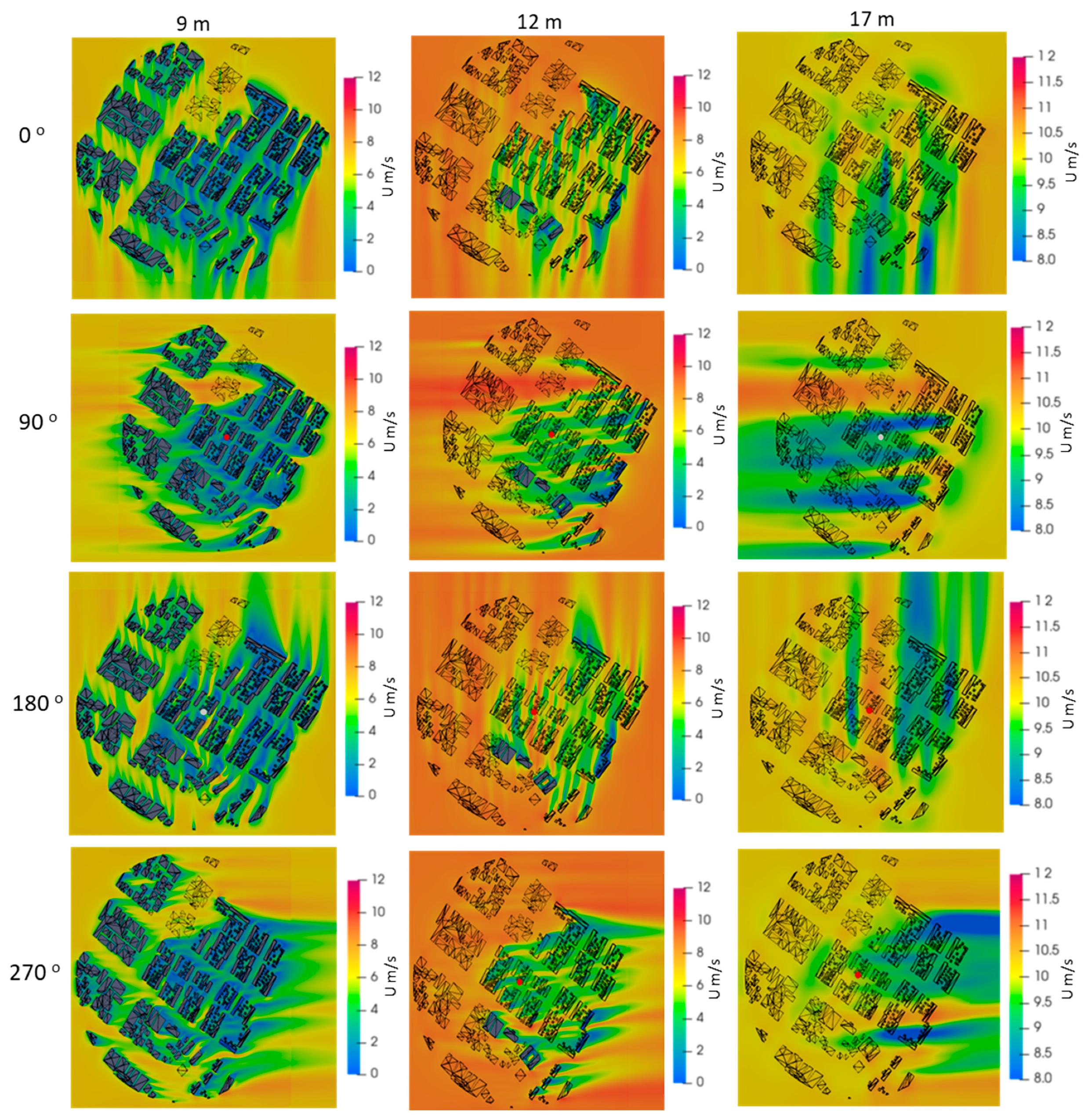
Figure 20.
Mean wind speed estimates obtained by the WAsP Engineering model for three heights (9 m, 12 m, and 17 m) and four wind sectors rose (0°, 90°, 180°, and 270°).
Figure 20.
Mean wind speed estimates obtained by the WAsP Engineering model for three heights (9 m, 12 m, and 17 m) and four wind sectors rose (0°, 90°, 180°, and 270°).
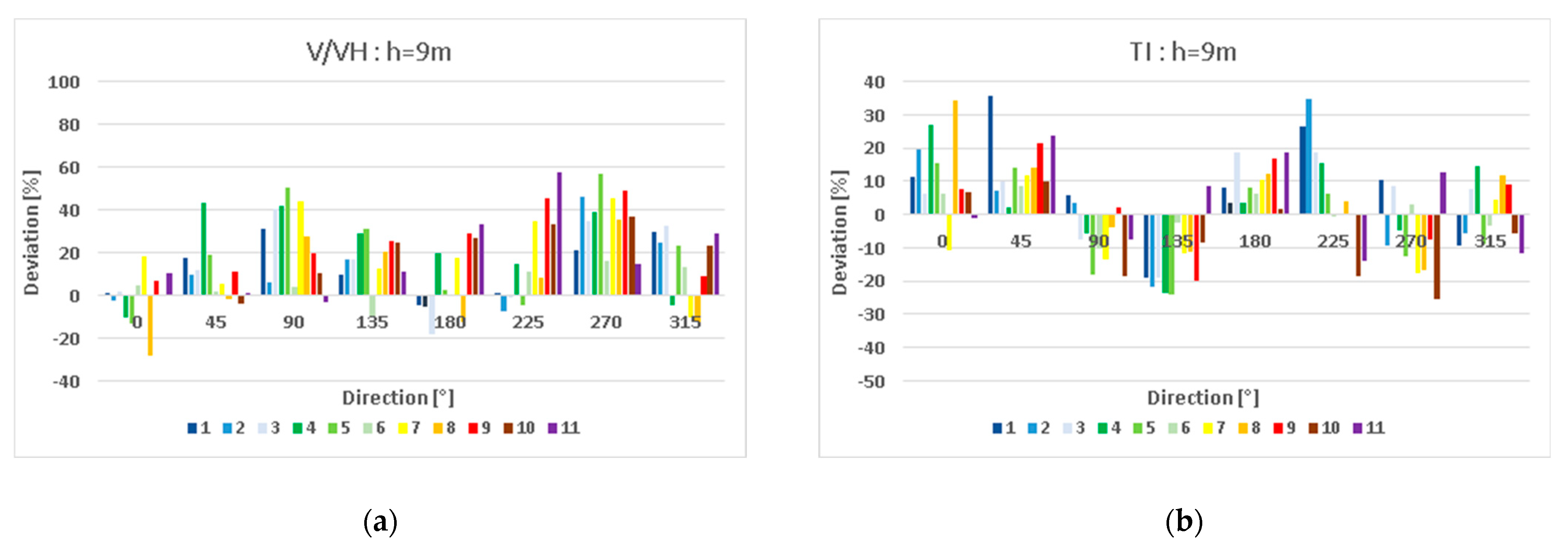
Figure 21.
Mean absolute deviations of the wind (a) and turbulence intensity (b) per direction for the 11 probe validation points at height h = 9 m with Windsim.
Figure 21.
Mean absolute deviations of the wind (a) and turbulence intensity (b) per direction for the 11 probe validation points at height h = 9 m with Windsim.
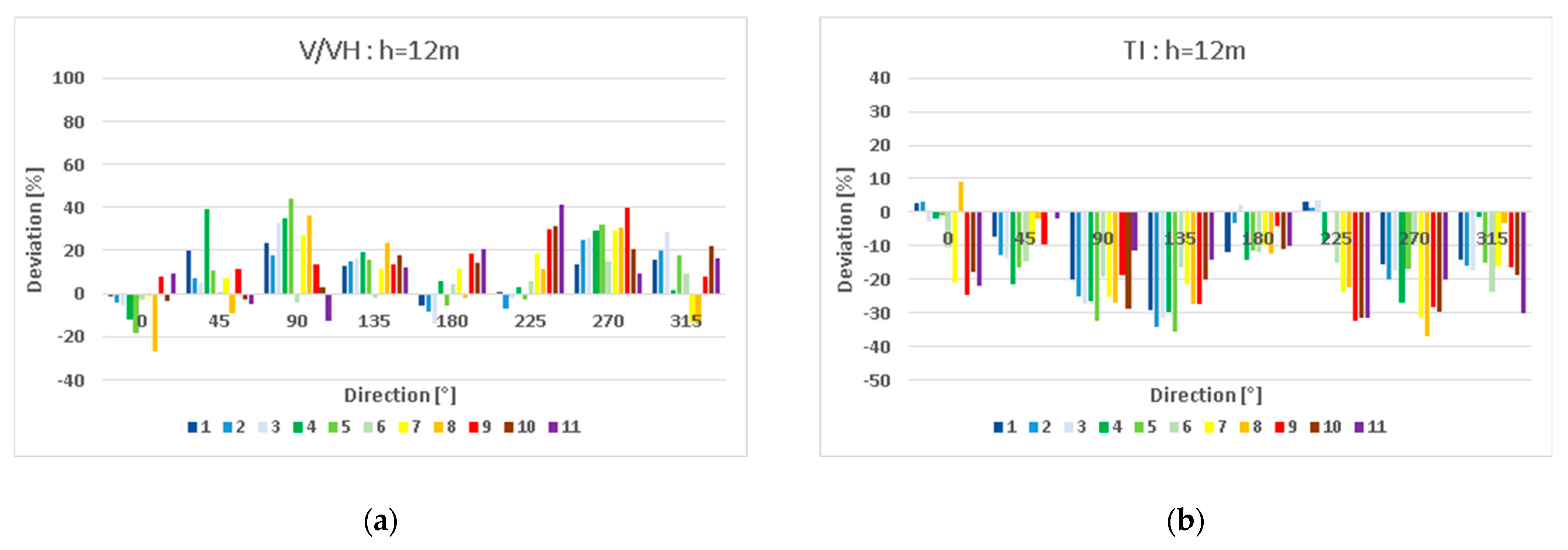
Figure 22.
Mean absolute deviations of the wind (a) and turbulence intensity (b) per direction for the 11 probe validation points at height h = 12 m with Windsim.
Figure 22.
Mean absolute deviations of the wind (a) and turbulence intensity (b) per direction for the 11 probe validation points at height h = 12 m with Windsim.
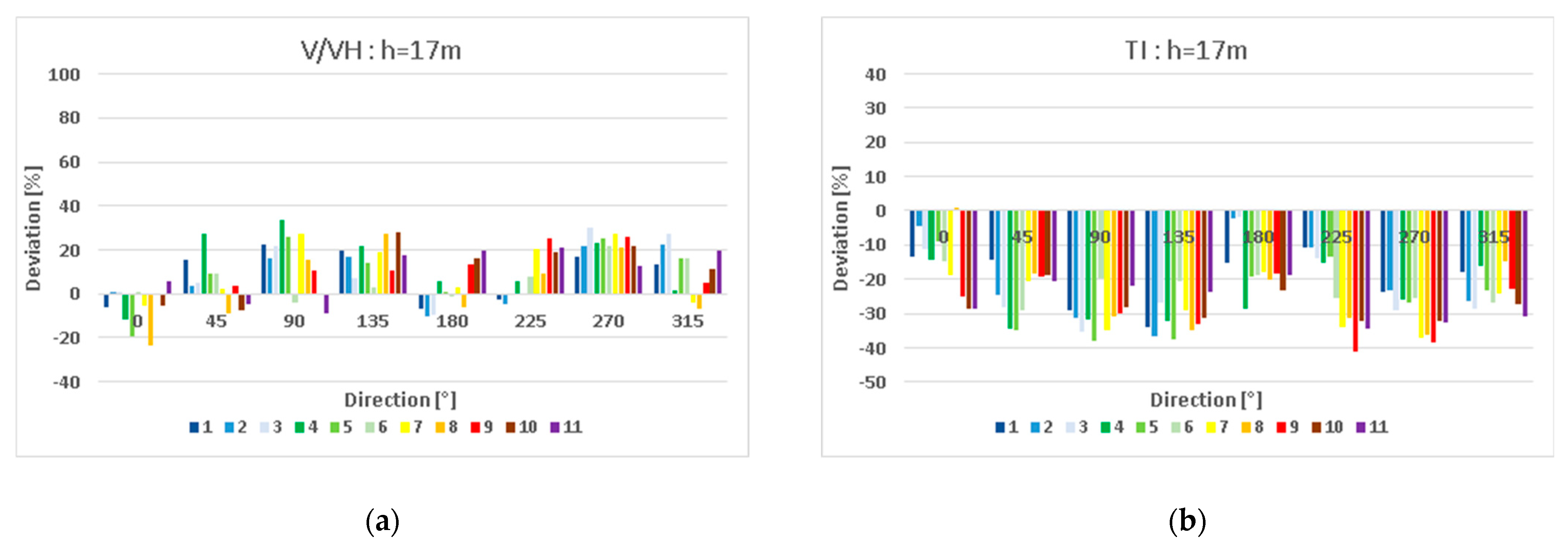
Figure 23.
Mean absolute deviations of the wind (a) and turbulence intensity (b) per direction for the 11 probe validation points at height h = 17 m with WindSim.
Figure 23.
Mean absolute deviations of the wind (a) and turbulence intensity (b) per direction for the 11 probe validation points at height h = 17 m with WindSim.
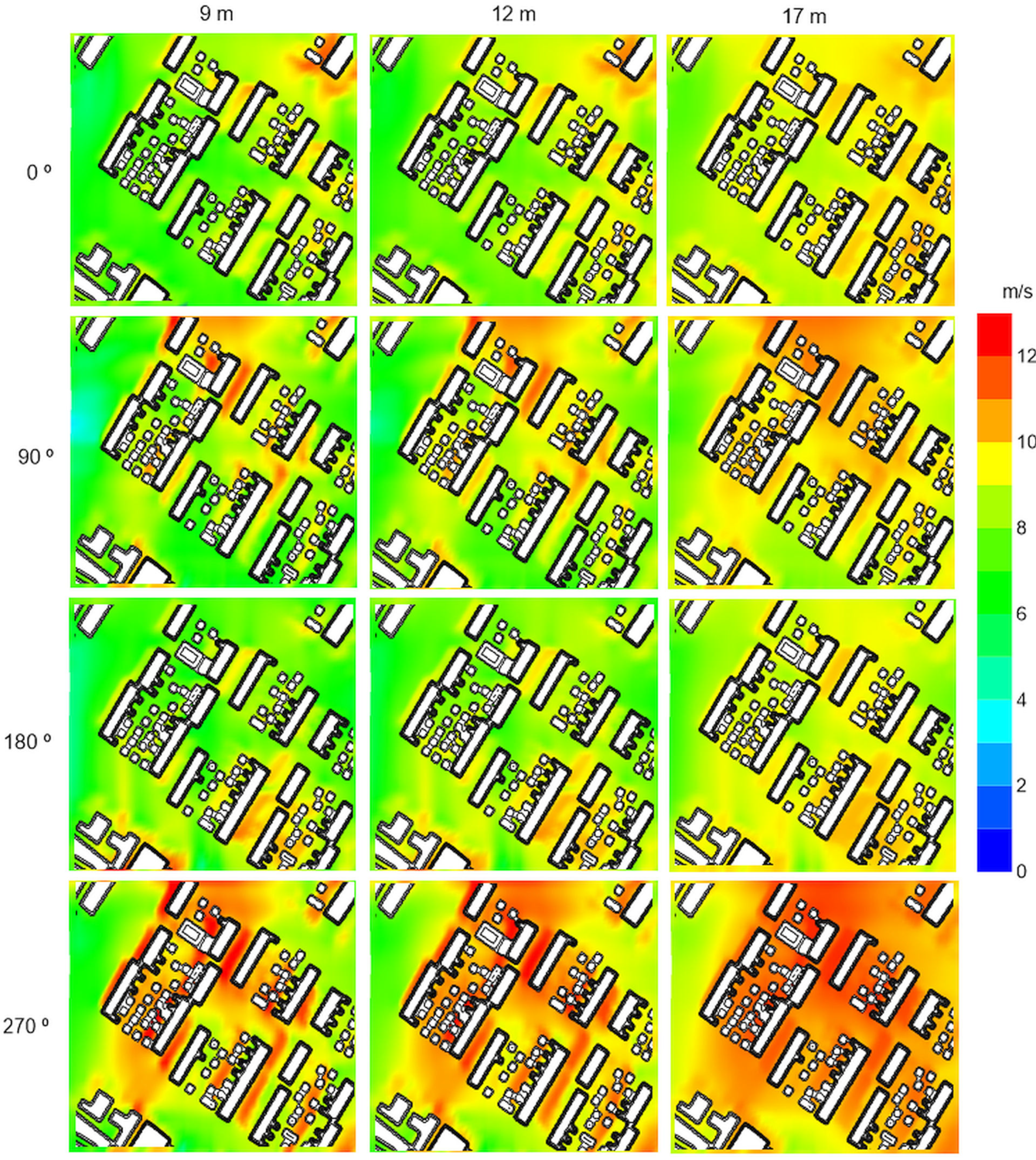
Figure 24.
Mean wind speed estimates obtained by the WindSim model for three heights (9 m, 12 m, and 17 m) and four wind sectors rose (0°, 90°, 180°, and 270°).
Figure 24.
Mean wind speed estimates obtained by the WindSim model for three heights (9 m, 12 m, and 17 m) and four wind sectors rose (0°, 90°, 180°, and 270°).
Figure 25.
Mean absolute deviations of the wind (a) and turbulence intensity (b) per direction for the 11 probe validation points at height h = 9 m with OpenFOAM.
Figure 25.
Mean absolute deviations of the wind (a) and turbulence intensity (b) per direction for the 11 probe validation points at height h = 9 m with OpenFOAM.
Figure 26.
Mean absolute deviations of the wind (a) and turbulence intensity (b) per direction for the 11 probe validation points at height h = 12 m with OpenFOAM.
Figure 26.
Mean absolute deviations of the wind (a) and turbulence intensity (b) per direction for the 11 probe validation points at height h = 12 m with OpenFOAM.
Figure 27.
Mean absolute deviations of the wind (a) and turbulence intensity (b) per direction for the 11 probe validation points at height h = 17 m with OpenFOAM.
Figure 27.
Mean absolute deviations of the wind (a) and turbulence intensity (b) per direction for the 11 probe validation points at height h = 17 m with OpenFOAM.
Figure 28.
Mean wind speed estimates obtained by the OpenFOAM CFD model for three heights (9 m, 12 m, and 17 m) and four wind sectors rose (0°, 90°, 180°, and 270°).
Figure 28.
Mean wind speed estimates obtained by the OpenFOAM CFD model for three heights (9 m, 12 m, and 17 m) and four wind sectors rose (0°, 90°, 180°, and 270°).
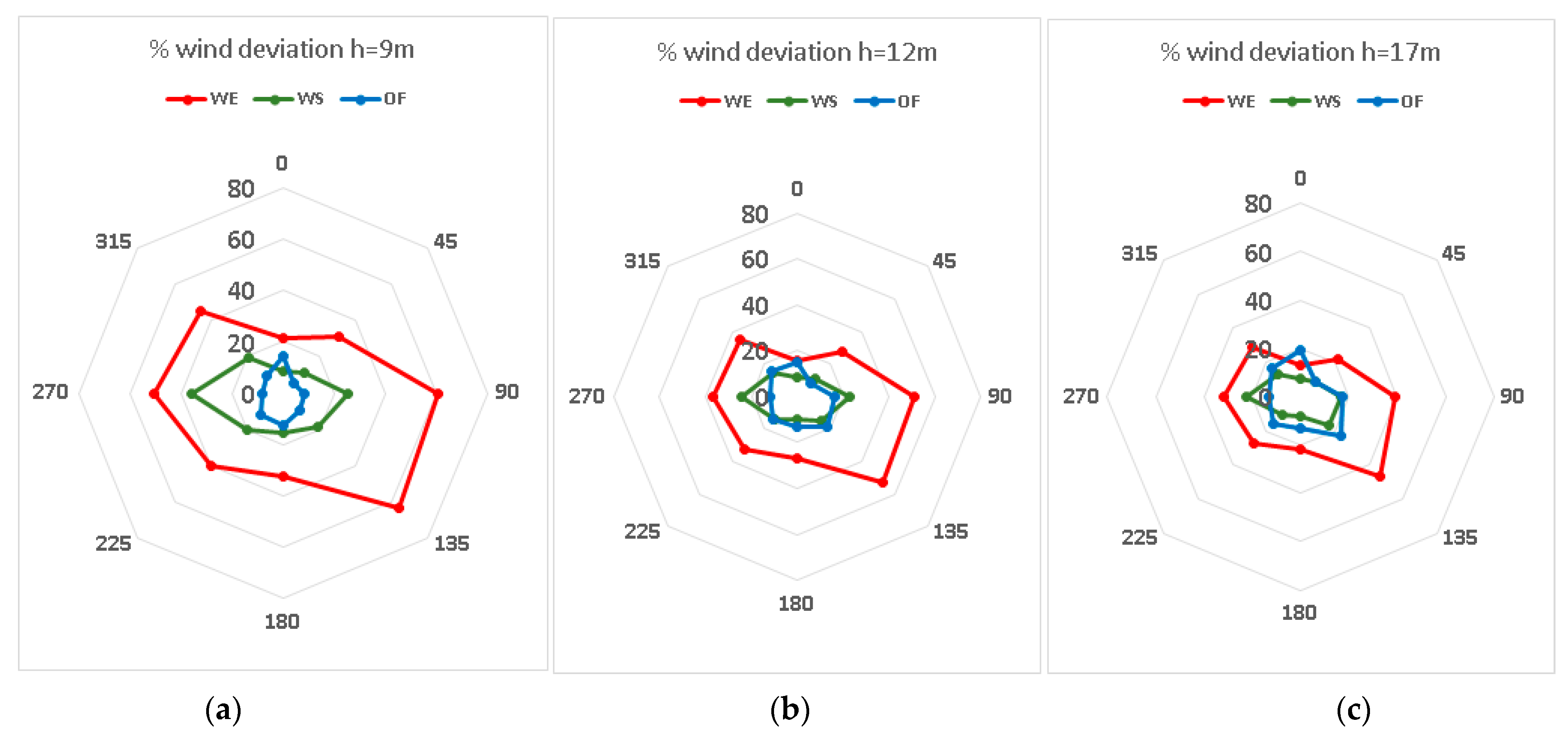
Figure 29.
Overall mean wind speed absolute deviation per points 1, 2, 3 and per height (a)—9 m, (b)—12 m, and (c)—17 m above ground.
Figure 29.
Overall mean wind speed absolute deviation per points 1, 2, 3 and per height (a)—9 m, (b)—12 m, and (c)—17 m above ground.
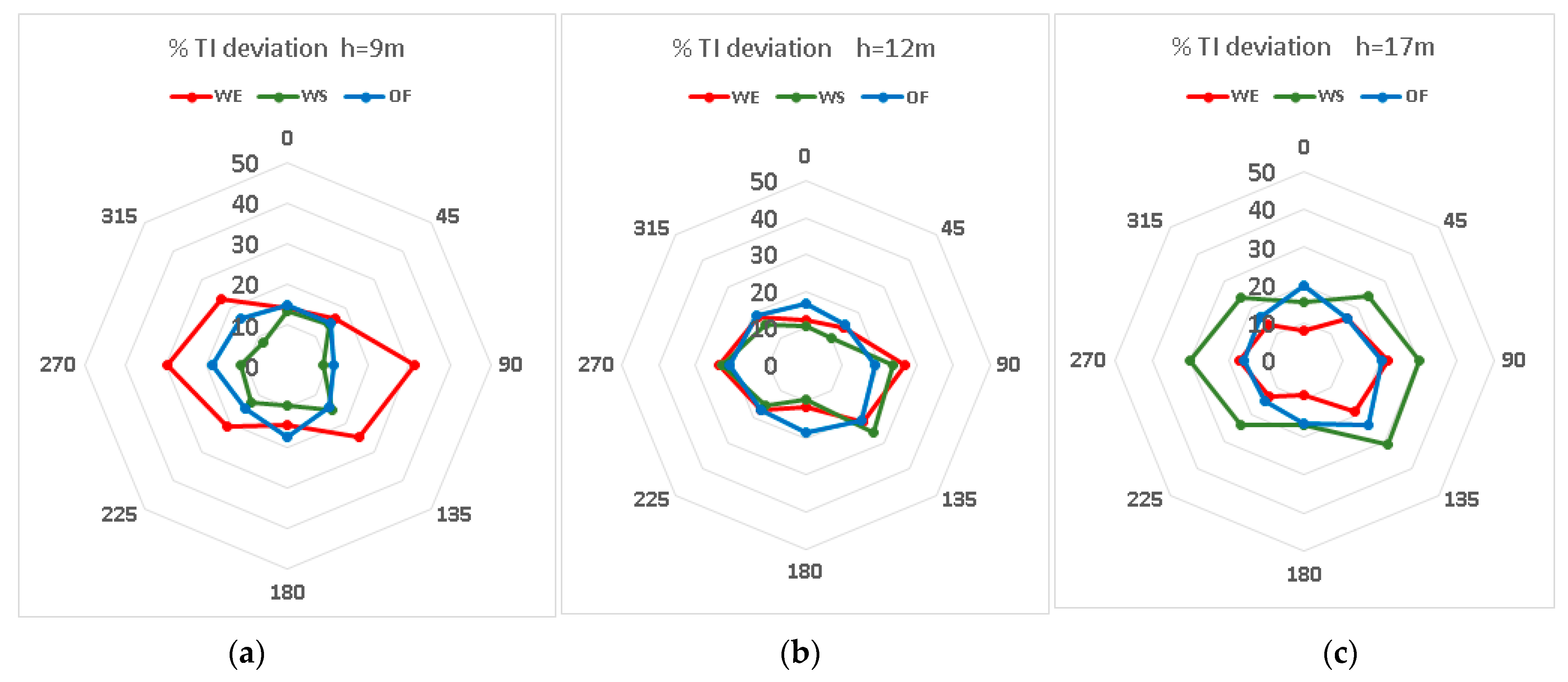
Figure 30.
Overall mean turbulence intensity absolute deviation per points 1, 2, 3 and per height (a)—9 m, (b)—12 m, and (c)—17 m above ground.
Figure 30.
Overall mean turbulence intensity absolute deviation per points 1, 2, 3 and per height (a)—9 m, (b)—12 m, and (c)—17 m above ground.
Table 1.
Initial and boundary conditions imposed for the WAsP Engineering model.
Table 1.
Initial and boundary conditions imposed for the WAsP Engineering model.
| Model Version | WAsP Engineering v. 2.0 |
|---|
| Initial Conditions | Urban digital terrain model Top of boundary layer: 200 m height above ground Spatial resolution: 0.5 m × 0.5 m Roughness length: Z0 = 0.87 m (dense occupation);
|
| Boundary Conditions | |
Table 2.
Initial and boundary conditions imposed for the Windsim model.
Table 2.
Initial and boundary conditions imposed for the Windsim model.
| Model Version | Windsim v. 6.0 |
|---|
| Initial Conditions | Urban digital terrain model Top of boundary layer: 800 m height above ground Refined orthogonal 3D grid: 2 m × 2 m Roughness Height: Z0 = 0.87 m (dense occupation) Height distribution factor: 0.01 Ratio additive length to resolution: 0.01 Smoothing Gaussian model:
|
| Boundary Conditions | Low height for boundary layer: 200m Speed at low height for boundary layer: 13 m/s Top boundary condition: Fixed pressure Vertical wind profile:
|
| Calculation Parameters | Solver: GCV Number of iterations: 200 Convergence criteria: 0.005 Potential temperature: Disregard temperature Air density: 1.225 kg/m3 Turbulence model: modified k-ε Height of reduced wind database: 200 m
|
Table 3.
Initial and boundary conditions imposed for the OpenFOAM model.
Table 3.
Initial and boundary conditions imposed for the OpenFOAM model.
| Model Version | OpenFOAM v. 2012 |
|---|
| Initial Conditions | STL model of the urban area Top of boundary layer: 300 m height above ground Minimum grid size: 0.5m Aerodynamic roughness length: Z0 = 0.087 m
|
| Boundary Conditions | Speed above boundary layer height: 13 m/s Top and sides boundaries: Slip Inlet condition: atmBoundaryLayerInletVelocity Vref = 12.95 m/s Zref = 60 m Z0 = uniform = 0.087 m Zground = 0
|
| Calculation Parameters | Solver: simpleFoam Number of iterations: 5000 Convergence criteria: 0.0001 Potential temperature: Disregard temperature Air density: 1.225 kg/m3 Turbulence model: standard k-ε
|
Table 4.
Wind tunnel results per direction per point (1 to 11) and per height. V/VH is the ratio between velocity (V) and velocity at the top of the boundary Layer (VH); TI is the turbulence intensity. The height above ground is given by .1, .2, and .3, meaning 9 m, 12 m, and 17 m, respectively.
Table 4.
Wind tunnel results per direction per point (1 to 11) and per height. V/VH is the ratio between velocity (V) and velocity at the top of the boundary Layer (VH); TI is the turbulence intensity. The height above ground is given by .1, .2, and .3, meaning 9 m, 12 m, and 17 m, respectively.
| Point | N-0° | NE-45° | E-90° | SE-135°º | S-180° | SW-225° | W-270° | NW-315° |
|---|
| V/VH | T.I | V/VH | T.I | V/VH | T.I | V/VH | T.I | V/VH | T.I | V/VH | T.I | V/VH | T.I | V/VH | T.I |
|---|
| [%] | [%] | [%] | [%] | [%] | [%] | [%] | [%] | [%] | [%] | [%] | [%] | [%] | [%] | [%] | [%] |
|---|
| 1.1 | 0.61 | 23 | 0.58 | 19 | 0.49 | 24 | 0.44 | 29 | 0.52 | 25 | 0.64 | 20 | 0.61 | 22 | 0.5 | 28 |
| 1.2 | 0.65 | 19 | 0.58 | 21 | 0.55 | 23 | 0.48 | 26 | 0.58 | 23 | 0.68 | 18 | 0.68 | 21 | 0.59 | 22 |
| 1.3 | 0.72 | 19 | 0.62 | 19 | 0.60 | 21 | 0.52 | 24 | 0.66 | 20 | 0.75 | 17 | 0.70 | 19 | 0.64 | 19 |
| 2.1 | 0.56 | 23 | 0.52 | 24 | 0.50 | 26 | 0.44 | 30 | 0.56 | 25 | 0.64 | 19 | 0.50 | 26 | 0.51 | 26 |
| 2.2 | 0.61 | 20 | 0.57 | 22 | 0.50 | 26 | 0.49 | 28 | 0.63 | 23 | 0.68 | 19 | 0.61 | 22 | 0.56 | 22 |
| 2.3 | 0.63 | 18 | 0.64 | 21 | 0.57 | 23 | 0.54 | 25 | 0.71 | 21 | 0.72 | 18 | 0.66 | 19 | 0.59 | 21 |
| 3.1 | 0.55 | 26 | 0.55 | 22 | 0.45 | 27 | 0.47 | 28 | 0.65 | 22 | 0.65 | 21 | 0.56 | 23 | 0.5 | 24 |
| 3.2 | 0.63 | 21 | 0.61 | 21 | 0.50 | 25 | 0.51 | 26 | 0.67 | 22 | 0.69 | 18 | 0.62 | 22 | 0.54 | 23 |
| 3.3 | 0.64 | 19 | 0.65 | 21 | 0.58 | 23 | 0.61 | 21 | 0.70 | 21 | 0.72 | 18 | 0.62 | 21 | 0.58 | 22 |
| 4.1 | 0.70 | 21 | 0.54 | 25 | 0.46 | 27 | 0.4 | 31 | 0.51 | 25 | 0.56 | 22 | 0.52 | 26 | 0.56 | 24 |
| 4.2 | 0.74 | 20 | 0.56 | 23 | 0.51 | 25 | 0.48 | 26 | 0.61 | 21 | 0.65 | 21 | 0.59 | 24 | 0.59 | 20 |
| 4.3 | 0.77 | 19 | 0.62 | 22 | 0.55 | 22 | 0.53 | 23 | 0.65 | 20 | 0.67 | 19 | 0.66 | 19 | 0.67 | 19 |
| 5.1 | 0.61 | 24 | 0.54 | 22 | 0.42 | 31 | 0.39 | 31 | 0.54 | 24 | 0.58 | 24 | 0.48 | 29 | 0.48 | 29 |
| 5.2 | 0.70 | 21 | 0.61 | 22 | 0.46 | 28 | 0.48 | 29 | 0.63 | 22 | 0.61 | 20 | 0.59 | 22 | 0.54 | 23 |
| 5.3 | 0.77 | 19 | 0.66 | 23 | 0.56 | 25 | 0.54 | 26 | 0.64 | 20 | 0.65 | 20 | 0.65 | 20 | 0.6 | 21 |
| 6.1 | 0.52 | 25 | 0.56 | 22 | 0.48 | 29 | 0.53 | 24 | 0.53 | 25 | 0.53 | 25 | 0.53 | 24 | 0.44 | 28 |
| 6.2 | 0.60 | 22 | 0.61 | 21 | 0.58 | 24 | 0.55 | 22 | 0.55 | 23 | 0.59 | 22 | 0.58 | 20 | 0.52 | 26 |
| 6.3 | 0.63 | 19 | 0.62 | 21 | 0.65 | 20 | 0.6 | 20 | 0.64 | 21 | 0.62 | 21 | 0.60 | 20 | 0.57 | 22 |
| 7.1 | 0.57 | 29 | 0.61 | 23 | 0.44 | 29 | 0.41 | 27 | 0.49 | 24 | 0.48 | 25 | 0.46 | 29 | 0.53 | 24 |
| 7.2 | 0.70 | 24 | 0.63 | 21 | 0.52 | 25 | 0.47 | 24 | 0.54 | 22 | 0.57 | 23 | 0.55 | 25 | 0.63 | 22 |
| 7.3 | 0.76 | 19 | 0.7 | 20 | 0.55 | 24 | 0.51 | 23 | 0.62 | 20 | 0.59 | 21 | 0.60 | 22 | 0.66 | 20 |
| 8.1 | 0.81 | 20 | 0.6 | 23 | 0.48 | 26 | 0.44 | 26 | 0.54 | 24 | 0.54 | 24 | 0.46 | 30 | 0.58 | 22 |
| 8.2 | 0.85 | 18 | 0.69 | 20 | 0.47 | 26 | 0.47 | 25 | 0.53 | 23 | 0.56 | 23 | 0.51 | 28 | 0.66 | 19 |
| 8.3 | 0.88 | 16 | 0.74 | 20 | 0.59 | 23 | 0.51 | 24 | 0.62 | 21 | 0.62 | 21 | 0.60 | 22 | 0.69 | 18 |
| 9.1 | 0.60 | 25 | 0.61 | 22 | 0.51 | 25 | 0.39 | 31 | 0.53 | 23 | 0.48 | 26 | 0.46 | 27 | 0.5 | 25 |
| 9.2 | 0.62 | 25 | 0.63 | 21 | 0.57 | 23 | 0.48 | 26 | 0.59 | 20 | 0.55 | 26 | 0.52 | 24 | 0.56 | 23 |
| 9.3 | 0.71 | 20 | 0.71 | 19 | 0.63 | 22 | 0.56 | 24 | 0.63 | 19 | 0.59 | 23 | 0.62 | 22 | 0.65 | 20 |
| 10.1 | 0.59 | 25 | 0.68 | 20 | 0.55 | 26 | 0.44 | 27 | 0.48 | 26 | 0.54 | 28 | 0.53 | 28 | 0.48 | 27 |
| 10.2 | 0.66 | 23 | 0.7 | 17 | 0.62 | 24 | 0.5 | 24 | 0.56 | 22 | 0.56 | 25 | 0.62 | 22 | 0.52 | 23 |
| 10.3 | 0.74 | 21 | 0.77 | 18 | 0.68 | 21 | 0.5 | 24 | 0.59 | 21 | 0.64 | 21 | 0.64 | 19 | 0.62 | 21 |
| 11.1 | 0.54 | 27 | 0.63 | 21 | 0.55 | 27 | 0.51 | 23 | 0.55 | 22 | 0.45 | 30 | 0.57 | 21 | 0.4 | 30 |
| 11.2 | 0.58 | 24 | 0.7 | 19 | 0.66 | 21 | 0.54 | 22 | 0.61 | 21 | 0.51 | 27 | 0.63 | 21 | 0.5 | 27 |
| 11.3 | 0.65 | 21 | 0.74 | 19 | 0.70 | 20 | 0.56 | 21 | 0.62 | 19 | 0.61 | 23 | 0.65 | 20 | 0.56 | 22 |
Table 5.
Deviation results obtained from the WAsP Engineering model. V/VH is the ratio between velocity (V) and velocity at the top of the boundary layer achieved by the model (VH); TI is the turbulence intensity. Values shadowed by dark grey represent deviations with values ≥ 20% or ≤ −20% while values shadowed by light grey color represent deviation values ≥ 10% or ≤−10% and no shadowed values have deviation values > −10% or values < 10%. Points denoted by .1 or .2 or .3 mean height above ground at 9 m, 12 m, and 17 m, respectively.
| Point | N-0° | NE-45° | E-90° | SE-135° | S-180° | SW-225° | W-270° | NW-315° |
|---|
| V/VH | T.I | V/VH | T.I | V/VH | T.I | V/VH | T.I | V/VH | T.I | V/VH | T.I | V/VH | T.I | V/VH | T.I |
|---|
| [%] | [%] | [%] | [%] | [%] | [%] | [%] | [%] | [%] | [%] | [%] | [%] | [%] | [%] | [%] | [%] |
|---|
| 1.1 | 12.61 | −5.65 | 39.52 | −13.68 | 71.90 | −31.67 | 64.86 | −31.38 | 32.10 | −16.80 | 26.44 | −16.00 | 37.96 | −29.09 | 44.92 | −32.14 |
| 1.2 | 11.60 | 7.89 | 43.50 | −23.81 | 57.76 | −30.43 | 59.46 | −27.31 | 25.07 | −14.35 | 22.40 | −8.33 | 27.49 | −26.67 | 29.60 | −18.18 |
| 1.3 | 6.09 | 2.11 | 37.97 | −17.37 | 48.21 | −25.24 | 54.14 | −24.58 | 15.73 | −6.50 | 14.05 | −4.12 | 27.03 | −19.47 | 25.24 | −8.42 |
| 2.1 | 19.51 | −0.43 | 34.47 | −15.00 | 56.31 | −28.85 | 71.50 | −34.67 | 19.51 | −12.00 | 9.25 | 8.95 | 56.15 | −33.08 | 47.96 | −29.23 |
| 2.2 | 16.77 | 6.50 | 30.63 | −14.09 | 63.85 | −32.31 | 61.22 | −33.21 | 13.06 | −10.87 | 9.39 | 2.11 | 34.17 | −24.09 | 41.07 | −20.00 |
| 2.3 | 19.78 | 11.11 | 23.20 | −15.24 | 49.53 | −26.52 | 52.14 | −27.60 | 6.28 | −8.10 | 9.40 | 2.22 | 29.02 | −14.74 | 39.24 | −19.05 |
| 3.1 | 21.12 | −13.08 | 29.93 | −10.45 | 78.97 | −34.44 | 62.36 | −30.71 | 2.60 | 1.82 | 9.82 | −5.24 | 43.68 | −27.83 | 52.46 | −25.83 |
| 3.2 | 12.70 | 0.95 | 22.82 | −10.48 | 65.69 | −30.80 | 55.35 | −27.69 | 5.97 | −5.45 | 8.58 | 6.11 | 33.50 | −25.45 | 46.72 | −23.91 |
| 3.3 | 17.43 | 5.26 | 20.71 | −14.76 | 46.42 | −26.09 | 34.30 | −12.86 | 7.36 | −6.67 | 8.87 | 2.22 | 36.85 | −22.38 | 41.11 | −21.82 |
| 4.1 | 1.76 | −1.90 | 50.43 | −35.20 | 76.59 | −36.67 | 78.08 | −34.84 | 39.67 | −20.80 | 45.05 | −22.73 | 56.36 | −36.54 | 27.20 | −17.92 |
| 4.2 | 1.25 | −2.00 | 49.59 | −31.30 | 65.31 | −33.60 | 57.37 | −26.92 | 22.82 | −10.00 | 28.88 | −20.95 | 43.02 | −32.92 | 28.03 | −7.50 |
| 4.3 | 1.80 | −1.58 | 38.83 | −29.09 | 58.18 | −25.91 | 49.93 | −20.87 | 20.59 | −9.50 | 28.47 | −14.21 | 31.82 | −17.37 | 18.60 | −7.37 |
| 5.1 | 8.07 | −2.08 | 34.90 | −11.82 | 84.07 | −40.00 | 81.66 | −31.29 | 22.08 | −6.67 | 25.60 | −16.67 | 60.90 | −38.28 | 47.60 | −30.00 |
| 5.2 | 1.43 | 1.90 | 26.73 | −17.73 | 75.75 | −36.43 | 55.93 | −30.69 | 12.70 | −6.82 | 26.73 | −6.50 | 37.03 | −21.82 | 38.60 | −16.96 |
| 5.3 | −1.40 | 4.21 | 23.54 | −25.65 | 50.55 | −31.60 | 46.30 | −27.31 | 18.63 | −5.00 | 25.33 | −11.50 | 29.70 | −17.00 | 31.67 | −14.29 |
| 6.1 | 39.20 | −18.80 | 29.53 | −10.91 | 50.80 | −30.34 | 36.28 | −12.08 | 36.57 | −21.60 | 36.72 | −19.60 | 36.43 | −18.33 | 64.16 | −30.00 |
| 6.2 | 26.79 | −12.27 | 24.97 | −11.90 | 32.23 | −21.25 | 39.16 | −10.00 | 38.32 | −19.13 | 29.20 | −13.64 | 32.23 | −7.50 | 47.04 | −28.85 |
| 6.3 | 26.37 | −2.63 | 29.03 | −16.19 | 24.38 | −10.50 | 34.23 | −6.00 | 24.40 | −15.24 | 28.91 | −13.81 | 34.74 | −12.00 | 41.16 | −19.55 |
| 7.1 | 23.08 | −27.93 | 28.12 | −22.61 | 72.03 | −35.17 | 64.35 | −18.89 | 43.33 | −12.08 | 62.98 | −25.60 | 64.55 | −35.86 | 27.14 | −9.17 |
| 7.2 | 5.82 | −17.08 | 28.45 | −17.62 | 52.22 | −27.60 | 53.52 | −15.00 | 37.32 | −9.55 | 42.11 | −21.74 | 44.06 | −28.80 | 14.53 | −8.64 |
| 7.3 | 2.63 | −0.53 | 19.56 | −16.00 | 50.07 | −27.50 | 50.53 | −16.52 | 25.81 | −5.50 | 41.98 | −16.67 | 37.56 | −21.82 | 16.32 | −6.00 |
| 8.1 | −16.52 | 9.50 | 19.10 | −10.87 | 49.52 | −21.15 | 54.37 | −15.77 | 25.36 | −4.58 | 32.62 | −10.83 | 56.19 | −32.33 | 17.11 | −0.91 |
| 8.2 | −15.11 | 13.89 | 8.92 | −2.50 | 59.57 | −24.23 | 53.19 | −17.60 | 36.28 | −7.39 | 34.34 | −11.74 | 47.21 | −30.36 | 9.09 | 7.89 |
| 8.3 | −13.02 | 20.63 | 6.76 | −7.00 | 33.25 | −17.83 | 49.17 | −18.75 | 23.45 | −5.24 | 27.54 | −8.10 | 31.03 | −15.45 | 10.26 | 7.22 |
| 9.1 | 21.67 | −20.00 | 30.64 | −21.36 | 50.83 | −26.80 | 79.49 | −31.29 | 37.74 | −15.22 | 66.03 | −30.77 | 67.22 | −33.33 | 40.00 | −18.40 |
| 9.2 | 23.70 | −24.00 | 31.14 | −20.00 | 41.43 | −23.91 | 55.13 | −23.46 | 29.99 | −7.00 | 50.21 | −33.08 | 55.03 | −27.92 | 32.97 | −16.96 |
| 9.3 | 13.11 | −9.50 | 20.37 | −13.68 | 33.21 | −23.64 | 40.52 | −21.67 | 27.59 | −6.32 | 44.85 | −26.52 | 35.36 | −24.09 | 21.07 | −10.00 |
| 10.1 | 29.34 | −26.00 | 19.68 | −15.50 | 45.03 | −33.46 | 69.41 | −27.78 | 58.97 | −30.00 | 50.71 | −38.57 | 50.36 | −38.93 | 55.29 | −31.48 |
| 10.2 | 20.63 | −22.61 | 20.11 | −2.94 | 31.64 | −28.75 | 54.15 | −20.42 | 42.17 | −20.45 | 50.14 | −32.40 | 31.64 | −22.73 | 48.08 | −21.30 |
| 10.3 | 11.85 | −17.62 | 12.39 | −10.00 | 23.42 | −20.00 | 60.00 | −22.92 | 40.29 | −19.05 | 35.22 | −20.48 | 31.13 | −12.11 | 29.03 | −16.19 |
| 11.1 | 41.45 | −29.63 | 23.08 | −12.86 | 30.35 | −24.07 | 38.01 | −5.65 | 38.74 | −18.18 | 72.31 | −37.67 | 25.78 | −4.29 | 76.15 | −32.00 |
| 11.2 | 36.47 | −23.33 | 14.51 | −6.32 | 15.15 | −8.57 | 38.75 | −7.73 | 29.63 | −16.19 | 57.01 | −32.22 | 20.51 | −9.52 | 49.85 | −29.26 |
| 11.3 | 26.27 | −15.24 | 12.06 | −8.95 | 14.40 | −9.00 | 41.35 | −8.57 | 32.26 | −10.00 | 35.81 | −22.61 | 23.20 | −10.00 | 41.35 | −17.73 |
| Ave. | 13.76 | −6.36 | 26.82 | −15.54 | 50.26 | −26.80 | 54.43 | −21.88 | 27.04 | −11.53 | 33.24 | −15.78 | 39.66 | −23.40 | 36.38 | −17.39 |
| Ave. absValue | 16.56 | 11.45 | 26.82 | 15.54 | 50.26 | 26.80 | 54.43 | 21.88 | 27.04 | 11.64 | 33.24 | 17.09 | 39.66 | 23.40 | 36.38 | 18.31 |
Table 6.
Mean Absolute deviation results obtained from the WAsP Engineering model per height and sector. V/VH is the ratio between velocity (V) and velocity at the top of the boundary layer achieved by the model (VH); TI is the turbulence intensity. Values shadowed by dark grey represent deviations with values ≥ 20% or ≤−20% while values shadowed by light grey color represent deviation values ≥ 10% or ≤−10% and no shadowed values have deviation values > −10% or values < 10%. Points denoted by .1 or .2 or .3 mean height above ground at 9 m, 12 m, and 17 m, respectively.
| Point | N-0° | NE -45° | E-90° | SE-135° | S-180° | SW-225° | W-270° | NW-315° | Average |
|---|
| V/VH | T.I | V/VH | T.I | V/VH | T.I | V/VH | T.I | V/VH | T.I | V/VH | T.I | V/VH | T.I | V/VH | T.I | V/VH | T.I |
|---|
| [%] | [%] | [%] | [%] | [%] | [%] | [%] | [%] | [%] | [%] | [%] | [%] | [%] | [%] | [%] | [%] | [%] | [%] |
|---|
| .1 | 21.30 | 14.09 | 30.86 | 16.39 | 60.58 | 31.15 | 63.67 | 24.94 | 32.42 | 14.52 | 39.78 | 21.15 | 50.51 | 29.81 | 45.45 | 23.37 | 43.07 | 21.93 |
| .2 | 15.66 | 12.04 | 27.40 | 14.43 | 50.96 | 27.08 | 53.02 | 21.82 | 26.67 | 11.56 | 32.64 | 17.17 | 36.90 | 23.43 | 35.05 | 18.13 | 34.79 | 18.21 |
| .3 | 12.71 | 8.22 | 22.22 | 15.81 | 39.24 | 22.17 | 46.60 | 18.88 | 22.04 | 8.83 | 27.31 | 12.95 | 31.59 | 16.95 | 28.64 | 13.42 | 28.79 | 14.65 |
| Ave. | 16.56 | 11.45 | 26.82 | 15.54 | 50.26 | 26.80 | 54.43 | 21.88 | 27.04 | 11.64 | 33.24 | 17.09 | 39.66 | 23.40 | 36.38 | 18.31 | 35.55 | 18.26 |
Table 7.
Windsim deviation results. V/VH is the ratio between velocity (V) and velocity at the top of the boundary layer achieved by the model (VH); TI is the turbulence intensity. Values shadowed by dark grey represent deviations with values ≥ 20% or ≤−20% while values shadowed by light grey color represent deviation values ≥ 10% or ≤−10% and no shadowed values have deviation values > −10% or values < 10%. Points denoted by .1 or .2 or .3 mean height above ground at 9 m, 12 m, and 17 m, respectively.
| Point | N-0° | NE-45° | E-90° | SE-135° | S-180° | SW-225° | W-270° | NW-315° |
|---|
| V/VH | T.I | V/VH | T.I | V/VH | T.I | V/VH | T.I | V/VH | T.I | V/VH | T.I | V/VH | T.I | V/VH | T.I |
|---|
| [%] | [%] | [%] | [%] | [%] | [%] | [%] | [%] | [%] | [%] | [%] | [%] | [%] | [%] | [%] | [%] |
|---|
| 1.1 | 0.39 | 11.40 | 17.57 | 35.78 | 30.93 | 5.79 | 9.90 | −19.12 | −4.47 | 7.96 | 1.16 | 26.71 | 20.69 | 10.56 | 29.53 | −9.53 |
| 1.2 | −1.62 | 2.50 | 20.14 | −7.55 | 23.82 | −20.24 | 13.06 | −29.33 | −5.54 | −11.96 | 0.44 | 2.95 | 13.41 | −15.54 | 15.56 | −14.42 |
| 1.3 | −6.16 | −13.53 | 15.59 | −14.46 | 22.28 | −29.27 | 19.51 | −33.93 | −6.67 | −15.45 | −2.62 | −10.84 | 16.83 | −23.83 | 13.64 | −17.88 |
| 2.1 | −2.37 | 19.58 | 9.75 | 7.05 | 6.20 | 3.42 | 16.67 | −21.90 | −5.15 | 3.40 | −7.74 | 34.92 | 45.95 | −9.18 | 24.79 | −5.62 |
| 2.2 | −4.22 | 2.98 | 7.12 | −13.04 | 17.51 | −25.03 | 15.15 | −34.41 | −8.60 | −3.14 | −7.14 | 1.36 | 24.95 | −20.08 | 20.15 | −16.01 |
| 2.3 | 0.67 | −4.69 | 3.71 | −24.46 | 16.31 | −31.27 | 17.05 | −36.64 | −10.52 | −2.38 | −4.72 | −10.65 | 22.04 | −23.28 | 22.26 | −26.39 |
| 3.1 | 1.38 | 6.20 | 11.48 | 10.15 | 40.19 | −7.76 | 16.55 | −19.23 | −18.36 | 18.89 | −0.91 | 18.72 | 34.91 | 8.76 | 32.48 | 7.50 |
| 3.2 | −5.78 | −2.80 | 5.27 | −13.79 | 32.77 | −27.39 | 16.33 | −31.75 | −14.27 | 2.12 | −2.27 | 3.45 | 25.33 | −17.22 | 28.62 | −17.42 |
| 3.3 | 0.24 | −11.17 | 4.75 | −28.12 | 22.05 | −35.49 | 7.20 | −26.90 | −9.60 | −1.64 | −0.74 | −13.76 | 29.97 | −29.18 | 27.13 | −28.86 |
| 4.1 | −10.64 | 26.74 | 42.95 | 2.14 | 41.84 | −5.89 | 28.97 | −23.56 | 19.90 | 3.64 | 14.72 | 15.30 | 38.92 | −4.61 | −4.41 | 14.34 |
| 4.2 | −12.17 | −1.88 | 39.06 | −21.42 | 35.00 | −26.33 | 19.00 | −29.93 | 5.62 | −14.06 | 3.11 | −8.81 | 29.12 | −26.79 | 1.13 | −1.45 |
| 4.3 | −11.37 | −14.55 | 27.07 | −34.28 | 33.92 | −31.68 | 21.69 | −32.33 | 5.86 | −28.81 | 5.56 | −15.06 | 23.39 | −25.96 | 1.27 | −15.97 |
| 5.1 | −13.44 | 15.25 | 18.66 | 14.18 | 50.15 | −18.08 | 31.05 | −24.21 | 2.72 | 8.10 | −4.79 | 6.38 | 56.70 | −12.62 | 23.52 | −9.01 |
| 5.2 | −18.78 | −1.06 | 10.78 | −16.46 | 44.12 | −32.69 | 15.86 | −35.77 | −5.70 | −11.70 | −2.60 | 0.41 | 32.06 | −17.14 | 17.98 | −15.00 |
| 5.3 | −19.15 | −8.97 | 9.45 | −34.92 | 26.08 | −37.87 | 14.11 | −37.82 | 1.04 | −19.36 | 0.00 | −13.38 | 25.40 | −26.84 | 16.00 | −23.37 |
| 6.1 | 4.24 | 6.43 | 1.76 | 8.75 | 4.07 | −10.42 | −9.95 | −2.51 | −0.72 | 6.46 | 11.09 | −0.70 | 16.28 | 2.95 | 13.13 | −3.40 |
| 6.2 | −3.03 | −10.64 | 1.06 | −14.81 | −4.57 | −19.19 | −2.30 | −16.33 | 4.07 | −11.92 | 5.46 | −15.02 | 14.73 | −9.08 | 9.17 | −23.95 |
| 6.3 | 0.78 | −14.92 | 9.46 | −29.26 | −3.77 | −19.58 | 2.90 | −20.51 | −0.93 | −18.74 | 7.55 | −25.65 | 21.83 | −25.48 | 15.95 | −26.75 |
| 7.1 | 18.10 | −10.57 | 5.45 | 11.89 | 43.69 | −13.68 | 12.24 | −11.64 | 17.21 | 10.33 | 34.74 | 0.30 | 45.59 | −17.78 | −10.17 | 4.20 |
| 7.2 | −1.17 | −21.22 | 6.90 | −9.05 | 27.17 | −25.16 | 11.22 | −21.64 | 11.59 | −10.23 | 18.19 | −23.83 | 29.17 | −31.41 | −13.63 | −16.27 |
| 7.3 | −5.71 | −18.61 | 1.97 | −20.75 | 27.27 | −34.95 | 18.86 | −29.00 | 3.26 | −17.74 | 20.28 | −34.21 | 27.46 | −36.97 | −3.83 | −24.02 |
| 8.1 | −28.45 | 34.35 | −1.88 | 14.01 | 27.17 | −3.67 | 20.15 | −11.01 | −12.26 | 12.09 | 7.83 | 4.17 | 35.13 | −16.70 | −12.73 | 11.63 |
| 8.2 | −27.20 | 9.27 | −9.33 | −2.04 | 36.34 | −27.22 | 23.49 | −27.69 | −1.79 | −12.54 | 11.23 | −22.25 | 30.66 | −37.13 | −14.38 | −3.25 |
| 8.3 | −23.74 | 1.00 | −8.81 | −18.20 | 15.47 | −30.69 | 27.33 | −34.95 | −6.01 | −19.96 | 9.20 | −31.35 | 21.01 | −36.34 | −6.72 | −14.60 |
| 9.1 | 6.87 | 7.64 | 10.98 | 21.53 | 19.56 | 2.30 | 25.56 | −19.89 | 29.05 | 16.95 | 45.17 | 0.06 | 48.81 | −7.66 | 8.90 | 9.03 |
| 9.2 | 8.05 | −24.89 | 11.38 | −9.66 | 13.53 | −19.01 | 13.62 | −27.33 | 18.19 | −4.35 | 30.11 | −32.50 | 39.53 | −28.41 | 7.66 | −16.40 |
| 9.3 | −0.24 | −25.23 | 3.47 | −19.38 | 10.63 | −30.17 | 10.66 | −32.91 | 13.52 | −18.54 | 25.53 | −41.00 | 25.84 | −38.47 | 4.73 | −22.74 |
| 10.1 | −0.51 | 6.90 | −4.24 | 9.87 | 10.50 | −18.73 | 24.95 | −8.37 | 26.64 | 1.64 | 33.02 | −18.38 | 36.67 | −25.64 | 22.98 | −5.76 |
| 10.2 | −3.84 | −17.79 | −3.08 | 0.34 | 2.98 | −28.84 | 17.67 | −19.95 | 14.45 | −11.12 | 31.60 | −31.68 | 20.66 | −29.53 | 21.85 | −18.87 |
| 10.3 | −5.65 | −28.51 | −7.18 | −18.85 | −0.07 | −28.29 | 27.95 | −31.42 | 16.10 | −23.19 | 19.04 | −32.37 | 21.85 | −32.35 | 11.52 | −27.23 |
| 11.1 | 10.21 | −1.31 | 0.93 | 23.93 | −3.29 | −7.74 | 11.14 | 8.47 | 33.35 | 18.80 | 57.55 | −14.15 | 14.32 | 12.63 | 28.72 | −11.73 |
| 11.2 | 9.46 | −21.87 | −4.90 | −2.07 | −12.64 | −11.30 | 12.20 | −14.15 | 20.91 | −10.16 | 41.40 | −31.42 | 8.92 | −20.28 | 16.14 | −30.09 |
| 11.3 | 5.83 | −28.65 | −4.68 | −20.71 | −9.13 | −21.85 | 17.50 | −23.84 | 19.86 | −18.97 | 20.88 | −34.52 | 12.66 | −32.79 | 19.36 | −30.71 |
| Ave. | −4.21 | −4.02 | 7.65 | −6.47 | 19.64 | −20.24 | 15.98 | −23.68 | 4.63 | −5.32 | 12.77 | −10.51 | 27.60 | −19.50 | 11.77 | −13.03 |
| Ave. abs Value | 8.23 | 13.12 | 10.33 | 16.15 | 21.67 | 20.94 | 16.72 | 24.19 | 11.33 | 12.01 | 14.80 | 17.46 | 27.60 | 21.61 | 15.76 | 15.86 |
Table 8.
Mean Absolute deviation results from Windsim per height and sector. V/VH is the ratio between velocity (V) and velocity at the top of the boundary layer achieved by the model (VH); TI is the turbulence intensity. Values shadowed by dark grey represent deviations with values ≥ 20% or ≤−20% while values shadowed by light grey color represent deviation values ≥ 10% or ≤−10% and no shadowed values have deviation values > −10% or values < 10%. Points denoted by .1 or .2 or .3 mean height above ground at 9 m, 12 m, and 17 m, respectively.
| Point | N-0° | NE-45° | E-90° | SE-135° | S-180° | SW-225° | W-270° | NW-315° | Average |
|---|
| V/VH | T.I | V/VH | T.I | V/VH | T.I | V/VH | T.I | V/VH | T.I | V/VH | T.I | V/VH | T.I | V/VH | T.I | V/VH | T.I |
|---|
| [%] | [%] | [%] | [%] | [%] | [%] | [%] | [%] | [%] | [%] | [%] | [%] | [%] | [%] | [%] | [%] | [%] | [%] |
|---|
| .1 | 8.78 | 13.31 | 11.42 | 14.48 | 25.23 | 8.86 | 18.83 | 15.45 | 15.44 | 9.84 | 19.88 | 12.71 | 35.82 | 11.73 | 19.21 | 8.34 | 19.33 | 11.84 |
| .2 | 8.67 | 10.63 | 10.82 | 10.02 | 22.77 | 23.85 | 14.54 | 26.21 | 10.07 | 9.39 | 13.96 | 15.79 | 24.41 | 22.97 | 15.11 | 15.74 | 15.04 | 16.82 |
| .3 | 7.23 | 15.44 | 8.74 | 23.94 | 17.00 | 30.10 | 16.80 | 30.93 | 8.49 | 16.80 | 10.56 | 23.89 | 22.57 | 30.14 | 12.95 | 23.50 | 13.04 | 24.34 |
| Ave. | 8.23 | 13.12 | 10.33 | 16.15 | 21.67 | 20.94 | 16.72 | 24.19 | 11.33 | 12.01 | 14.80 | 17.46 | 27.60 | 21.61 | 15.76 | 15.86 | 15.80 | 17.67 |
Table 9.
OpenFOAM deviation results. V/VH is the ratio between velocity (V) and velocity at the top of the boundary layer achieved by the model (VH); TI is the turbulence intensity. Values shadowed by dark grey represent deviations with values ≥ 20% or ≤ −20% while values shadowed by light grey color represent deviation values ≥ 10% or ≤−10% and no shadowed values have deviation values > −10% or values < 10%. Points denoted by .1 or .2 or .3 mean height above ground at 9 m, 12 m, and 17 m, respectively.
| Point | N-0° | NE-45° | E-90° | SE-135° | S-180° | SW-225° | W-270° | NW-315° |
|---|
| V/VH | TI | V/VH | TI | V/VH | TI | V/VH | TI | V/VH | TI | V/VH | TI | V/VH | TI | V/VH | TI |
|---|
| [%] | [%] | [%] | [%] | [%] | [%] | [%] | [%] | [%] | [%] | [%] | [%] | [%] | [%] | [%] | [%] |
|---|
| 1.1 | 14.69 | −21.09 | 9.94 | −2.14 | 16.20 | −16.90 | 10.76 | −23.23 | 3.22 | −16.39 | 0.83 | −12.52 | −3.13 | −10.83 | 0.52 | −3.18 |
| 1.2 | 19.26 | −13.58 | 16.72 | −14.14 | 17.19 | −19.40 | 18.79 | −22.44 | 10.37 | −20.07 | 4.88 | −8.23 | −1.24 | −14.85 | 12.89 | −16.46 |
| 1.3 | 18.23 | −20.97 | 16.44 | −8.35 | 19.33 | −18.72 | 25.77 | −25.53 | 9.61 | −16.32 | 1.87 | −3.36 | 3.61 | −9.22 | 12.18 | −6.86 |
| 2.1 | 30.16 | −31.10 | 8.58 | −14.22 | 1.91 | −10.90 | 3.35 | −15.56 | 9.86 | −29.85 | 1.80 | −7.78 | 9.85 | −20.55 | 10.65 | −21.03 |
| 2.2 | 29.15 | −22.69 | 17.08 | −20.65 | 22.39 | −24.24 | 19.50 | −29.81 | 6.88 | −26.06 | 5.06 | −10.33 | 8.49 | −16.93 | 20.88 | −16.90 |
| 2.3 | 36.20 | −18.03 | 13.43 | −19.64 | 23.83 | −24.23 | 25.77 | −33.21 | 2.77 | −20.99 | 6.10 | −6.21 | 9.04 | −6.71 | 23.14 | −16.21 |
| 3.1 | 9.11 | −14.41 | 12.93 | −23.28 | 11.37 | −9.31 | 4.82 | −15.37 | −15.64 | 8.78 | −4.98 | −3.32 | 8.48 | −17.26 | 25.59 | −21.88 |
| 3.2 | 18.78 | −15.71 | 10.98 | −20.74 | 22.68 | −22.12 | 20.52 | −32.42 | −2.00 | −14.38 | 3.74 | −2.47 | 7.58 | −14.15 | 26.66 | −19.60 |
| 3.3 | 32.66 | −19.47 | 12.06 | −21.37 | 21.60 | −25.12 | 12.20 | −22.73 | 4.45 | −20.87 | 5.86 | −4.57 | 15.32 | −14.08 | 24.83 | −19.06 |
| 4.1 | −2.08 | −14.82 | 3.64 | −14.54 | 1.40 | 0.29 | 8.64 | −11.92 | 17.47 | −17.46 | 9.02 | −12.44 | 2.81 | −22.47 | 6.73 | −23.48 |
| 4.2 | 3.64 | −16.20 | 13.90 | −16.59 | 14.28 | −12.88 | 15.03 | −18.51 | 14.31 | −21.73 | 8.20 | −19.58 | 6.82 | −22.73 | 13.37 | −11.07 |
| 4.3 | 10.70 | −19.84 | 14.19 | −18.85 | 26.28 | −17.33 | 22.60 | −19.87 | 14.35 | −19.54 | 13.43 | −13.32 | 7.88 | −9.82 | 8.05 | −10.18 |
| 5.1 | 3.13 | −17.70 | 3.59 | −9.64 | 15.59 | −18.12 | 18.22 | −18.49 | 9.68 | −19.04 | 9.85 | −25.37 | 11.19 | −25.11 | 19.65 | −32.38 |
| 5.2 | 8.15 | −21.17 | 4.16 | −16.00 | 31.68 | −29.45 | 20.28 | −31.74 | 5.96 | −20.19 | 15.36 | −15.06 | 11.11 | −18.92 | 21.69 | −23.63 |
| 5.3 | 10.58 | −20.92 | 7.65 | −24.56 | 24.91 | −29.41 | 23.65 | −33.30 | 13.63 | −15.43 | 16.71 | −16.00 | 11.27 | −15.41 | 20.12 | −19.24 |
| 6.1 | 17.23 | −6.41 | 3.07 | −14.20 | 6.07 | −24.37 | 3.81 | −20.93 | 7.85 | −16.83 | 18.63 | −23.69 | 4.82 | −10.51 | 4.93 | −5.80 |
| 6.2 | 26.52 | −24.72 | 6.47 | −16.91 | 5.79 | −18.70 | 15.30 | −22.53 | 17.64 | −17.29 | 18.59 | −20.15 | 16.05 | −13.98 | 17.92 | −24.02 |
| 6.3 | 35.01 | −21.97 | 15.19 | −19.93 | 8.44 | −12.98 | 14.17 | −16.97 | 12.85 | −17.28 | 21.99 | −18.45 | 21.11 | −15.58 | 25.27 | −21.81 |
| 7.1 | −18.05 | −10.44 | 0.43 | −19.27 | 16.44 | −16.83 | 6.29 | 3.72 | 15.89 | −12.36 | 24.80 | −20.51 | 18.19 | −28.62 | 6.30 | −16.41 |
| 7.2 | −9.55 | −10.43 | 6.33 | −16.69 | 18.02 | −19.31 | 13.86 | −3.11 | 22.37 | −18.80 | 18.90 | −22.32 | 16.35 | −27.80 | 5.55 | −22.28 |
| 7.3 | 10.82 | −18.96 | 3.07 | −14.87 | 28.28 | −25.77 | 26.99 | −16.86 | 16.90 | −15.33 | 26.73 | −19.21 | 19.70 | −24.86 | 10.06 | −17.72 |
| 8.1 | −20.96 | 8.16 | 4.91 | −19.73 | 9.90 | −9.60 | 10.15 | −7.32 | 4.55 | −17.46 | 10.43 | −18.40 | 15.52 | −24.03 | 4.47 | −21.85 |
| 8.2 | −9.33 | −9.80 | −2.20 | −13.55 | 31.19 | −20.76 | 20.30 | −13.95 | 18.60 | −16.45 | 19.03 | −20.85 | 24.05 | −34.61 | 2.10 | −14.36 |
| 8.3 | −2.94 | −6.81 | −3.03 | −14.14 | 19.90 | −22.30 | 28.89 | −22.73 | 13.97 | −16.10 | 19.46 | −18.62 | 19.07 | −24.76 | 5.17 | −9.23 |
| 9.1 | −12.93 | −0.58 | −3.52 | −15.77 | 0.31 | −1.34 | 10.02 | −7.19 | 11.61 | −14.61 | 22.15 | −22.31 | 11.27 | −17.03 | 1.22 | −7.13 |
| 9.2 | 7.58 | −19.44 | 5.71 | −18.57 | 7.93 | −12.74 | 18.71 | −19.33 | 14.09 | −12.46 | 22.33 | −29.49 | 23.99 | −25.46 | 12.01 | −16.12 |
| 9.3 | 17.14 | −22.52 | 1.97 | −12.42 | 12.23 | −19.64 | 19.02 | −25.03 | 15.88 | −11.04 | 26.69 | −25.15 | 16.21 | −24.72 | 10.68 | −16.61 |
| 10.1 | −27.44 | 20.19 | −5.65 | −20.81 | −7.88 | −3.70 | 17.99 | −17.51 | 25.47 | −27.50 | −8.92 | 1.31 | −0.23 | −15.05 | 8.24 | −13.50 |
| 10.2 | −10.11 | 3.75 | −2.96 | −3.27 | 1.31 | −15.93 | 22.79 | −21.84 | 19.95 | −18.51 | 12.91 | −13.04 | 6.04 | −20.12 | 21.14 | −20.00 |
| 10.3 | 10.92 | −23.71 | −5.88 | −8.43 | 5.50 | −17.20 | 35.62 | −27.41 | 23.19 | −18.06 | 16.58 | −16.48 | 13.08 | −12.86 | 15.09 | −20.30 |
| 11.1 | −0.03 | −19.11 | −6.30 | −10.74 | −5.25 | −14.39 | 9.94 | −18.62 | 14.07 | −12.72 | 20.76 | −16.76 | 5.75 | −11.45 | 13.49 | −15.56 |
| 11.2 | 19.45 | −23.77 | −5.37 | −11.14 | −3.21 | −12.38 | 16.40 | −20.41 | 11.98 | −14.88 | 30.12 | −27.11 | 5.37 | −16.74 | 18.01 | −23.85 |
| 11.3 | 27.68 | −27.37 | −2.62 | −13.79 | 2.02 | −13.92 | 21.38 | −18.10 | 17.68 | −8.65 | 22.87 | −23.51 | 10.91 | −15.94 | 26.12 | −22.13 |
| Ave. | 9.19 | −15.20 | 5.30 | −15.42 | 12.96 | −16.96 | 17.02 | −19.70 | 11.80 | −16.85 | 13.39 | −15.62 | 10.80 | −18.28 | 13.78 | −17.27 |
| Ave. absValue | 16.07 | 17.15 | 7.58 | 15.42 | 13.95 | 16.98 | 17.02 | 19.93 | 12.87 | 17.38 | 14.23 | 15.69 | 11.08 | 18.28 | 13.78 | 17.27 |
Table 10.
Mean Absolute deviation results from OpenFOAM per height and sector. V/VH is the ratio between velocity (V) and velocity at the top of the boundary layer achieved by the model (VH); TI is the turbulence intensity. Values shadowed by dark grey represent deviations with values ≥ 20% or ≤−20% while values shadowed by light grey color represent deviation values ≥ 10% or ≤−10% and no shadowed values have deviation values > −10% or values < 10%. Points denoted by .1 or .2 or .3 mean height above ground at 9 m, 12 m, and 17 m, respectively.
| Point | N-0° | NE-45° | E-90° | SE-135° | S-180° | SW-225° | W-270° | NW-315° | Average |
|---|
| V/VH | TI | V/VH | TI | V/VH | TI | V/VH | TI | V/VH | TI | V/VH | TI | V/VH | TI | V/VH | TI | V/VH | TI |
|---|
| [%] | [%] | [%] | [%] | [%] | [%] | [%] | [%] | [%] | [%] | [%] | [%] | [%] | [%] | [%] | [%] | [%] | [%] |
|---|
| .1 | 14.17 | 14.91 | 5.69 | 14.94 | 8.39 | 11.43 | 9.45 | 14.53 | 12.30 | 17.55 | 12.01 | 14.95 | 8.29 | 18.45 | 9.25 | 1656 | 9.95 | 15.41 |
| .2 | 14.68 | 16.48 | 8.35 | 15.30 | 15.97 | 18.90 | 18.32 | 21.46 | 13.10 | 18.26 | 14.47 | 17.15 | 11.55 | 20.57 | 15.66 | 18.93 | 14.01 | 18.38 |
| .3 | 19.35 | 20.05 | 8.68 | 16.03 | 17.48 | 20.60 | 23.28 | 23.80 | 13.21 | 16.33 | 16.21 | 14,.9 | 13.38 | 15.81 | 16.43 | 16.31 | 16.00 | 17.99 |
| Ave. | 16.07 | 17.15 | 7.58 | 15.42 | 13.95 | 16.98 | 17.02 | 19.93 | 12.87 | 17.38 | 14.23 | 15.96 | 11.08 | 18.28 | 13.78 | 17.27 | 13.32 | 17.26 |
Table 11.
Overall results obtained from models, WAsP Engineering (non-CFD), Windsim (CFD) and OpenFOAM (CFD). V/VH is the ratio between velocity (V) and velocity at the top of the boundary layer achieved by the model (VH); TI is the turbulence intensity.
Table 11.
Overall results obtained from models, WAsP Engineering (non-CFD), Windsim (CFD) and OpenFOAM (CFD). V/VH is the ratio between velocity (V) and velocity at the top of the boundary layer achieved by the model (VH); TI is the turbulence intensity.
| Model | Average | Average Absolute Values |
|---|
| V/VH | TI | V/VH | TI |
|---|
| [%] | [%] | [%] | [%] |
|---|
| Wasp Engineering | 35.20 | −17.33 | 35.55 | 18.26 |
| Windsim | 11.98 | −12.85 | 15.80 | 17.67 |
| OpenFOAM | 11.49 | −16.91 | 13.32 | 17.26 |

 ,
, 


