Article

Aquila Optimization Algorithm for Wind Energy Potential Assessment Relying on Weibull Parameters Estimation

by
Adel A. Abou El-Ela
1,
Ragab A. El-Sehiemy
2,*,
Abdullah M. Shaheen
3 and
Ayman S. Shalaby
4
1
Electrical Engineering Department, Faculty of Engineering, Menoufiya University, Shebin El-Kom 32511, Egypt
2
Electrical Engineering Department, Faculty of Engineering, Kafrelsheikh University, Kafrelsheikh 33516, Egypt
3
Electrical Engineering Department, Faculty of Engineering, Suez University, Suez 43533, Egypt
4
Middle Delta Electricity Production Company (MDEPCo), Talkha 35681, Egypt
*
Author to whom correspondence should be addressed.
Wind 2022, 2(4), 617-635; https://doi.org/10.3390/wind2040033
Submission received: 19 August 2022 / Revised: 23 September 2022 / Accepted: 27 September 2022 / Published: 30 September 2022

Abstract

:
Statistical distribution approaches have been developed to describe wind data due to the intermittent and unpredictable nature of wind speed. The Weibull distribution with two parameters is thought to be the most accurate distribution for modeling wind data. This study seeks wind energy assessment via searching for the optimal estimation of the Weibull parameters. For this target, analytical and heuristic methods are investigated. The analytical methods involve the maximum likelihood, moment, energy pattern factor, and empirical methods, while the heuristic optimization algorithms include particle warm optimization and the Aquila optimizer (AO). Both analytical and heuristic methods are assessed together to fit the probability density function of wind data. In addition, nine models are submitted to find the most appropriate model to represent wind energy production. The error between actual and estimated wind energy density is computed to the model for each study site which has less error of energy. The fit test is performed with real data for the Zafarana and Shark El-Ouinate sites in Egypt for a year. Additionally, different indicators of fitness properties are assessed, such as the root mean square error, determination coefficient (R2), mean absolute error, and wind production deviation. The simulation results declare that the proposed AO optimization algorithm offers greater accuracy than several optimization algorithms in the literature for estimating the Weibull parameters. Furthermore, statistical analysis of the compared methods demonstrates the high stability of the AO algorithm. Thus, the proposed AO has greater accuracy and more stability in the obtained outcomes for Weibull parameters and wind energy calculations.

1. Introduction

In recent years, the use of renewable energy resources has continuously increased in many countries worldwide. This is due to the growing popular consciousness of using clean energy, and the electrical sectors have many initiatives in place to diversify energy resources and reduce reliance on traditional fuels [1,2].
Wind energy can be considered one of the potential energy resources which can be used in a commercial way. Wind speed is the main source of wind energy by converting it into electrical power at the rotor of the wind turbine. Because wind speed has an intermittent and variable condition, the study of speed distribution is a vital task in determining the wind energy capacity of the site [3]. Nowadays, wind resources are integrated with distribution power systems [4], cogeneration systems [5], AC-DC power networks [6], and multi-area power systems [7].
Due to the intermittent nature of wind velocity, wind energy is unstable and fluctuating. The uncertainties make it difficult to make certain judgments, such as operational and investment decisions. To overcome operational challenges, wind energy should be combined with other conventional technologies. Furthermore, making more precise use of wind speed distribution might aid in making profitable wind energy investment selections [8]. In this context, many PDFs have been provided in the literature to represent the distribution of wind speed, and they have been compared to identify the most suited one.
The nature of wind speed introduces two major uncertainties, one of which is wind speed forecast uncertainty, which may be handled by an efficient PDF, as demonstrated in several studies. The second uncertainty pertains to wind speed to power conversion, which may be resolved by employing several models to represent the nonlinear portion of the power curve [3,9]. Because wind speed is stochastic, statistical analysis is critical for dealing with uncertainties in two issues: wind speed forecasting and wind output power. The Weibull distribution is a statistical technique that is widely used and recommended for calculating the PDF of wind speed [10].
Aside from the Weibull distribution, various probabilistic distributions, such as gamma, normal, and log-normal distributions, have been used to describe wind speed data and transform it from discrete values to continuous functions [11]. In addition, detailed comparisons of the Weibull and various distribution functions are presented in ref. [12]. The characterization of the wind regime may be determined from a probability distribution of wind speed, which is regarded as the main stage in the construction of wind power projects as well as making investment decisions.
The two major parameters of the Weibull distribution function are utilized to fit measured data at the wind farm location. Many researchers have presented analytical methods for estimating parameters process such as in refs. [10,13,14,15]. In ref. [10], seven analytical methods were used for determining the best Weibull parameters for wind energy generation in the northeast region of Brazil, which are the graphical method (GM), maximum likelihood method (MLM), moment method (MM), energy pattern factor method (EPFM), empirical method (EM), modified maximum likelihood method (MMLM), and equivalent energy method (EEM). The Weibull distribution of the Zafarana projects in the Suez Gulf, Egypt, were determined based on monthly averaged data for one year as well as every 10 min for two days and compared with other analytical methods to achieve the best Weibull parameters [13]. Additionally, the power density method (PD) was presented to estimate Weibull distribution parameters and was compared with other analytical methods [14]. Furthermore, a developed method called the wind energy intensification method (WEIM) was presented to calculate the Weibull parameters of 60 locations in Pakistan based on three years (2014–2017) of hourly measured wind data at 50 m height [16]; furthermore, a comparative assessment of the analytical methods was carried out and an energy variance method (EVM) was performed [17].
The Weibull and Rayleigh, which is a special case of the Weibull distribution, have been compared to fit the measured wind speed data at Iskenderun, located in Turkey, and the wind energy potential has been evaluated based on 1-year measured hourly time-series wind speed data [18]. Additionally, the least square method (LSM) has been utilized to calculate the parameters of the Weibull distribution at Kayathar, Tamil Nadu, India [19,20]. In ref. [21], probability-weighted moments based on the power density method were executed as another analytical method and compared to other common methods. In this study, the MM, MLM, LSM, and maximum entropy principal Method (MEPM) were presented and compared as parametric models to estimate Weibull parameters. Additionally, the modified method of moment (MMOM) was provided as a novel methodology and compared to established methods, but not to any heuristic optimization algorithms [22]. There are different statistical tests which have been utilized to compare the performance of each method, such as the determination coefficient (R2), root mean square error (RMSE), mean absolute error (MAE), correlation coefficient (R), standard deviation, wind energy error (WEE), and Monte Carlo simulation [15,23,24]. Where iterative features have been used, the analytical approaches still exhibit their limitations. The wind speed distribution cannot always be represented efficiently due to analytical approaches. As a result, the optimum Weibull distribution parameters may be determined using heuristic optimization methods that employ the goal function to obtain the best fitting values. In this context, the mean squared, RMSE, MAE, and MSE can be used as objective functions to obtain optimal values of Weibull parameters.
On the level of optimization algorithms, one of the heuristic optimization algorithms called social spider optimization has been presented to estimate Weibull parameters for wind speed distribution and compared to MLM, MM, and LSM as analytical methods and particle swarm optimization (PSO), genetic algorithm (GA), and cuckoo optimization algorithm (COA) as heuristic algorithms [8]. Additionally, the single and combined parameter PDFs, which are Weibull, Rayleigh, log-normal, and gamma, were developed to overcome the shortcoming exit in a single PDF. The comparison between some common analytical methods such as MMLM, EM, EPF, MM, and GM and heuristic optimization algorithms such as the grey wolf algorithm (GWO), bat optimization algorithm (BOA), GA, and bee colony algorithm (BCA) have been presented to guarantee the optimal fitting of Weibull parameters. The results of Weibull fitness tests show that heuristic optimization algorithms offer more accuracy than the numerical methods [25,26]. Additionally, the results of a harmony search (HS), COA, PSO, and ant colony optimization (ACO) have been compared to evaluate the performance of each method with those obtained by MLM, MM, EM, and the equivalent energy method (EEM) [27]. An investigated comparison between the analytical methods and heuristic estimation methods was implied [26], and the results show that heuristic estimation outperforms parametric methods in terms of fitting accuracy and operational simplicity. Additionally, the parameters of the Weibull distribution estimated using a simulated annealing algorithm were conducted in ref. [28].
Another uncertainty source is the wind power curve [9] which is produced from the nonlinearity part of the power curve. In the literature, there are several studies that presented many models for the nonlinearity part of the wind power curve. The polynomial, exponential, and cubic models have been addressed to achieve an optimal model for wind energy sites [18,21,29,30,31].
Analytical methods are difficult to resolve as numerical iterations are needed to determine the parameters for the Weibull distribution. Moreover, the error in adapting analytical methods based on statistical analysis is high when estimating Weibull parameters. Accordingly, achieving the optimal wind PDF speed model is still considered a challenging task. Therefore, in this paper, different optimization algorithms of PSO and AO are developed, employed, and compared with other analytical techniques for handling this task. PSO, similar to GA, is a population-based algorithm. Its population and individuals are called swarm and particles, respectively. Each particle keeps track of its coordinates in the problem space, which is usually associated with the best solution obtained so far [8,11,32]. Additionally, the Aquila optimizer (AO) is a novel meta-heuristic algorithm that was presented in 2020 and implemented for solving several benchmarks [33]. Moreover, the simple structure, easy implementation, searching force, and faster convergence motivated it to be proposed to solve one of the important optimization problems.
The contribution of this work can be summarized as follows:
  • Analysis of the distribution of real data obtained for Zafarana and Shark El-Ouinate sites, Egypt.
  • Implementation of MLM, EM, MM, and EPFM as analytical methods for optimal fitting based on R2, RMSE, MAE, and wind production deviation (WPD).
  • Analysis of novel intelligence optimization methods called PSO and AO for measuring the accuracy of fitting by statistical tests.
The paper is described in an organized format with six sections. Section 1 specifies the introduction to the motivation of the research and the existing research that is related to the present. Section 2 demonstrates the analytical and heuristic methods that are used for PDF of wind speed distribution. Section 3 presents the measurement of fitting for all methods. Section 4 provides wind speed data and wind turbine data for Zafarana and Shark El-Ouinate sites and illustrates the comprehensive indexes intended to validate the Weibull parameter, statistical analysis, and convergence characteristics of PSO and AO. Section 5 depicts the different models for wind power curves to find the most appropriate model for each site. Section 6 derives the conclusion of the research.

2. Wind Speed Distribution Functions

The vital step before starting any wind energy project or making any investment decisions is the analysis of wind speed distribution at the selected site. The wind energy in any site is affected by any fluctuations in wind speed distribution. Therefore, the accuracy of the wind speed distribution model is especially important in assessing the site’s wind energy potential. In the literature, there are several density functions, such as Weibull, Rayleigh, log-normal, and gamma, which can be used to describe the wind speed distribution [8]. The Weibull distribution is the most used which has two parameters, while the Rayleigh distribution is a subset of the Weibull distribution, which has only one parameter. The Weibull probability distribution function f ( v ) for speed (v) is expressed as follows [22,27]:
f ( v ) = ( k c ) ( v c ) k 1 e x p [ ( v c ) k ] ,
and the Weibull cumulative distribution function F ( v ) is given by,
F ( v ) = 1 e x p [ ( v c ) k ] .

2.1. Analytical Methods

There are several analytical methods already used to estimate Weibull curves estimating parameters for wind speed analysis, such as MLM, EPFM, MM, and EM [10,13,15,17,27]. The parameters of the Weibull distribution function can be estimated using analytical methods, but numerical iterations are required. Additionally, when the mean and standard deviation of the wind speed are known, the MM can be used to calculate the shape factor and scaling factors without the requirement for numerical iterations.

2.2. Heuristic Optimization Methods

Other methods have been used for managing optimization problems, which use artificial intelligence algorithms. Most of these algorithms have been utilized to obtain the best objective function in a problem’s search space by utilizing intelligence. However, in order to identify optimal values of shape and scale factors, many heuristic techniques rely on probabilistic judgments rather than analytical methods based on a pure random search [25,27]. The compared algorithms, including PSO and the proposed AO, are managed in this study. The main objective function represents minimizing the sum of square error between the measured frequency distribution in the histogram of the data and forecasted values by the adjusted PDF. Hence, the objective function can be represented by the following equation:
ϵ = i = 1 n ( f w ( v i ) f m ( v i ) ) 2 ,
where f w ( v i ) and f m ( v i ) are the wind speed probability from the Weibull distribution and that observed in the histogram of measured values, respectively.

2.3. Aquila Optimizer Model

The Aquila optimizer (AO) is a novel meta-heuristic optimization approach inspired by the natural behavior of the Aquila during the prey-capturing process. Aquila’s speed and agility, along with robust feet and broad, pointed talons, allow it to capture a variety of prey, mostly rabbits, hares, deeps, marmots, squirrels, and other ground animals. As a result, there are many ways of hunting that rely on the natural behavior of prey. The choice of hunting tactics is also influenced by the hunting circumstances and Aquila’s ability to switch back and forth between hunting strategies deftly and rapidly [33].
The following steps express the model of hunting processes of the AO algorithm:
1.
Initialization process: the solution of any optimization process starts with random solutions of candidate solution (Xij) in the range between upper (upj) and lower limits (lbj) which is expressed as follows:
X i j = r a n d × ( u p i j l p i j ) + l p j ,
where r a n d is a random number, i th is the number of populations, and j th is the dimension size of the problem.
2.
Firstly, the Aquila explores any prey in the search space. This exploration process is accomplished at high soar, which is called expanded exploration in the search space. Once the Aquila explores prey, it drops with a vertical stoop to grab the prey. This behavior is mathematically as follows:
X 1 ( t + 1 ) = X b ( t ) × ( 1 ( t T ) ) + ( X M ( t ) X b ( t ) × r a n d ) ,
where X 1 ( t + 1 ) is the position of the Aquila in the next iteration of t, and X b ( t ) is the best-obtained solution until tth iteration. ( 1 ( t T ) ) is used to control the exploration process in search space. X M ( t ) refers to the mean value of the solutions at the previous iteration, which is calculated using Equation (6).
X M ( t ) = 1 N i = 1 N X i ( t ) ,
where N is the population size.
3.
The second process is the most used by Aquila, and the hunting process is at contour flight with a short glide attack. Therefore, the Aquila is close to the hounded prey, which leads to narrow exploration in the search space. This process is modeled as:
X 2 ( t + 1 ) = X b ( t ) × L e v y ( D ) + X R ( t ) + ( y x ) × r a n d ,
where X R ( t ) is a random solution taken at the ith iteration. L e v y ( D ) is the levy flight distribution function for dimension space (D), which is calculated as follows:
L e v y ( D ) = s × u × ω | υ | 1 / β ,
where s   is a constant value equal to 0.01, and u and υ are random values between 0 and 1. ω   is a dynamic adaptive coefficient that is calculated as follows:
ω = ( T ( 1 + β ) × sin ( π β 2 ) T ( 1 + β 2 ) × β × 2 ( β 1 2 ) ) ,
where β is a constant value equal to 1.5. The exploration process has a spiral shape, which is controlled by values of x and y that can be evaluated as follows:
y = r × cos ( θ ) ,
x = r × sin ( θ ) ,
r = r 1 + U × D 1 ,
θ = W × D 1 + θ 1 ,
θ 1 = 3 × π 2 ,
where r 1 is a value between 1 and 20, U is equal to 0.00565, D 1 is integer numbers from 1 to the dimension of search space, and W is equal to 0.005.
4.
The third process is the expanded exploitation (X3) that belongs to any flooring prey that have a slow escape response. Aquila is flying at a low level, and once it selects its prey, it grabs progressively on the prey with a slow decent attack. This step is mathematically presented as in the following equation:
X 3 ( t + 1 ) = ( X b ( t ) X M ( t ) ) × α r a n d + (   r a n d × ( u p l p ) + l p ) × δ ,
where α and δ are the exploitation adjustment parameters which have range values from 0.1 to 0.9 and are fixed at 0.1 according to tests for several benchmarks.
5.
The fourth process (X4) is when the Aquila walks on the land and captures prey by pulling it. It is used for dealing with large prey, which is described as a narrowed exploitation step. This step is mathematically modeled as:
X 4 ( t + 1 ) = Q F × X b ( t ) ( G 1 × X ( t ) × r a n d ) G 2 × L e v y ( D ) + r a n d × G 1 ,
where QF is defined as a quality function used to equilibrium the search strategies, which is calculated using Equation (17). G 1 denotes various motions of the AO which is generated as Equation (18). G 2 is the flight slope of the AO, which has a value decreasing from 2 to 0 during the prey elope from first to last position and is described using Equation (29).
Q F ( t ) = t 2 × r a n d ( ) 1 ( 1 T ) 2 ,
G 1 = 2 × r a n d ( ) 1 ,
G 2 = 2 × ( 1 t T ) .
The steps of the AO optimizer are developed to solve the considered optimization problem for Weibull parameters estimation in the flowchart as in Figure 1. The main drawback of AO implies that it has several parameters and constants which affect the results and the convergence characteristics and make it difficult to improve.

3. Assessment of Fit Performance

As mentioned, there are several methods for estimating the Weibull parameters to calculate the PDF of the wind speed. In order to compare these methods and extract the most accurate one, several statistical measures are applied [8,15,22,27]. The tested methods are evaluated by the following measures:

3.1. Root Mean Square Error (RMSE)

The accuracy of the wind speed model relative to the actual distribution can be measured by RMSE, which is calculated as follows:
RMSE = [ 1 n i = 1 n ( y i x i ) 2 ] 0.5 .
This value is an indication of the deviation of the predicted from actual probability values. Therefore, the method which has a smaller value is more accurate.

3.2. Determination Coefficient (R2)

Another measure of performance is the determination coefficient (R2), which measures the variance or the efficiency of the method. R2 is defined by:
R 2 = 1 i = 1 n ( y i x i ) 2 i = 1 n ( y i y ¯ ) 2 .

3.3. Mean Absolute Error (MAE)

The accuracy of the wind speed distribution model relative to the actual distribution can be determined by the mean absolute error, which is calculated as follows:
MAE = 1 n i = 1 n | y i x i | .

3.4. Wind Production Deviation (WPD)

The wind energy production deviation obtained between the predicted probability distribution curve and the actual date is evaluated as follows:
WPD = ( WPD p r e d i c t e d WPD a c t u a l WPD a c t u a l ) × 100 ,
WPD a c t u a l = 1 2 × ρ × v 3 ,
WPD p r d i c t e d = 1 2 × ρ × c 3 × T ( 1 + 3 k ) .  

4. Results and Discussion

4.1. Wind Speed Data

The candidate sites in this study are the Zafarana and Shark El-Ouinat wind farm sites. The first site, the Zafarana wind farm, is located in the Suez Gulf, which is approximately 200 km southeast of Cairo. The second site, Shark El-Ouinat, is in the depth of the southern Egyptian desert. The operational data of wind turbines considered in this study for the two sites, are illustrated in Table 1. Added to that, the time series data of the wind speed for the year 2019 on an hourly basis of Zafarana and Shark El-Ouinat wind farm sites are taken from ref. [34]. The statistics for this data are presented in Table 2.

4.2. Goodness of Fit

In this section, various computations and analyses are introduced to compare the accuracy of the analytical and heuristic methods that are presented in previous sections. MLM, EM, MM, and EPFM as analytical methods and PSO and AO algorithms as heuristic methods are applied for optimal fitting in estimating the Weibull parameters. For the first site, the Zafarana wind farm, Table 3 describes their statistical comparisons.
From Table 3, the novel meta-heuristic AO algorithm provides the highest value of R2 of 0.9913570. On the other side, the other heuristic optimizer, PSO, finds an R2 of 0.9910771. Nevertheless, the analytical methods such as MLM, EMP, MM, and EPF find R2 of 0.990696, 0.98849, 0.972545, and 0.958787, respectively. Added to that, the AO algorithm provides the least value of RMSE of 0.0065105. On the other side, the other heuristic algorithm, PSO, finds an RMSE of 0.0065151. Nevertheless, the analytical methods such as MLM, EMP, MM, and EPF find RMSE of 0.006755, 0.007513, 0.011604, and 0.014217, respectively.
Moreover, the AO algorithm provides the least value of MAE of 0.0051603. On the other side, the other heuristic algorithm, such as PSO, finds an MAE of 0.0051341. Nevertheless, analytical methods such as MLM, EMP, MM, and EPF find MAE of 0.005216, 0.005485, 0.007059, and 0.01132, respectively. Additionally, the novel meta-heuristic AO algorithm shows the acceptable value of the WPD test of −0.80716.
For the second site, the Shark El-Ouinate wind farm, Table 4 describes the statistical comparisons of the MLM, EM, MM, EPFM, PSO, and AO algorithms. From Table 4, the novel meta-heuristic AO algorithm provides the highest value of R2 of 0.942592. On the other side, the other heuristic algorithm, PSO, finds an R2 of 0.941294. Nevertheless, the analytical methods such as EPF, EMP, MLM, and MM find R2 of 0.896893, 0.892958, 0.888387, and 0.892456, respectively.
The AO algorithm provides the least value of RMSE of 0.010755. On the other side, the other heuristic algorithm, PSO, finds an RMSE of 0.010875. Nevertheless, analytical methods such as EPF, EMP, MLM and MM find RMSE of 0.014413, 0.014685, 0.014996, and 0.014719, respectively.
Figure 2 and Figure 3 present the obtained Weibull PDF based on the MLM, EM, MM, EPFM, PSO, and AO algorithms in comparison to the provided probability function f(v), for hourly time series in the year 2019 for the two studied sites. As shown, the proposed AO algorithm derives the greatest correctness with the most suitable adequacy to estimate the Weibull parameters. These findings conclude that the statistical tests for heuristic methods are better than those obtained by analytical methods. Moreover, it was further observed that the novel meta-heuristic AO algorithm was completely adequate for estimating the Weibull parameters with the minimum square of errors since it provides the highest value.

4.3. Statistical Results for PSO and AO for Estimating Weibull Parameters

The results of the same optimization algorithm are different for each run. To investigate the performance of the optimization algorithms of PSO and AO, they are run for 50 separate runs, and the statistical results of best, mean, worst, standard deviation (STD), and standard error (STE) are compared as tabulated in Table 5 and Table 6 for the Zafarana and Shark El-Ouinate sites, respectively. For all algorithms, the same number of fitness evaluations is considered, 5000. For PSO and AO methods, the total number of iterations is 100, whereas the population size is taken as 50.
From Table 5, the acquired statistical tests based on the AO algorithm are always the least indicator compared to PSO. The AO algorithm achieves the worst objective of 0.000717186, whereas PSO achieves the worst objective of 0.022794503. Added to that, the mean objective that is obtained by the AO algorithm is less than the best objectives that are attained by the other. Additionally, the AO algorithm achieves the least standard deviation and standard error of 1.7788 × 10⁻⁵ and 2.51561 × 10⁻⁶, respectively.
Similar findings are obtained from Table 6; the acquired statistical tests based on the AO algorithm are always the least indicator compared to PSO. The AO algorithm achieves the best, worst, and mean objectives with the same value of 0.001735. Furthermore, the AO algorithm achieves the least standard deviation, and standard error of 1.69 × 10⁻⁵ and 2.4 × 10⁻⁶, respectively.
So, Figure 4 and Figure 5 describe the histogram of the obtained objectives by means of PSO and AO algorithms for Zafarana and Shark El-Ouinate sites, respectively. As shown, the AO algorithm has greater stability and outperforms over PSO as it is always capable of finding the optimal value.
Moreover, Figure 6 and Figure 7 describe the convergence curves of the PSO and AO algorithms for the Zafarana and Shark El-Ouinate sites, respectively. As shown, the error convergence sequence is compared to heuristic optimization methods at selected sites. It can be observed that AO has the fastest convergence compared to the other since it provides its best solution through less than 40% of the total number of iterations.

5. Power Curve Modeling

There is no doubt that the determination of wind output power is a vital issue in making investment decisions and other issues related to the planning and operation of the power system. Therefore, the wind power forecasted error should be reduced as much as possible using efficient models. In addition to wind speed uncertainty, there is uncertainty in wind speed to power conversion. Although the most precise power curve model may be created, the projected inaccuracy from speed to power conversion may persist. Because of the existence of power curve uncertainty, each wind speed does not have a single value of output power, but several values of output power can be produced at the same wind speed [3]. The parameters of the forecasting model are not fixed for the same site because of the nonlinearity and randomness of the power curve [3,35]. Thus, traditional methods cannot represent the power uncertainty in a perfect manner. 
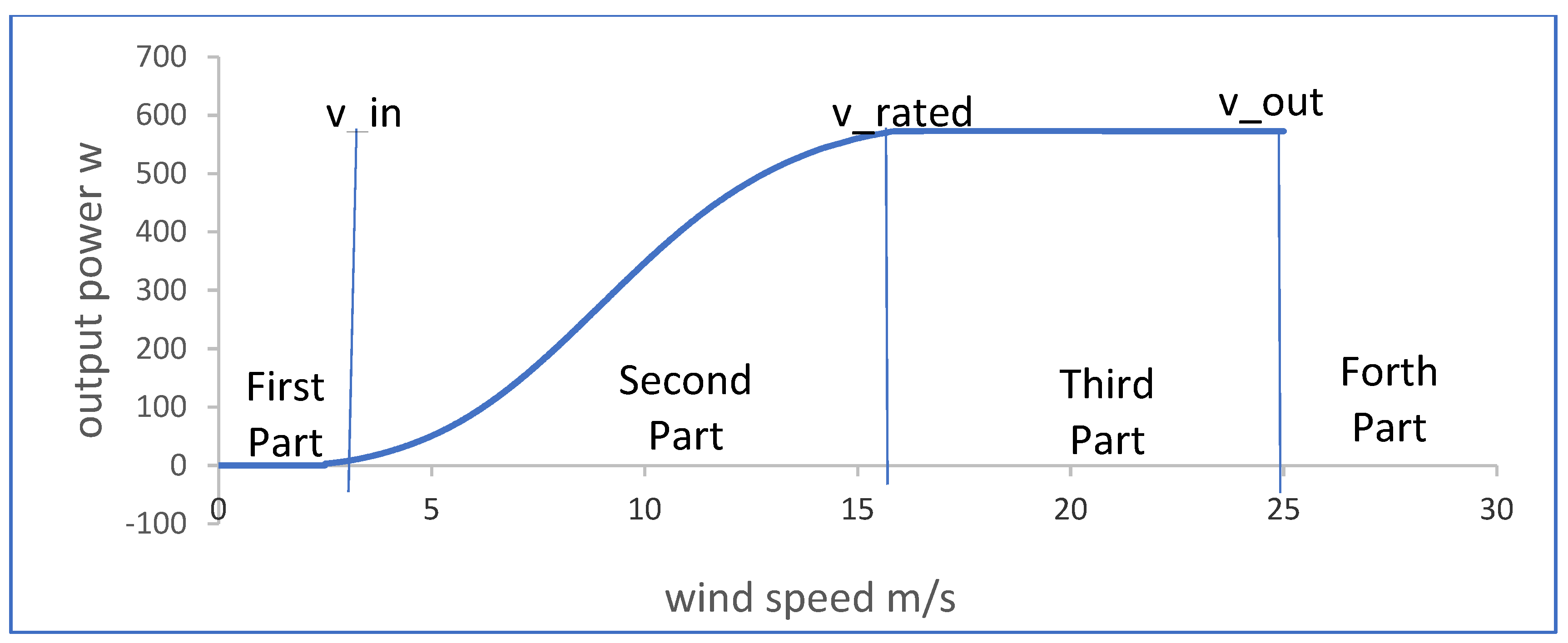
Figure 8 depicts the power curve that is produced in terms of wind speed.
From Figure 8, the power curve is divided into four major parts. The first part occurs at wind speed less than cut-in speed, which leads to zero output power. In the second part, the wind speed is between cut-in ( v i n ) and rated speed ( v r ), while the output power has nonlinear characteristics. The wind turbine output power has a constant value of rated output power for all models when the wind speed value is located between the rated and cut-out speed, as shown in the third part. To protect the wind turbine from damage, the wind turbine must be stopped when the wind speed becomes greater than the cut-out speed ( v o u t ) [30]. In the literature, various models have been used to describe this nonlinear relationship, such as the third-degree polynomial curve in ref. [21], as well as fitted polynomial function as in refs. [35,36]. The general form can be represented by:
p ( v ) = {        p r v r     v     v co p r     g ( v )     v ci     v     v r 0         o t h e r w i s e
where g(v) represents the relationship between the wind speed and the wind turbine output power that can be formed in several models as follows [29,30]:
g 1 ( v ) = ( v v 1 v r v 1 ) ,
g 2 ( v ) = ( v v 1 v r v 1 ) 2 ,
g 3 ( v ) =   v 2 v 1 2 v r 2 v 1 2 ,
g 4 ( v ) =   v 3 v 1 3 v r 3 v 1 3 ,
g 5 ( v ) =   ( v v r ) 3 ,
g 6 ( v ) = ( v v 1 v r v 1 ) 3 ,
g 7 ( v ) = ( a 1 v 2 + a 2 v + a 3 ) ,
g 8 ( v ) = ( a 1 v 3 + a 2 v 2 + a 3 v + a 4 ) ,
g 9 ( v ) = ( a 1 v 4 + a 2 v 3 + a 3 v 2 + a 4 v + a 5 ) ,
where a 1 , a 2 , a 3 , a 4 , and a 5   are polynominal coefficients calculated in MATLAB by the polyfit function. According to the previous comparison between analytical and heuristic methods for estimation of the Weibull distribution parameters, the proposed AO method provides the best fit for wind speed distribution for the two sites. Therefore, its output shape and scaling factors of the Weibull parameters are utilized, and then the detailed models (g1g9) are considered to find the best model for each site. In order to compare the performance of these nine models in estimating the energy from a wind turbine, the error ( ε ) between the actual energy density ( E a c t u a l ) and estimated energy ( E f i t t e d   ) is calculated by the following expression [21]:
E a c t u a l = 1 A i = 1 N f a c t u a l ( v i ) p m , i ( v i ) ,
E f i t t e d = 1 A i = 1 N f f i t t e d ( v i ) p m , i ( v i ) ,
ε = E f i t t e d E a c t u a l E a c t u a l 100 .
The error of energy density results for two sites is calculated where the distributions of energy density error for the nine models are shown in Figure 9 and Figure 10 for the Zafarana and Shark El-Ouinate sites, respectively. From Figure 9, at the Zafarana site, the second model (g2) provides the minimum error of energy density of 5.728%. After that, the fourth (g4) and seventh (g7) models come with an error of energy density of 6.005 and 6.167%, respectively. On the other side, all the models illustrate close errors where there is no great divergence in the results, as the worst model provides an error of energy density of 6.593%. From Figure 10, at the Shark El-Ouinate site, the eigth model (g8), the cubic form, provides the minimum error of energy density of 13.2%. After that, the ninth (g4) and seventh (g7) models come with an error of energy density of 13.6 and 16.6%, respectively.

6. Conclusions

This paper investigates different analytical and heuristic techniques for optimal parameter estimation of the Weibull distribution parameters to analyze the wind speed profile for the Zafarana and Shark El-Ouinate sites, Egypt. In this study, four analytical methods of MLM, MM, EM, and EPFM, and other heuristic methods of PSO and AO algorithms are introduced. Several fitness metrics are evaluated for comparative assessment between the competitive methods. The novel meta-heuristic AO algorithm shows the best performance in acquiring the highest value of R2, the least value of RMSE, and the least value of MAE for tuning Weibull PDF parameters. Additionally, the mean objective obtained by the AO algorithm is better than the others. Further, the AO algorithm is the most robust technique as it achieves the least standard deviation and standard error compared to the others. Furthermore, the AO algorithm demonstrates the greatest stability characteristics as its histogram of the obtained objectives is better than the PSO algorithm. Moreover, the AO algorithm presents the fastest convergence compared to the other since it provides its best solution through the first and second site parameters calculation, respectively. Furthermore, different models are analyzed to deduce the nonlinear relationship between the wind output power and the speed, where the error of wind energy density between actual and estimated is greatly minimized using the cubic model. A suggestion for future work is to obtain a rank for each method, where the mean wind speed and its standard deviation are estimated for a greater number of periods.

Author Contributions

Conceptualization, A.A.A.E.-E. and R.A.E.-S.; methodology, A.M.S.; software, A.S.S.; validation, R.A.E.-S., A.A.A.E.-E. and A.M.S.; formal analysis, A.S.S. and A.M.S.; investigation, A.S.S.; resources, A.A.A.E.-E.; data curation, R.A.E.-S.; writing—original draft preparation, A.S.S.; writing—review and editing, R.A.E.-S., A.M.S. and A.S.S.; visualization, A.A.A.E.-E.; supervision, A.A.A.E.-E.; project administration, R.A.E.-S.; funding acquisition, R.A.E.-S. All authors have read and agreed to the published version of the manuscript.

Funding

This research received no external funding.

Institutional Review Board Statement

Not applicable.

Informed Consent Statement

Not applicable.

Data Availability Statement

Not applicable.

Conflicts of Interest

The authors declare no conflict of interest.

Abbreviations

AOAquila optimizer
EMEmpirical method
EPFMEnergy pattern factor method
LSMLeast square method
MAEMean absolute error
MLMMaximum likelihood method
MMMoment method
MMOMModified method of moment
PDPower density method
PDFProbability density function
PSOParticle warm optimization
R2Determination coefficient
RMSERoot mean square error
WEEWind energy error
WEIMWind energy intensification method
WPDWind production deviation
RCorrelation coefficient
kShape factor
cScaling factor
f ( v ) Weibull probability distribution function
F ( v ) Weibull cumulative distribution function
nNumber of bins performed
v i Peed in time step i from time series data
σ Standard deviation of wind speed
y i Probability distribution of Weibull
x i Probability distribution of actual wind speed
y ¯ Probability of the mean wind speed
ρ Air density in (kg/m3)
STEStandard error
STDStandard deviation
a 1 , a 2 , a 3 , a 4 , and a 5 Polynomial coefficients
v i n Cut-in speed
v r Rated speed
v o u t Cut-out speed
E a c t u a l Actual energy density
E f i t t e d Estimated energy
p m ( v i ) Wind output power of the model (m) at wind speed ( v i )
A Swept area
f a c t u a l ( v i ) Frequency of wind speed from histogram at speed ( v i )
f f i t t e d ( v i ) Weibull distribution of wind speed ( v i )
TMaximum number of iterations

References

  1. Abaza, A.; Fawzy, A.; El-Sehiemy, R.A.; Alghamdi, A.S.; Kamel, S. Sensitive reactive power dispatch solution accomplished with renewable energy allocation using an enhanced coyote optimization algorithm. Ain Shams Eng. J. 2020, 12, 1723–1739. [Google Scholar] [CrossRef]
  2. Elsakaan, A.A.; El-Sehiemy, R.A.; Kaddah, S.S.; Elsaid, M.I. Optimal economic–emission power scheduling of RERs in MGs with uncertainty. IET Gener. Transm. Distrib. 2020, 14, 37–52. [Google Scholar] [CrossRef]
  3. Quan, H.; Khosravi, A.; Yang, D. A Survey of Computational Intelligence Techniques for Wind Power Uncertainty Quantification in Smart Grids. IEEE Trans. Neural Netw. Learn. Syst. 2019, 31, 4582–4599. [Google Scholar] [CrossRef] [PubMed]
  4. Shaheen, A.M.; Elattar, E.E.; El, R.A.; Senior, S.; Elsayed, A.M. An Improved Sunflower Optimization Algorithm Based-Monte Carlo Simulation for Efficiency Improvement of Radial Distribution Systems Considering Wind Power Uncertainty. IEEE Access 2020, 9, 2332–2344. [Google Scholar] [CrossRef]
  5. Shaheen, A.M.; Ginidi, A.R.; El-Sehiemy, R.A.; Elattar, E.E. Optimal economic power and heat dispatch in Cogeneration Systems including wind power. Energy 2021, 225, 120263. [Google Scholar] [CrossRef]
  6. Abdul-hamied, D.T.; Shaheen, A.M.; Salem, W.A.; Gabr, W.I.; El-sehiemy, R.A. Equilibrium optimizer based multi dimensions operation of hybrid AC/DC grids. Alex. Eng. J. 2020, 59, 4787–4803. [Google Scholar] [CrossRef]
  7. Abou El-Ela, A.A.; El-Sehiemy, R.A.; Shaheen, A.M.; Diab, A.E.G. Design of cascaded controller based on coyote optimizer for load frequency control in multi-area power systems with renewable sources. Control Eng. Pract. 2022, 121, 105058. [Google Scholar] [CrossRef]
  8. Alrashidi, M.; Pipattanasomporn, M.; Rahman, S. Metaheuristic Optimization Algorithms to Estimate Statistical Distribution Parameters for Characterizing Wind Speeds. Renew. Energy 2020, 149, 664–681. [Google Scholar] [CrossRef]
  9. Yan, J.; Liu, Y.; Han, S.; Wang, Y.; Feng, S. Reviews on uncertainty analysis of wind power forecasting. Renew. Sustain. Energy Rev. 2015, 52, 1322–1330. [Google Scholar] [CrossRef]
  10. Rocha, P.A.C.; de Sousa, R.C.; de Andrade, C.F.; da Silva, M.E.V. Comparison of seven numerical methods for determining Weibull parameters for wind energy generation in the northeast region of Brazil. Appl. Energy 2012, 89, 395–400. [Google Scholar] [CrossRef]
  11. Carneiro, T.C.; Melo, P.; Carvalho, P.C.M.; Braga, A.P.D.S. Particle Swarm Optimization method for estimation of Weibull parameters: A case study for the Brazilian northeast region. Renew. Energy 2016, 86, 751–759. [Google Scholar] [CrossRef]
  12. Pobočíková, I.; Michalková, M. Application of four probability distributions for wind speed modeling. Procedia Eng. 2017, 192, 713–718. [Google Scholar] [CrossRef]
  13. Saleh, H.; Aly, A.A.E.; Abdel-hady, S. Assessment of different methods used to estimate Weibull distribution parameters for wind speed in Zafarana wind farm, Suez Gulf, Egypt. Energy 2012, 44, 710–719. [Google Scholar] [CrossRef]
  14. Akdağ, S.A.; Dinler, A. A new method to estimate Weibull parameters for wind energy applications. Energy Convers. Manag. 2009, 50, 1761–1766. [Google Scholar] [CrossRef]
  15. Shoaib, M.; Siddiqui, I.; Khan, S.; Alhems, L.M. Assessment of wind energy potential using wind energy conversion system. J. Clean. Prod. 2019, 216, 346–360. [Google Scholar] [CrossRef]
  16. Shaban, A.H.; Resen, A.K.; Bassil, N. Weibull parameters evaluation by different methods for windmills farms. Energy Rep. 2020, 6, 188–199. [Google Scholar] [CrossRef]
  17. Rahman, S.M.; Chattopadhyay, H. A new approach to estimate the Weibull parameters for wind energy assessment: Case studies with four cities from the Northeast and East India. Int. Trans. Electr. Energy Syst. 2020, 30, e12574. [Google Scholar] [CrossRef]
  18. Celik, A.N. A statistical analysis of wind power density based on the Weibull and Rayleigh models at the southern region of Turkey. Renew. Energy 2003, 29, 593–604. [Google Scholar] [CrossRef]
  19. Chaurasiya, P.K.; Ahmed, S.; Warudkar, V. Study of different parameters estimation methods of Weibull distribution to determine wind power density using ground based Doppler SODAR instrument. Alex. Eng. J. 2018, 57, 2299–2311. [Google Scholar] [CrossRef]
  20. Kumar, K.S.P.; Gaddada, S. Statistical scrutiny of Weibull parameters for wind energy potential appraisal in the area of northern Ethiopia. Renew. Wind. Water Sol. 2015, 2, 14. [Google Scholar] [CrossRef] [Green Version]
  21. Usta, I. An innovative estimation method regarding Weibull parameters for wind energy applications. Energy 2016, 106, 301–314. [Google Scholar] [CrossRef]
  22. Sumair, M.; Aized, T.; Asad, S.; Gardezi, R.; Ubaid, S.; Muhammad, S.; Rehman, S. A newly proposed method for Weibull parameters estimation and assessment of wind potential in Southern Punjab. Energy Rep. 2020, 6, 1250–1261. [Google Scholar] [CrossRef]
  23. Sumair, M.; Aized, T.; Asad, S.; Gardezi, R.; Ubaid, S.; Muhammad, S.; Rehman, S. A novel method developed to estimate Weibull parameters. Energy Rep. 2020, 6, 1715–1733. [Google Scholar] [CrossRef]
  24. Collins, R.A.; Green, R.D. Statistical Methods for Bankruptcy Forecasting. J. Econ. Bus. 1982, 34, 349–354. [Google Scholar] [CrossRef]
  25. Saeed, M.A.; Ahmed, Z.; Yang, J.; Zhang, W. An optimal approach of wind power assessment using Chebyshev metric for determining the Weibull distribution parameters. Sustain. Energy Technol. Assess. 2020, 37, 100612. [Google Scholar] [CrossRef]
  26. Wang, J.; Hu, J.; Ma, K. Wind speed probability distribution estimation and wind energy assessment. Renew. Sustain. Energy Rev. 2016, 60, 881–899. [Google Scholar] [CrossRef]
  27. Freitas, C.; Lindemberg, D.A.; Marcus, S.; Macedo, V.S.; Costa, P.A.; Gomes, F.F. Four heuristic optimization algorithms applied to wind energy: Determination of Weibull curve parameters for three Brazilian sites. Int. J. Energy Environ. Eng. 2019, 10, 1–12. [Google Scholar] [CrossRef]
  28. Abbasi, B.; Hamid, A.; Jahromi, E.; Arkat, J.; Hosseinkouchack, M. Estimating the parameters of Weibull distribution using simulated annealing algorithm. Appl. Math. Comput. 2006, 183, 85–93. [Google Scholar] [CrossRef]
  29. Carrillo, C.; Montaño, A.O.; Cidrás, J.; Díaz-Dorado, E. Review of power curve modelling for wind turbines. Renew. Sustain. Energy Rev. 2013, 21, 572–581. [Google Scholar] [CrossRef]
  30. Akdağ, S.A.; Güler, Ö. A Comparison of Wind Turbine Power Curve Models. Energy Sources Part A Recover. Util. Environ. Eff. 2011, 33, 2257–2263. [Google Scholar] [CrossRef]
  31. Chang, T.; Wu, Y.; Hsu, H. Assessment of wind characteristics and wind turbine characteristics in Taiwan. Renew. Energy 2003, 28, 851–871. [Google Scholar] [CrossRef]
  32. Okafor, E.G.; Ezugwu, O.E.; Jemitola, P.O.; Sun, Y.; Lu, Z. Weibull Parameter Estimation Using Particle Swarm Optimization Algorithm. Int. J. Eng. Technol. 2018, 7, 7–10. [Google Scholar] [CrossRef]
  33. Abualigah, L.; Yousri, D.; Abd Elaziz, M.; Ewees, A.A.; Al-Qaness, M.A.; Gandomi, A.H. Aquila Optimizer: A novel meta-heuristic optimization Algorithm. Comput. Ind. Eng. 2021, 157, 107250. [Google Scholar] [CrossRef]
  34. Renewables.ninja. Available online: http://www.renewables.ninja (accessed on 23 January 2022).
  35. Hemmati, R.; Hooshmand, R.A.; Khodabakhshian, A.A. Reliability constrained generation expansion planning with consideration of wind farms uncertainties in deregulated electricity market. Energy Convers. Manag. 2013, 76, 517–526. [Google Scholar] [CrossRef]
  36. Yang, W.; Zhao, X.; Zhang, A.; He, C.; Qi, C. Coordinated Planning of Grid-connected Wind Farms and Grid Expansion Considering Uncertainty of Wind Generation. In Proceedings of the 2020 Asia Energy and Electrical Engineering Symposium (AEEES), Chengdu, China, 29–31 May 2020; pp. 782–787. [Google Scholar]
Figure 1. Flowchart of the AO for optimal estimation of Weibull parameters.
Wind 02 00033 g001
Figure 2. Weibull distributions: Zafarana site.
Wind 02 00033 g002
Figure 3. Weibull distributions: Shark El-Ouinate site.
Wind 02 00033 g003
Figure 4. Bar chart of each run for Zafarana site.
Wind 02 00033 g004
Figure 5. Bar chart of each run for Shark El-Ouinate site.
Wind 02 00033 g005
Figure 6. Convergence curves of the compared algorithms for Zafarana site.
Wind 02 00033 g006
Figure 7. Convergence curves of the compared algorithms for Shark El-Ouinate site.
Wind 02 00033 g007
Figure 8. Typical wind turbine power curve.
Wind 02 00033 g008
Figure 9. Energy density error of the nine models for Zafarana site.
Wind 02 00033 g009
Figure 10. Energy density error of the nine models for Shark El-Ouinate site.
Wind 02 00033 g010
Table 1. Wind turbine characteristics.
SiteZafaranaShark El-Ouinat
Wind Turbine TypeNordex N43Nordex-N100
Rated power (Pr) (kw)6002500
Hub height (m)55100
Cut-in wind speed (m/s)2.53
Cut-off wind speed (m/s)2525
Rated wind speed (m/s)1512.5
Table 2. Statistics analysis of wind speed data.
ParametersZafarana (m/s)Shark El-Ouinat (m/s)
Mean7.14686.4966
Maximum15.89713.508
Minimum1.80.077
Standard deviation1.86662.5139
Variance3.48446.3198
Table 3. Statistical analysis: Zafarana site, 2019 [34].
MethodCKR2RMSEMAEWPD
EPF7.9385543.5377460.9587870.0142170.01132−0.79318
MM7.8225094.5893750.9725450.0116040.007059−0.8114
EMP7.8523974.2972480.988490.0075130.005485−0.80762
MLM7.8527994.1987480.9906960.0067550.005216−0.80692
PSO7.84287364.16825880.99107710.00661510.0051341−0.80742
AO7.83818184.11382220.99135700.00651050.0051603−0.80716
Table 4. Statistical analysis: Shark El-Ouinate site, 2019.
MethodCKR2RMSEMAEWPD
MM7.2951152.8075040.8924560.0147190.011650−0.71425
MLM7.2669212.7905550.8883870.0149960.011920−0.71669
EMP7.2954512.8041190.8929580.0146850.011638−0.71404
PDF7.2982812.7753320.8968930.0144130.011540−0.71221
PSO7.7949832.6856060.9412940.0108750.009005−0.64316
AO7.7154742.6629660.9425920.0107550.008761−0.65233
Table 5. Statistical results of convergence characteristics: Zafarana site.
STDSTEBestWorstMean
PSO0.0053072610.000750560.0006563960.0227945030.006801911
AO1.7788 × 10−52.51561 × 10−60.0006358090.0007171860.000649055
Table 6. Statistical results of convergence characteristics: Shark El-Ouinate site.
STDSTEBestWorstMean
PSO0.0042780.0006050.0017740.0205850.006692
AO1.69 × 10−52.4 × 10−60.0017350.0018270.001749
Publisher’s Note: MDPI stays neutral with regard to jurisdictional claims in published maps and institutional affiliations.

