
Machine Learning Methods for Super-Kamiokande Solar Neutrino Classification †


Department of Physics and Astronomy, University of California at Irvine, Irvine, CA 92697, USA
†
Presented at the 23rd International Workshop on Neutrinos from Accelerators, Salt Lake City, UT, USA, 30–31 July 2022.
Phys. Sci. Forum 2023, 8(1), 42; https://doi.org/10.3390/psf2023008042
Published: 18 August 2023
Abstract
:Super-Kamiokande (SK) has observed solar neutrino recoil electrons at kinetic energies as low as 3.49 MeV to study neutrino flavor conversion within the sun. At SK-observable energies, these conversions are dominated by the Mikheyev–Smirnov–Wolfenstein (MSW) effect. An “upturn” in the electron neutrino survival probability in which vacuum neutrino oscillations become dominant is predicted to occur at lower energies, but radioactive background increases exponentially with decreasing energy. New machine learning approaches, including convolutional neural networks trained on photomultiplier tube data and boosted decision trees trained on reconstructed variables, provide substantial background reduction in the 2.49–3.49 MeV energy region such that the statistical extraction of solar neutrino interactions becomes feasible.
1. Introduction
1.1. The Super-Kamiokande Experiment
Super-Kamiokande (SK) is a 50 kton cylindrical water Cherenkov detector 1 km under Mt. Ikeno in Gifu, Japan [1]. The inner detector contains 11,129 twenty-inch PMTs that detect Cherenkov light emitted by particles traveling through the detector volume with energies above the Cherenkov threshold. The DAQ records events through two independent triggering systems. The software trigger saves an event when the number of hits in any 200 ns window surpasses a threshold, which is adjusted over time as needed according to the current dark noise rate. The wideband intelligent trigger (WIT) implemented in July 2015 runs parallel to the software trigger and instead performs online vertex reconstruction in order to preserve lower-energy events with near 100% triggering efficiency at 2.49 MeV electron kinetic energy [2]. In September 2018, SK completed SK-IV, the longest phase of the experiment, lasting 10 years. This phase is ideal for solar neutrino analyses due to upgraded front-end electronics as well as lower noise and radioactive background levels compared to previous phases.
1.2. Solar Neutrinos and the MSW Effect
Solar neutrinos can be observed in SK though elastic scattering on electrons because the maximum weak scattering angle of 15° relative to the solar direction is smaller than the >30° direction resolution at low energies [3]. With the completion of SK-IV, solar neutrino events have been observed with enough statistics to conduct detailed measurements, such as measurements of the solar neutrino flux, energy spectrum, and flavor conversion within the sun and earth [4]. At SK-observable energies of recoil electrons, the majority of observed solar neutrinos originate from decay in the solar fusion process, and their flavor conversion within the sun is dominated by the Mikheyev–Smirnov–Wolfenstein (MSW) effect [5]. Through the MSW effect, few-MeV-scale electron neutrinos produced in the core of the sun pass through a resonant density region and undergo an adiabatic conversion to the second mass neutrino eigenstate. This conversion becomes less likely to occur at lower energies such that the standard vacuum neutrino oscillations begin to dominate. This transition from MSW-dominated conversions to vacuum-dominated conversions leads to an “upturn” in the electron neutrino survival probability . The MSW effect and the implied upturn is a robust prediction of electro-weak physics, but the prevalence of radioactive decays producing electrons in this energy region has made it difficult for neutrino detectors to observe this phenomenon.
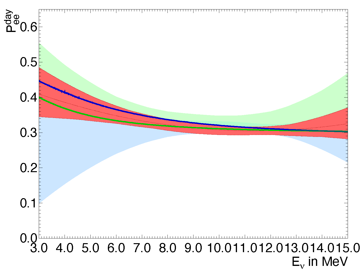
At the Neutrino conference in June 2022, Super-Kamiokande presented the latest fits to as a function of neutrino energy using the complete SK-IV dataset in combination with KAMLAND and SNO data (Figure 1). Statistical uncertainties remain large in the upturn region, but quadratic (exponential) fits to the recoil electron energy spectrum now disfavor an energy-independent by () [6].
1.3. Sources of Background
The largest source of background for low-energy analyses in SK is the Bi β decay that occurs during the decay process of radon (Rn) gas naturally found in the mine [7]. Carefully controlled convective currents within the inner detector make it possible to gather the Rn near the walls and in the bottom half of the detector to preserve a fiducial volume with a relatively low Rn concentration. The next-largest source is
Ti β rays originating from the PMT glass. These events are located exclusively near the walls but occasionally reconstruct within the fiducial volume in coincidence with dark noise hits. The WIT system triggers from events per day from these two sources of radioactive background. SK experiences a cosmic ray muon rate of 2 Hz as well. Muon-induced hadronic showers create a source of background for low-energy analyses through resulting radioactive nuclei and following decays [8].
1.4. Multiple Scattering Goodness
In addition to the event energy calculated from the light yield, multiple scattering goodness (MSG) is extensively used in SK solar analyses [4]. Since multiple Coulomb scattering increases with decreasing energy, low-energy events generate additional Cherenkov cones that do not align well with that of the initial vertex. MSG ranging from 0 to 1 quantifies the degree of alignment between the most likely direction fits of an event, with values closer to 1 indicating better alignment and therefore less scattering.
1.5. Outline
Traditional cut-based event selection methods currently do not provide sufficient background rejection to observe a solar neutrino signal in the low-energy, background-dominated region. These proceedings present the results of applying new machine learning methods to low-energy solar neutrino event selection with the purpose of improving background rejection and lowering the energy threshold of the SK solar analysis. Section 2 discusses the methods for generating the datasets used for training and testing, introduces the machine learning-based classifiers, and explains the solar angle fitting procedures for the final event selection. Section 3 presents the results of testing the various classifiers on an evaluation dataset, followed by the results of applying a boosted decision tree to SK-IV WIT data. Section 4 summarizes the findings and discusses future work.
2. Methods
2.1. Dataset Generation
Monte Carlo (MC) signal datasets were generated using software for the generation of solar neutrino interaction vertices and to simulate the SK detector. For the training dataset, the existing vertex generation was modified to randomize the vectors of the direction of electron recoil in order to obscure the solar direction from the classifiers since the solar direction relative to the detector is not uniformly distributed over time and the classifiers may learn to recognize this trend. This modification makes it possible to evaluate the classifiers’ performance through the solar angle distributions of their data selections. The MC events without dark noise were then inserted into dummy trigger windows containing real, untriggered raw data, and the resulting collections of hits were then fed to the WIT triggering algorithm. The MC events were then extracted by identifying triggered events with reconstructed vertex times within 300 ns of the true MC vertex times. Due to the limited amount of SK-IV raw data available for the purpose of noise overlay, the training/validation dataset was generated such that each MC event was inserted in a unique trigger window to eliminate possible training bias due to repeated noise patterns, while trigger windows used for the evaluation dataset were reused a maximum of four times for different MC events. The former dataset was randomly split into 1.14 million training and 0.14 million validation events, and the isolated evaluation dataset consisted of 1.46 million events. These datasets consisted of equal parts signal and background to eliminate event class bias. Since SK-IV WIT data were subjected to first reduction cuts, which reduced the event rate to events per day due to data storage limitations, the same cuts were applied to the triggered MC events. Real WIT data drawn from various points in the SK-IV WIT data-taking period was used for the background sample in the training and evaluation datasets because background events outnumber signal events by approximately seven orders of magnitude.
2.2. Boosted Decision Tree
A boosted decision tree (BDT) [9] was trained on the reconstructed variables used in the traditional SK solar analysis [4]. These variables included the event energy, MSG, direction vector, distance from the vertex to the wall, position of the wall intersecting with the reverse direction vector, and the distance between the vertex and this wall position. Goodness-of-fit metrics based on small clusters of PMT hits, vertex fit timing residuals , the Cherenkov cone symmetry , and their combination were also included. In addition to existing variables, the distance to the tight fiducial volume boundary as well as the value of a th, th)-degree 2D polynomial fit of the spatial background distribution in were added as inputs to improve the BDT’s background reduction. The variables with the most impact on the BDT’s decision were the distance to the wall and .
2.3. ResNet
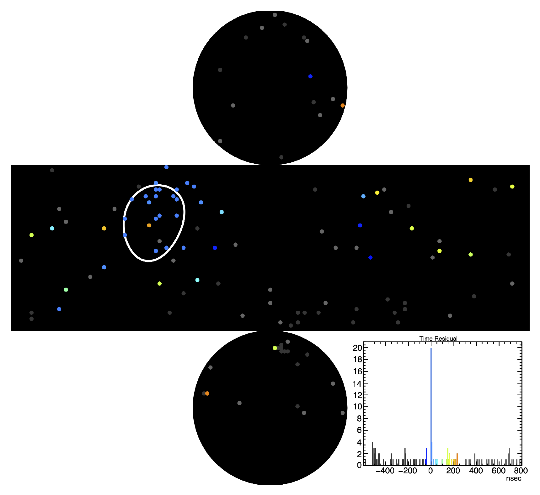
A modified version of the ResNet18 convolutional neural network [10] developed by the water Cherenkov machine learning group (WatChMaL) [11] was trained with 147 × 149 2D event display images of hit PMTs (Figure 2). Each pixel contained two channels with the PMT hit charge and hit time relative to the reconstructed vertex time.
2.4. Solfit
Following each networks’ data selection process, SK’s existing methods for extracting solar neutrino events from solar angle distributions were used [4]. A background shape was first generated using the “scramble” method, in which a solar angle histogram was filled with for all possible pairs of event directions and solar directions in the data sample. This method generated a background shape that incorporated effects from biases, such as the detector’s shape or event locations, that were independent of solar direction. A signal shape was then generated using a polynomial fit to the solar angle distribution of separately generated MC signals, now with solar direction preserved. The “solfit” extended unbinned maximum likelihood fitter then calculated the number of solar neutrino interactions in the sample using solar angle probability distribution functions for the signal and background.
3. Results
3.1. Network Evaluation
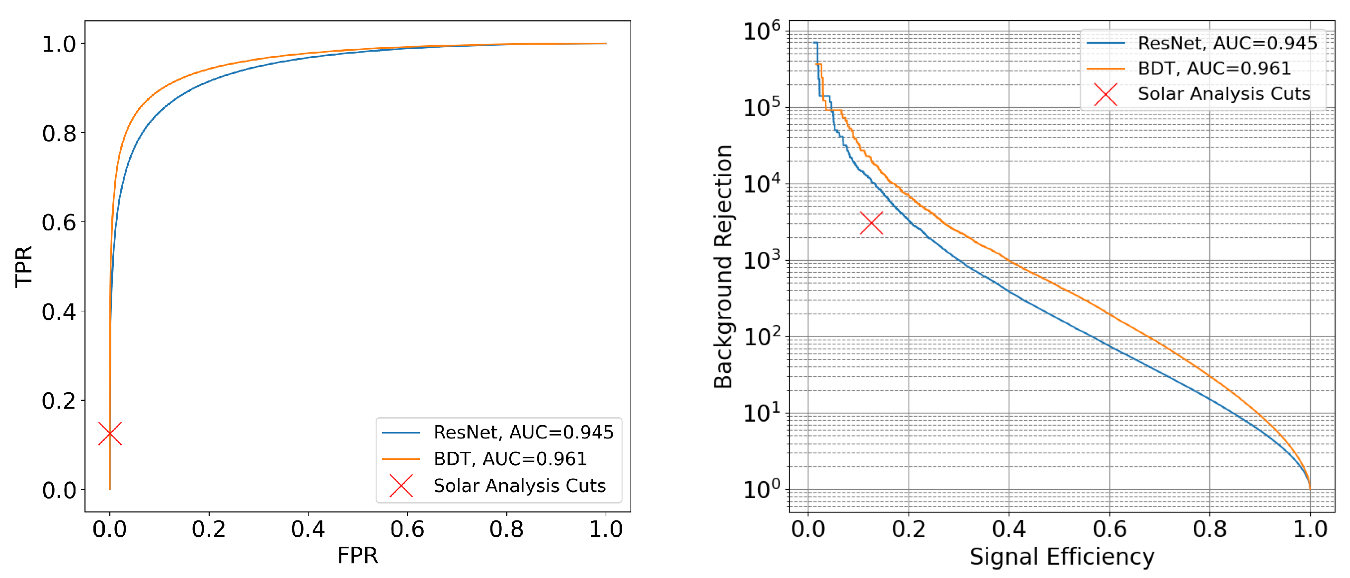
A receiver operating characteristic (ROC) curve that plots the background reduction defined as the inverse of the background efficiency as a function of signal efficiency can be used to evaluate the classification performance of the available methods on the evaluation dataset. The ROC curve (Figure 3) shows that both methods can provide increased sensitivities with the BDT giving 6× the background reduction with the same signal efficiency as the traditional cuts in the 2.49–3.49 MeV electron kinetic energy region of interest.
3.2. BDT Implementation
The BDT, ResNet, and traditional SK solar analysis cuts were applied to all available SK-IV WIT events with 2.49–3.49 MeV kinetic energy. At the time of the NuFact 2022 conference, the BDT’s implementation was complete, but ResNet’s implementation was ongoing due to its considerable computational requirements.
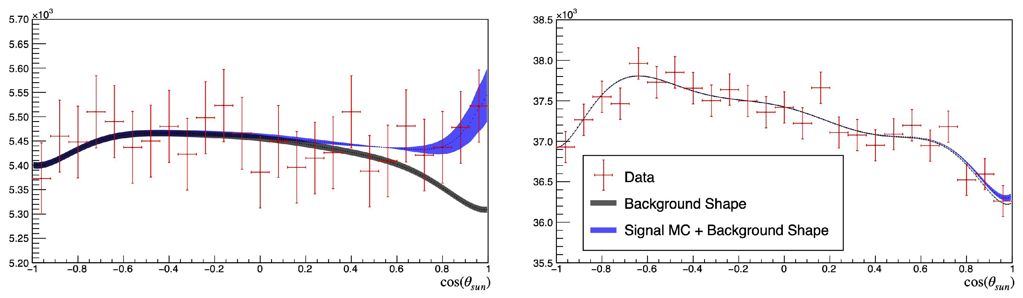
The solar angle distributions, signal and background shapes (Figure 4), and corresponding number of fit signal events with statistical uncertainties (Table 1) for the BDT and traditional cuts are shown. The cut for the BDT’s output was chosen to match the expected signal efficiency of the traditional cuts according to the ROC curve generated with the evaluation dataset described in Section 2.1.
These total event rates show that the BDT provides the expected increase in background reduction on this full dataset, as implied by the ROC curves. The solfit results also suggest a greater number of signal events for the BDT selection than for the traditional cuts.
The results of the individual sub-bins indicate that most of the BDT’s observed signal events are from the higher-energy and higher MSG sub-bins. This trend is likely due to the fact that the energy and MSG variables are inputs for the BDT, while the traditional cuts are constant over this energy range. Since the background rate increases with decreasing energy, the cut selection reflects this trend, while the BDT selects fewer events.
4. Discussion
The results of the BDT selection and number of signal events determined by solfit suggest a hint of a solar neutrino signal in this very-low-energy region. The errors reported here are statistical uncertainty only, and a systematic error analysis must be conducted. We expect the systematic error to be larger than the statistical error because the fit number of signal events may vary widely depending on the cut value used for the BDT output. Although the results imply that a signal can be observed with the current signal-to-noise ratio, the solfit maximum likelihood function may still be unstable when near the necessary threshold for an observable signal. Other possible sources of systematic error include the background shape calculation method, MC generation method, and BDT training procedure, such as the choice of variables. We plan to compute the livetime of the WIT data sample and compare the observed signal event rate to that of the theoretical rate with and without MSW oscillations as a method of validation and as further indication of whether a signal can be observed using a selection method with slightly higher sensitivity.
Additional approaches we plan to investigate include a hybrid BDT/CNN approach that takes both reconstructed variables and event display images as input, as well as other types of networks, such as graph neural networks or networks trained on point clouds that respect the cylindrical geometry of the detector.
Funding
This research was funded by the National Science Foundation grant number PHY-2013073.
Institutional Review Board Statement
Not applicable.
Informed Consent Statement
Not applicable.
Data Availability Statement
The data analyzed in this article was collected by the Super-Kamiokande collaboration and is not publically available. The code is available upon request from the corresponding author.
Conflicts of Interest
The authors declare no conflict of interest.
References
- Fukuda, S.; Fukuda, Y.; Hayakawa, T.; Ichihara, E.; Ishitsuka, M.; Itow, Y.; Kajita, T.; Kameda, J.; Kaneyuki, K.; Kasuga, S.; et al. The Super-Kamiokande detector. Nucl. Instr. and Meth. A 2003, 501, 418–462. [Google Scholar] [CrossRef]
- Elnimr, M.; Super-Kamiokande Collaboration. Low Energy 8B Solar Neutrinos with the Wideband Intelligent Trigger at Super-Kamiokande. J. Phys. Conf. Ser. 2017, 888, 012189. [Google Scholar] [CrossRef]
- Abe, K.; Super-Kamiokande Collaboration. Solar neutrino measurements in Super-Kamiokande-III. Phys. Rev. D 2011, 83, 052010. [Google Scholar] [CrossRef]
- Abe, K.; Haga, Y.; Hayato, Y.; Ikeda, M.; Iyogi, K.; Kameda, J.; Kishimoto, Y.; Marti, L.; Miura, M.; Moriyama, S.; et al. Solar neutrino measurements in Super-Kamiokande-IV. Phys. Rev. D 2016, 94, 052010. [Google Scholar] [CrossRef]
- Mikheyev, S.P.; Smirnov, A.Y. Resonant amplification of ν oscillations in matter and solar-neutrino spectroscopy. Il Nuovo Cimento C 1986, 9, 17–26. [Google Scholar] [CrossRef]
- Koshio, Y. Overview of the solar neutrino observation. In Proceedings of the Neutrino 2022 Conference, Seoul, Republic of Korea, 2 June 2022. [Google Scholar]
- Nakano, Y.; Hokama, T.; Matsubara, M.; Miwa, M.; Nakahata, M.; Nakamura, T.; Sekiya, H.; Takeuchi, Y.; Tasaka, S.; Wendell, R.A.; et al. Measurement of the radon concentration in purified water in the Super-Kamiokande IV detector. Nucl. Instr. Meth. A 2003, 977, 164297. [Google Scholar] [CrossRef]
- Zhang, Y.; Abe, K.; Haga, Y.; Hayato, Y.; Ikeda, M.; Iyogi, K.; Kameda, J.; Kishimoto, Y.; Miura, M.; Moriyama, S.; et al. First measurement of radioactive isotope production through cosmic-ray muon spallation in Super-Kamiokande IV. Phys. Rev. D 2016, 93, 012004. [Google Scholar] [CrossRef]
- Roe, B.P.; Yang, H.J.; Zhu, J.; Liu, Y.; Stancu, I.; McGregor, G. Boosted decision trees as an alternative to artificial neural networks for particle identification. Nucl. Instr. Meth. A 2005, 543, 577–584. [Google Scholar] [CrossRef]
- He, K.; Zhang, X.; Ren, S.; Sun, J. Deep Residual Learning for Image Recognition. In Proceedings of the 2016 IEEE Conference on Computer Vision and Pattern Recognition, Las Vegas, NV, USA, 27–30 June 2016; pp. 770–778. [Google Scholar]
- Prouse, N. Machine Learning Techniques for Water Cherenkov Event Reconstruction. In Proceedings of the CAP Congress, Virtual, 7 June 2021. [Google Scholar]
Figure 1.
Predicted vs. neutrino energy based on fits to electron energy spectrum of daytime events. The best quadratic fit for all solar experiments (green line), solar + KAMLAND (blue line), and region for SK (green band), SNO (blue band), and SK + SNO (red band) are shown.
Figure 1.
Predicted vs. neutrino energy based on fits to electron energy spectrum of daytime events. The best quadratic fit for all solar experiments (green line), solar + KAMLAND (blue line), and region for SK (green band), SNO (blue band), and SK + SNO (red band) are shown.

Figure 2.
A typical low-energy data event display with PMT relative times. The reconstructed Cherenkov cone is shown in white.
Figure 2.
A typical low-energy data event display with PMT relative times. The reconstructed Cherenkov cone is shown in white.

Figure 3.
Standard true-positive rate (TPR) vs. false-positive rate (FPR) ROC curve (left) and background rejection (inverse of FPR) vs. MC signal efficiency (TPR) ROC curve (right) for considered classification methods. Legend shows area under curve (AUC) for the standard ROC curve.
Figure 3.
Standard true-positive rate (TPR) vs. false-positive rate (FPR) ROC curve (left) and background rejection (inverse of FPR) vs. MC signal efficiency (TPR) ROC curve (right) for considered classification methods. Legend shows area under curve (AUC) for the standard ROC curve.

Figure 4.
Solar angle distribution for data selection (red), background shape (black), and signal + background shape (blue), all with statistical error bands for the BDT selection (left) and the traditional cut selection (right).
Figure 4.
Solar angle distribution for data selection (red), background shape (black), and signal + background shape (blue), all with statistical error bands for the BDT selection (left) and the traditional cut selection (right).


Table 1.
Total selected events and fit number of signal events with statistical error in each energy and MSG sub-bin used in the SK solar analysis. A range covering multiple sub-bins indicates that all included sub-bins are fit simultaneously.
Table 1.
Total selected events and fit number of signal events with statistical error in each energy and MSG sub-bin used in the SK solar analysis. A range covering multiple sub-bins indicates that all included sub-bins are fit simultaneously.
| Ekin Bin Range | MSG Bin Range | Total Events | Signal Interactions | ||
|---|---|---|---|---|---|
| BDT | Cuts | BDT | Cuts | ||
| 2.49–2.99 MeV | 0–0.35 | 8,004 | 498,341 | ||
| 2.49–2.99 MeV | 0.35–0.45 | 12,760 | 223,243 | ||
| 2.49–2.99 MeV | 0.45–1 | 17,110 | 111,957 | ||
| 2.99–3.49 MeV | 0–0.35 | 26,814 | 51,708 | ||
| 2.99–3.49 MeV | 0.35–0.45 | 31,125 | 28,701 | ||
| 2.99–3.49 MeV | 0.45–1 | 48,463 | 17,686 | ||
| 2.49–2.99 MeV | 0–1 | 37,874 | 833,541 | ||
| 2.99–3.49 MeV | 0–1 | 98,402 | 98,095 | ||
| 2.49–3.49 MeV | 0–1 | 136,276 | 931,636 | ||
Disclaimer/Publisher’s Note: The statements, opinions and data contained in all publications are solely those of the individual author(s) and contributor(s) and not of MDPI and/or the editor(s). MDPI and/or the editor(s) disclaim responsibility for any injury to people or property resulting from any ideas, methods, instructions or products referred to in the content. |
© 2023 by the author. Licensee MDPI, Basel, Switzerland. This article is an open access article distributed under the terms and conditions of the Creative Commons Attribution (CC BY) license (https://creativecommons.org/licenses/by/4.0/).
Share and Cite
MDPI and ACS Style
Yankelevich, A. Machine Learning Methods for Super-Kamiokande Solar Neutrino Classification. Phys. Sci. Forum 2023, 8, 42. https://doi.org/10.3390/psf2023008042
AMA Style
Yankelevich A. Machine Learning Methods for Super-Kamiokande Solar Neutrino Classification. Physical Sciences Forum. 2023; 8(1):42. https://doi.org/10.3390/psf2023008042
Chicago/Turabian StyleYankelevich, Alejandro. 2023. "Machine Learning Methods for Super-Kamiokande Solar Neutrino Classification" Physical Sciences Forum 8, no. 1: 42. https://doi.org/10.3390/psf2023008042