
Geometric Variational Inference and Its Application to Bayesian Imaging †


Max Planck Institute for Astrophysics, Karl-Schwarzschild-Straße 1, 85748 Garching, Germany
†
Presented at the 41st International Workshop on Bayesian Inference and Maximum Entropy Methods in Science and Engineering, Paris, France, 18–22 July 2022.
Phys. Sci. Forum 2022, 5(1), 6; https://doi.org/10.3390/psf2022005006
Published: 2 November 2022
(This article belongs to the Proceedings of The 41st International Workshop on Bayesian Inference and Maximum Entropy Methods in Science and Engineering)
Abstract
:Modern day Bayesian imaging problems in astrophysics as well as other scientific areas often result in non-Gaussian and very high-dimensional posterior probability distributions as their formal solution. Efficiently accessing the information contained in such distributions remains a core challenge in modern statistics as, on the one hand, point estimates such as Maximum a Posteriori (MAP) estimates are insufficient due to the nonlinear structure of these problems, while on the other hand, posterior sampling methods such as Markov Chain Monte Carlo (MCMC) techniques may become computationally prohibitively expensive in such high-dimensional settings. To nevertheless enable (approximate) inference in these cases, geometric Variational Inference (geoVI) has recently been introduced as an accurate Variational Inference (VI) technique for nonlinear unimodal probability distributions. It utilizes the Fisher–Rao information metric (FIM) related to the posterior probability distribution and the Riemannian manifold associated with the FIM to construct a set of normal coordinates in which the posterior metric is approximately the Euclidean metric. Transforming the posterior distribution into these coordinates results in a distribution that takes a particularly simple form, which ultimately allows for an accurate approximation with a normal distribution. A computationally efficient approximation of the associated coordinate transformation has been provided by geoVI, which now enables its application to real-world astrophysical imaging problems in millions of dimensions.
1. Introduction
Bayesian astrophysical imaging is a large and growing task within the field of astrophysics. It has a rather unique setting in the context of generic imaging problems. While the information provided by the data of modern telescopes is vast and very rich in detail, it remains almost negligible compared to the richness and complexity of the cosmos. Accurate uncertainty quantification is therefore an absolute necessity, but facing the real-world sizes of problems is a challenge. Numerical approximations are a common approach to tackle this issue. Recently, the software package Numerical Information Field Theory (NIFTy [1]) has been developed and continuously improved to provide a framework for algorithmic realizations to solve real-world imaging tasks. The recent version of NIFTy (https://gitlab.mpcdf.mpg.de/ift/nifty, accessed on 31 October 2022) provides the geometric Variational Inference (geoVI [2]) algorithm as its standard approximation method to solve inference problems. In this work the geoVI algorithm, its performance in the context of imaging, and the general problem setup of Bayesian astrophysical imaging are discussed.
1.1. Probabilistic Reasoning
In general, reasoning under uncertainty requires application of the updating rule for probabilities provided via the product rule. For well-defined cases, the derivation and intuitive validity of Bayes theorem is straightforward, provided the complete set of rules of probabilistic logic. Specifically, updating one’s belief about a signal s in light of novel (observational) information d, given the likelihood of retrieving this information , yields an updating rule of the form
In the simplest case of (Bayesian) astrophysical imaging, the signal s describes an image, e.g., the monochromatic brightness distribution of flux observable within a field of view (FOV). In this case, s is a scalar function that assigns a brightness value to each location within the FOV. In generic astro imaging problems, the scalar image is likely to be exchanged for a more complicated object such as an all-sky image in spherical coordinates [3,4,5,6], a multi-chromatic (multi-frequency) image [7,8], a time-variable [9,10] or vector-valued function [11], a three-dimensional function describing the density distribution of objects in our local galactic [12,13,14] or cosmic [15,16,17,18,19,20,21,22] neighborhood, or even a combination of multiple functions that have to be inferred simultaneously [23].
In all cases s is a field, i.e., an object with infinitely many degrees of freedom (DOF). In this work, the numerical approximation of distributions over images shall be discussed. A necessary prerequisite is the existence of a consistent discretization in order to represent the image on a computer. This results in a high—but finite—dimensional approximation of the original infinite dimensional inference problem. For the sake of simplicity, in this work, the existence of a consistent discretization is assumed, henceforth, only the finite dimensional representation of s shall be considered. From now on, s describes a real-(or complex-)valued vector that contains discretized values of a random process, and the distribution is defined over a continuous finite-dimensional configuration space. For a detailed discussion regarding the discretization consistency of random processes considered in this work, please refer to [24]. In contrast, the observational information (or data) d is by definition always finite dimensional. Nevertheless, in the context of astrophysical imaging, it is usually also very high-dimensional, as the information gathered by modern day telescopes is vast and extremely rich in detail in almost all areas of the field.
Finally, our prior knowledge regarding the cosmos as well as the measurement processes involved has grown vast and detailed, which in general yields prior and likelihood distributions that are non-conjugate and often give rise to non-Gaussian and intractable joint distributions .
1.2. Posterior Approximation
In order to access the information encoded within the updated distribution (aka the posterior) , integration over must be feasible. Intractable distributions, however, do not allow for analytic integration; therefore, approximations are a necessity. Fast and accurate approximation of continuous probability distributions is a longstanding problem within probability theory, and the approaches to its solution are vast and range from point estimates over variational inference methods [25,26,27,28,29,30,31] to direct posterior sampling techniques, such as Markov Chain Monte Carlo [32,33,34,35,36] and nested sampling methods [37,38,39]. In the context of astrophysical imaging a set of desired properties for any approximation method arises:
- Accuracy: The approximation must be accurate even in the case of non-Gaussian and non-conjugate posterior distributions.
- Scalability: Scalability in both the number of data points and the number of DOFs of s are of utmost importance. In practice, only methods with a quasilinear scaling in both are fast enough to cope with the sizes of realistic problems in astrophysical imaging.
- Efficiency: Any method must allow for an efficient implementation that makes use of available computational resources as well as possible, as linear scaling alone does not necessarily yield a fast approximation algorithm, if the resources are not used efficiently.
In this work, the implications of the geoVI method as an approximation algorithm for generic imaging and high-dimensional continuous inference tasks is discussed. GeoVI builds upon a strong foundation of well known and successful VI methods such as the mean-field (MF) approach [25], Automatic Differentiation VI (ADVI) [28], Metric Gaussian VI (MGVI) [40], and VI with Normalizing Flows (NF) [27] and additionally shares considerable conceptual overlap with a recently introduced MCMC method named Riemannian manifold Hamilton Monte Carlo (RMHMC) [41]. It aims to fulfill all the above desired properties for astrophysical imaging and provides a tunable tradeoff between the accuracy and the overall runtime of the approximation.
2. Geometric Variational Inference
In general, VI aims to approximate the intractable posterior distribution P via a tractable one Q, where the approximation Q is chosen such that it minimizes the forward Kullback–Leibler (KL) divergence between P and Q
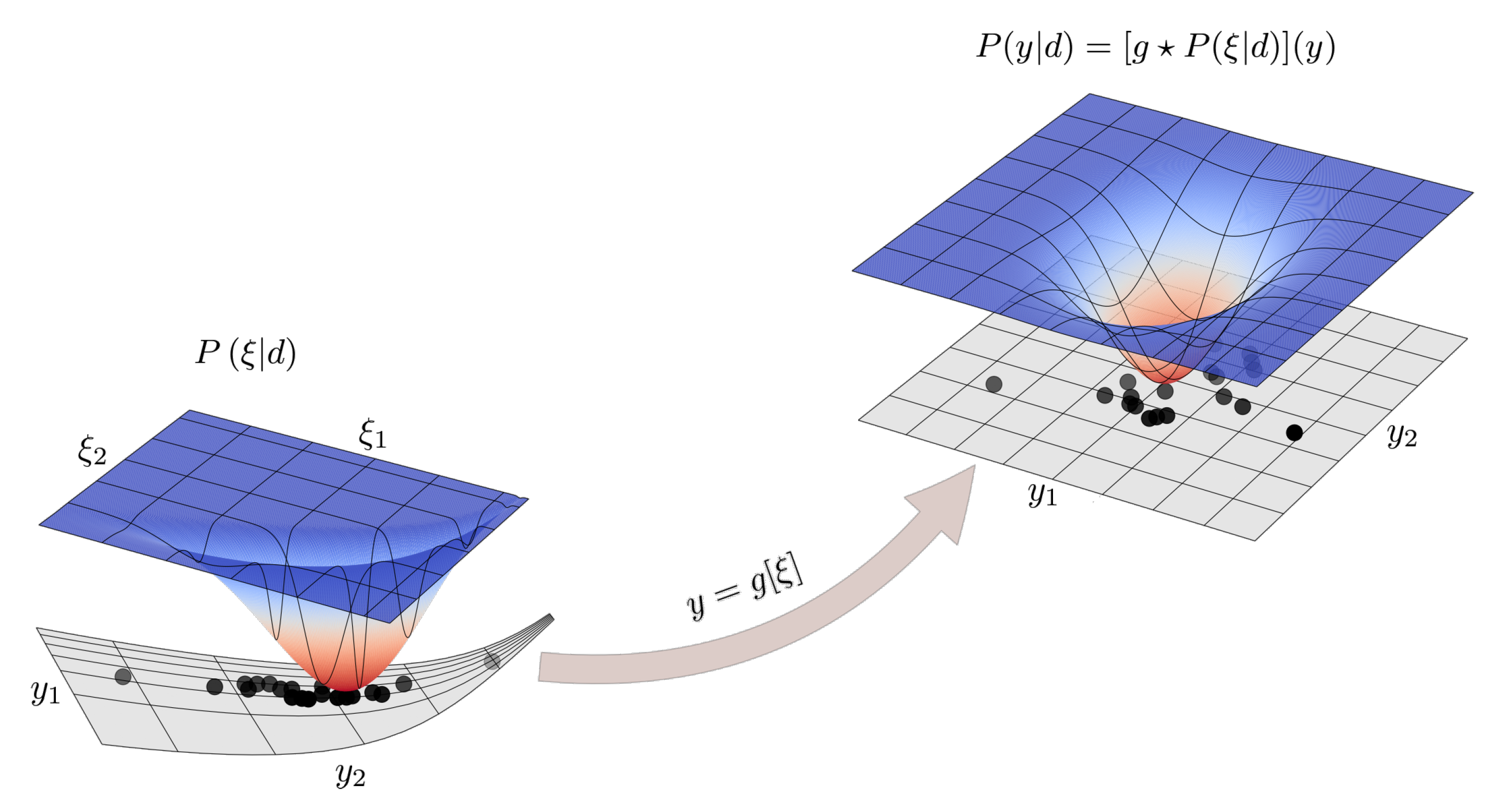
where stands for integration over the probability measure Q, and the right hand side is an approximation of the integral using a finite set of M random realizations generated from Q. The may be regarded as an information distance between probability distributions, and minimizing it yields minimal information difference between P and Q. As shown in [42], however, optimal approximation of information is achieved when minimizing the backward KL, i.e., , as this leads to a minimal loss of information when utilizing Q instead of P. In contrast, minimizing the forward KL yields, in some sense, a minimal gain of artificial information. Nevertheless, as can be seen by the Taylor expansion of the KL [2], the forward and backward KL are equivalent up to and including second order. Therefore, in the case where Q provides a close match for P, the result also becomes near optimal. In practice, typically a parametric family of distributions is defined, and the optimal parameter configuration is chosen via minimization of the with respect to m. The success of VI methods critically depends on the closeness of the parametric family to the true distribution. In geoVI, this closeness is achieved by deriving a coordinate transformation from the true posterior P, in which P approximately takes the form of a single standard normal distribution (in the case of multi-modality, it takes the form of multiple standard normal distributions), and approximating P in this coordinate system with a standard normal distribution Q (see Figure 1). The coordinate transformation is derived from the Fisher–Rao information metric (FIM) [43], associated with the distribution P.
Coordinate System
The full coordinate transformation consists of two consecutive steps. First, the posterior is reformulated in the standard coordinates of the prior distribution. The standard coordinate system is the one in which the prior takes the form of a standard normal distribution; therefore, a transformation may be set up such that
where ⋆ denotes the push-forward of a distribution represented in one coordinate system transformed into another one s via the transformation f. In the last term, we made the fact that is a standard normal distribution explicit.
Fisher–Rao Metric and Normal Coordinates
In the standard coordinate system of the prior, the posterior takes the form
This representation of the posterior is used to define the second transformation using the so-called metric of the posterior . This metric consists of the FIM of the likelihood , joined by the identity matrix serving as a distance measure from the curvature of the prior. is given in terms of the likelihood as
and the posterior metric is defined to be
where we additionally defined as the function that maps onto the coordinate system, where the FIM takes the form of the identity matrix. Here, † denotes the adjoint of a matrix. See [2] for a list of common likelihood classes, their metrics , and their associated transformations x.
The metric serves as the constructing point of the coordinate system utilized by geoVI. Specifically, a set of normal coordinates is constructed around a point m, where the metric becomes flat within a local neighborhood. The coordinates y and their associated transformation take the form
where denotes a function of being evaluated at m, and denotes the matrix square root of . See Figure 1 for a visualization of the effect of the coordinate transformation on probability densities.
Finally, the approximation Q is defined using the invertible transformation
The VI task reduces to optimizing the KL between P and with respect to the optimal expansion point m. In practice, this optimization problem is solved using a stochastic estimate of the KL and a set of samples generated from Q using the current best estimate of m.
3. A Simple Imaging Example
Two of the demands in Section 1.2, namely accuracy and efficiency have already been studied and discussed in [2] for the geoVI algorithm. For a posterior with a single sufficiently dominant mode the approximation becomes fairly accurate, in particular for distributions that deviate from a normal distribution in a monotonic fashion. It also allows for an efficient algorithmic realization due to the fact that both sample generation and model evaluation trivially parallelizes over multiple samples allowing for the usage of high-performance computing clusters. Only evaluating the KL requires an average over all samples (see Equation (2)) and therefore requires communication between nodes during runtime.
What remains to be demonstrated is the linear scalability of the algorithm. To do so, we set up a simple, yet realistic, two-dimensional imaging task and increased its resolution and number of measurements to study the scaling of the runtime of the algorithm as a function of resolution.
The mock imaging problem was given using a data model of the form
with N being the known noise covariance, and R denoting a linear measurement. For the simplest case, we chose R to be an evaluation operator that measures at multiple locations in space. For the displayed examples, R was set to measure ∼1% as many locations as there were numbers of pixels in the space on which s was discretized, which were randomly selected. Furthermore, N was set to be a diagonal matrix with the same noise standard deviation for all measurements. The log-signal s was assumed to a priori follow a statistically homogeneous and isotropic Gaussian random process, fully specified via its power spectrum . The functional form of was also assumed to be unknown a priori; therefore, it was to be inferred from the observations as well. A suitable prior for based on an integrated Wiener process on double-logarithmic scale, as well as the reformulation of the joint random process for s and as a generative process, was discussed in detail in [9]. Both quantities have to be inferred simultaneously, and their joint distribution was approximated using geoVI. Figure 2 displays the measurement setup, a mock example, and the reconstruction thereof. While the setup was simple and free from additional measurement effects such as point-spread functions, unknown or non-Gaussian noise statistics, and instrument calibration effects, it did cover the relevant challenges arising in imaging, such as a sparse and irregular measurement coverage (see top right panel of Figure 2) and missing prior information regarding relevant correlation scales. As can be seen, geoVI appears to be able to accurately solve such imaging problems. It not only recovered the distribution of s (and ) accurately but also the posterior distribution of . A detailed study of the overall reconstruction quality is beyond the scope of this work (see [2] for an in depth study). Nevertheless, qualitatively, we see that the posterior standard deviation map, shown in Figure 2, covered relevant aspects of the remaining posterior uncertainties. At the measurements, the uncertainty was small, and the information gained from these locations also informed their neighborhood. Multiple nearby measurements could also efficiently constrain a larger area together leading to a structured uncertainty map that depended on the measurement layout in a nontrivial fashion. Finally, the recovered posterior distribution of the prior spectra also qualitatively provided meaningful results. The uncertainty increased towards smaller scales (larger values of ) as the measurement setup overall provideed less information regarding these scales compared to larger scales.
Scaling Behavior
To verify the linear scaling, we repeated the same measurement setting while simultaneously increasing the number of pixels and number of measurements. The ratio of between pixels and measurements was held fixed. Note that increasing the number of pixels resulted in an even larger increase in the total number of DOF that had to be inferred, as also obtained additional DOF due to the fact that previously unresolved small scales became part of the inference problem enlarging the space on which was defined.
For simplicity, we switched the setup to a one-dimensional setting and defined s on a one-dimensional space. All other aspects (random measurements and the unknown prior correlation structure) of the imaging problem were retained, and the task remained to approximate the distribution of s and simultaneously. Figure 3 displays the runtime of the geoVI algorithm as a function of the number of DOF and number of data points. All size configurations were run 10 times, and the mean and standard deviation of the runtime are depicted. To avoid a bias towards specific configurations, all parameters of each run were regenerated randomly. This included: the mock spectrum , used to define the prior statistics from which a random realization of the signal s was drawn, the noise configuration n to define the data d, and the measurement locations of the response layout R. As can be seen in Figure 4, the variability of the spectral prior was large, leading to a variety of different mock setups. This variability translated into the overall runtime of geoVI. To ensure a valid comparison, we made use of the ground truth realization available to define a set of error measures between the ground truth, the data, and the reconstruction. Only in the case when all the error measures were within accepted ranges did we terminate the geoVI algorithm and claim convergence. The error measures are based on the root mean square values. Specifically,
where , , and stands for the total number of data points, DOFs, and pixels, respectively. and denote the posterior mean and variance recovered by geoVI for the respective quantities, denotes the standard coordinates of the prior distribution, and and are the mock (ground truth) realizations of the prior process used to generate the measurement data.
For each scaling run, convergence was defined once all three values were within the range . Together, this ensured that the algorithm’s output was comparable to the data within the measurement uncertainties, while simultaneously similar to the mock input signal, within the uncertainty estimate provided by geoVI itself. In addition, a maximal number of iteration steps was set, as for some realizations the method did not reach convergence in terms of the three values. This indicates that the actual realization of the process also significantly affects the convergence speed in addition to the size of the problem. Nevertheless, given Figure 3, we may conclude that the geoVI algorithm does scale linearly with the size of the problem. The variance between runtimes increased as a function of size, indicating that with the increasing problem size, the configuration of the problem (the form of the correlation structure and measurement locations) became increasingly relevant for the runtime until convergence. A detailed study of the configurations and their impact on the runtime is beyond the scope of this work. For now, we note that the variability of configurations used to determine the scaling behavior was large, possibly beyond what is to be expected for realistic settings, as can be seen in Figure 4.
4. Conclusions
In this work Variational Inference, in particular geoVI, was discussed in the broader context of Bayesian astrophysical imaging. After discussing the general idea of the method, a simple and generic, yet still practically relevant, imaging problem was set up and solved for. GeoVI was able to accurately solve the problem by approximating the joint posterior of the image and its correlation structure encoding the power spectrum via a set of approximate posterior samples. Furthermore, three design criteria, accuracy, efficiency, and scalability, relevant for any approximation algorithm that aims to solve real-world astrophysical imaging problems were discussed. In particular, for scalability it was quantitatively demonstrated that geoVI scaled linearly with the number of measurement observations as well as the total number of DOF to be inferred from the data. The strong variability of the overall runtime with different problem realizations, however, which appeared to increase as a function of DOF as well, had a significant impact on the realized runtime given a specific problem. A more indepth study of the performance as a function of other aspects of the imaging problems besides problem size is necessary.
Furthermore, while the current form of geoVI makes it a readily available and powerful inference tool, there remains a variety of further developments open for the future. Accurate error quantification of VI methods in general remains a challenge, and further investigations regarding the impact of the various approximations within geoVI have to be performed. In addition, its approximation capability in more general inference problems with more complex measurement setups and noise statistics has to be studied more quantitatively. A further increase in accuracy might also be possible by improving the chosen set of normal coordinates, although care must be taken not to suffer a loss in efficiency. Finally, to enable generic posterior approximation, the limitations caused by the expansion around a single mode have to be overcome in general multimodal settings. As of now, it remains unclear how exactly this problem should be approached. A lot of future work and further development in both theoretical and algorithmic directions remains to be conducted; at the same time, the current state of geoVI enables the solution of large-scale imaging problems to a degree of accuracy that has previously been inaccessible.
Funding
This research received no external funding.
Institutional Review Board Statement
Not applicable.
Informed Consent Statement
Not applicable.
Data Availability Statement
Not applicable.
Acknowledgments
I would like to thank Torsten Ensslin for his supervision and support as well as all members of the Information Field Theory group for their numerous discussions and input throughout this project. In addition, I would like to thank the two referees for their comments and constructive feedback on the manuscript.
Conflicts of Interest
The author declares no conflict of interest.
References
- Arras, P.; Baltac, M.; Ensslin, T.A.; Frank, P.; Hutschenreuter, S.; Knollmueller, J.; Leike, R.; Newrzella, M.N.; Platz, L.; Reinecke, M.; et al. Nifty5: Numerical Information Field Theory v5; Astrophysics Source Code Library: Houghton, MI, USA, 2019; p. ascl-1903. [Google Scholar]
- Frank, P.; Leike, R.; Enßlin, T.A. Geometric Variational Inference. Entropy 2021, 23, 853. [Google Scholar] [CrossRef]
- Hutschenreuter, S.; Enßlin, T.A. The Galactic Faraday depth sky revisited. Astron. Astrophys. 2020, 633, A150. [Google Scholar] [CrossRef]
- Wandelt, B.D.; Larson, D.L.; Lakshminarayanan, A. Global, exact cosmic microwave background data analysis using Gibbs sampling. Phys. Rev. D 2004, 70, 083511. [Google Scholar] [CrossRef]
- Jewell, J.B.; Eriksen, H.K.; Wandelt, B.D.; O’Dwyer, I.J.; Huey, G.; Górski, K.M. A Markov Chain Monte Carlo Algorithm for Analysis of Low Signal-To-Noise Cosmic Microwave Background Data. Astrophys. J. 2009, 697, 258–268. [Google Scholar] [CrossRef]
- Racine, B.; Jewell, J.B.; Eriksen, H.K.; Wehus, I.K. Cosmological Parameters from CMB Maps without Likelihood Approximation. Astrophys. J. 2016, 820, 31. [Google Scholar] [CrossRef] [Green Version]
- Milosevic, S.; Frank, P.; Leike, R.H.; Müller, A.; Enßlin, T.A. Bayesian decomposition of the Galactic multi-frequency sky using probabilistic autoencoders. Astron. Astrophys. 2021, 650, A100. [Google Scholar] [CrossRef]
- Platz, L.I.; Knollmüller, J.; Arras, P.; Frank, P.; Reinecke, M.; Jüstel, D.; Enßlin, T.A. Multi-Component Imaging of the Fermi Gamma-ray Sky in the Spatio-spectral Domain. arXiv 2022, arXiv:2204.09360. [Google Scholar] [CrossRef]
- Arras, P.; Frank, P.; Haim, P.; Knollmüller, J.; Leike, R.; Reinecke, M.; Enßlin, T. Variable structures in M87* from space, time and frequency resolved interferometry. Nat. Astron. 2022, 6, 259–269. [Google Scholar] [CrossRef]
- Welling, C.; Frank, P.; Enßlin, T.; Nelles, A. Reconstructing non-repeating radio pulses with Information Field Theory. J. Cosmol. Astropart. Phys. 2021, 2021, 071. [Google Scholar] [CrossRef]
- Hutschenreuter, S.; Dorn, S.; Jasche, J.; Vazza, F.; Paoletti, D.; Lavaux, G.; Enßlin, T.A. The primordial magnetic field in our cosmic backyard. Class. Quantum Gravity 2018, 35, 154001. [Google Scholar] [CrossRef]
- Leike, R.H.; Glatzle, M.; Enßlin, T.A. Resolving nearby dust clouds. Astron. Astrophys. 2020, 639, A138. [Google Scholar] [CrossRef]
- Leike, R.H.; Edenhofer, G.; Knollmüller, J.; Alig, C.; Frank, P.; Enßlin, T.A. The Galactic 3D large-scale dust distribution via Gaussian process regression on spherical coordinates. arXiv 2022, arXiv:2204.11715. [Google Scholar] [CrossRef]
- Edenhofer, G.; Leike, R.H.; Frank, P.; Enßlin, T.A. Sparse Kernel Gaussian Processes through Iterative Charted Refinement (ICR). arXiv 2022, arXiv:2206.10634. [Google Scholar] [CrossRef]
- Jasche, J.; Kitaura, F.S. Fast Hamiltonian sampling for large-scale structure inference. Mon. Not. R. Astron. Soc. 2010, 407, 29–42. [Google Scholar] [CrossRef] [Green Version]
- Jasche, J.; Wandelt, B.D. Bayesian physical reconstruction of initial conditions from large-scale structure surveys. Mon. Not. R. Astron. Soc. 2013, 432, 894–913. [Google Scholar] [CrossRef]
- Jasche, J.; Leclercq, F.; Wandelt, B.D. Past and present cosmic structure in the SDSS DR7 main sample. J. Cosmol. Astropart. Phys. 2015, 2015, 036. [Google Scholar] [CrossRef] [Green Version]
- Lavaux, G. Bayesian 3D velocity field reconstruction with VIRBIUS. Mon. Not. R. Astron. Soc. 2016, 457, 172–197. [Google Scholar] [CrossRef] [Green Version]
- Jasche, J.; Lavaux, G. Physical Bayesian modelling of the non-linear matter distribution: New insights into the nearby universe. Astron. Astrophys. 2019, 625, A64. [Google Scholar] [CrossRef]
- Porqueres, N.; Jasche, J.; Lavaux, G.; Enßlin, T. Inferring high-redshift large-scale structure dynamics from the Lyman-α forest. Astron. Astrophys. 2019, 630, A151. [Google Scholar] [CrossRef] [Green Version]
- Leclercq, F.; Heavens, A. On the accuracy and precision of correlation functions and field-level inference in cosmology. Mon. Not. R. Astron. Soc. 2021, 506, L85–L90. [Google Scholar] [CrossRef]
- Porqueres, N.; Heavens, A.; Mortlock, D.; Lavaux, G. Lifting weak lensing degeneracies with a field-based likelihood. Mon. Not. R. Astron. Soc. 2022, 509, 3194–3202. [Google Scholar] [CrossRef]
- Arras, P.; Frank, P.; Leike, R.; Westermann, R.; Enßlin, T.A. Unified radio interferometric calibration and imaging with joint uncertainty quantification. Astron. Astrophys. 2019, 627, A134. [Google Scholar] [CrossRef]
- Frank, P.; Leike, R.; Enßlin, T.A. Field Dynamics Inference for Local and Causal Interactions. Annalen der Physik 2021, 533, 2000486. [Google Scholar] [CrossRef]
- Blei, D.M.; Kucukelbir, A.; McAuliffe, J.D. Variational inference: A review for statisticians. J. Am. Stat. Assoc. 2017, 112, 859–877. [Google Scholar] [CrossRef] [Green Version]
- Hoffman, M.D.; Blei, D.M.; Wang, C.; Paisley, J. Stochastic variational inference. J. Mach. Learn. Res. 2013, 14, 1303–1347. [Google Scholar]
- Rezende, D.; Mohamed, S. Variational inference with normalizing flows. In Proceedings of the 32nd International Conference on Machine Learning, Lille, France, 6–11 July 2015; 37, pp. 1530–1538. [Google Scholar]
- Kucukelbir, A.; Tran, D.; Ranganath, R.; Gelman, A.; Blei, D.M. Automatic differentiation variational inference. J. Mach. Learn. Res. 2017, 18, 430–474. [Google Scholar]
- Kingma, D.P.; Welling, M. Auto-encoding variational bayes. arXiv 2013, arXiv:1312.6114. [Google Scholar]
- Fox, C.W.; Roberts, S.J. A tutorial on variational Bayesian inference. Artif. Intell. Rev. 2012, 38, 85–95. [Google Scholar] [CrossRef]
- Šmídl, V.; Quinn, A. The Variational Bayes Method in Signal Processing; Springer Science & Business Media: Berlin/Heidelberg, Germany, 2006. [Google Scholar]
- Geyer, C.J. Practical markov chain monte carlo. Stat. Sci. 1992, 7, 473–483. [Google Scholar] [CrossRef]
- Brooks, S.; Gelman, A.; Jones, G.; Meng, X.L. Handbook of Markov Chain Monte Carlo; CRC Press: Boca Raton, FL, USA, 2011. [Google Scholar]
- Marjoram, P.; Molitor, J.; Plagnol, V.; Tavaré, S. Markov chain Monte Carlo without likelihoods. Proc. Natl. Acad. Sci. USA 2003, 100, 15324–15328. [Google Scholar] [CrossRef] [Green Version]
- Duane, S.; Kennedy, A.D.; Pendleton, B.J.; Roweth, D. Hybrid monte carlo. Phys. Lett. B 1987, 195, 216–222. [Google Scholar] [CrossRef]
- Betancourt, M. A conceptual introduction to Hamiltonian Monte Carlo. arXiv 2017, arXiv:1701.02434. [Google Scholar]
- Skilling, J. Nested sampling. In Proceedings of the 24th International Workshop on Bayesian Inference and Maximum Entropy Methods in Science and Engineering, Garching, Germany, 25–30 July 2004; AIP Publishing LLC.: Melville, NY, USA, 2004; Volume 735, pp. 395–405. [Google Scholar]
- Skilling, J. Nested sampling for general Bayesian computation. Bayesian Anal. 2006, 1, 833–859. [Google Scholar] [CrossRef]
- Feroz, F.; Hobson, M.P. Multimodal nested sampling: An efficient and robust alternative to Markov Chain Monte Carlo methods for astronomical data analyses. Mon. Not. R. Astron. Soc. 2008, 384, 449–463. [Google Scholar] [CrossRef]
- Knollmüller, J.; Enßlin, T.A. Metric gaussian variational inference. arXiv 2019, arXiv:1901.11033. [Google Scholar]
- Girolami, M.; Calderhead, B. Riemann manifold Langevin and Hamiltonian Monte Carlo methods. J. R. Stat. Soc. Ser. B (Stat. Methodol.) 2011, 73, 123–214. [Google Scholar] [CrossRef]
- Leike, R.H.; Enßlin, T.A. Optimal belief approximation. Entropy 2017, 19, 402. [Google Scholar] [CrossRef]
- Fisher, R.A. Theory of statistical estimation. In Mathematical Proceedings of the Cambridge Philosophical Society; Cambridge University Press: Cambridge, UK, 1925; Volume 22, pp. 700–725. [Google Scholar]
Figure 1.
Schematic representation of the geoVI approximation technique. The approximate coordinate transformation is used to transform from the standard coordinate system of the prior , in which the nonlinear posterior distribution is defined, to the coordinate system y, in which the metric becomes (approximately) the Euclidean metric. The transformed posterior distribution is then approximated with a standard normal distribution, and random realizations drawn from this normal distribution represent the approximate posterior samples (black dots) of the geoVI algorithm. Transforming those realizations back into the original coordinates via application of the inverse of results in a set of approximate posterior samples for the original posterior distribution . In practice, the inverse application of is realized by numerically solving the equation for .

Figure 2.
Visualization of the example 2D-imaging problem and its solution. The ground truth (top-left), posterior mean (bottom-left), and two posterior samples (both middle panels) are depicted for the observed image . The top right panel displays the reconstructed posterior pixel-wise standard deviation, with the measurement locations (red crosses) superimposed. For the measurement setup a noise standard deviation of was used to generate the data. In the bottom right panel, the mock prior power spectrum (purple), the posterior mean spectrum (yellow), and a set of posterior samples (thin gray) are depicted on a log-log scale.

Figure 3.
Runtime of the geoVI algorithm as a function of the number of DOF and number of data points. All runs were performed on a single core of a 12th Gen Intel Core i7-1260P processor. For each size configuration, 10 independent runs with different random realizations were performed. The black dots and the gray bars denote the mean and standard deviation of these runs, respectively. The red line is the optimal linear fit to the mean and standard deviations.

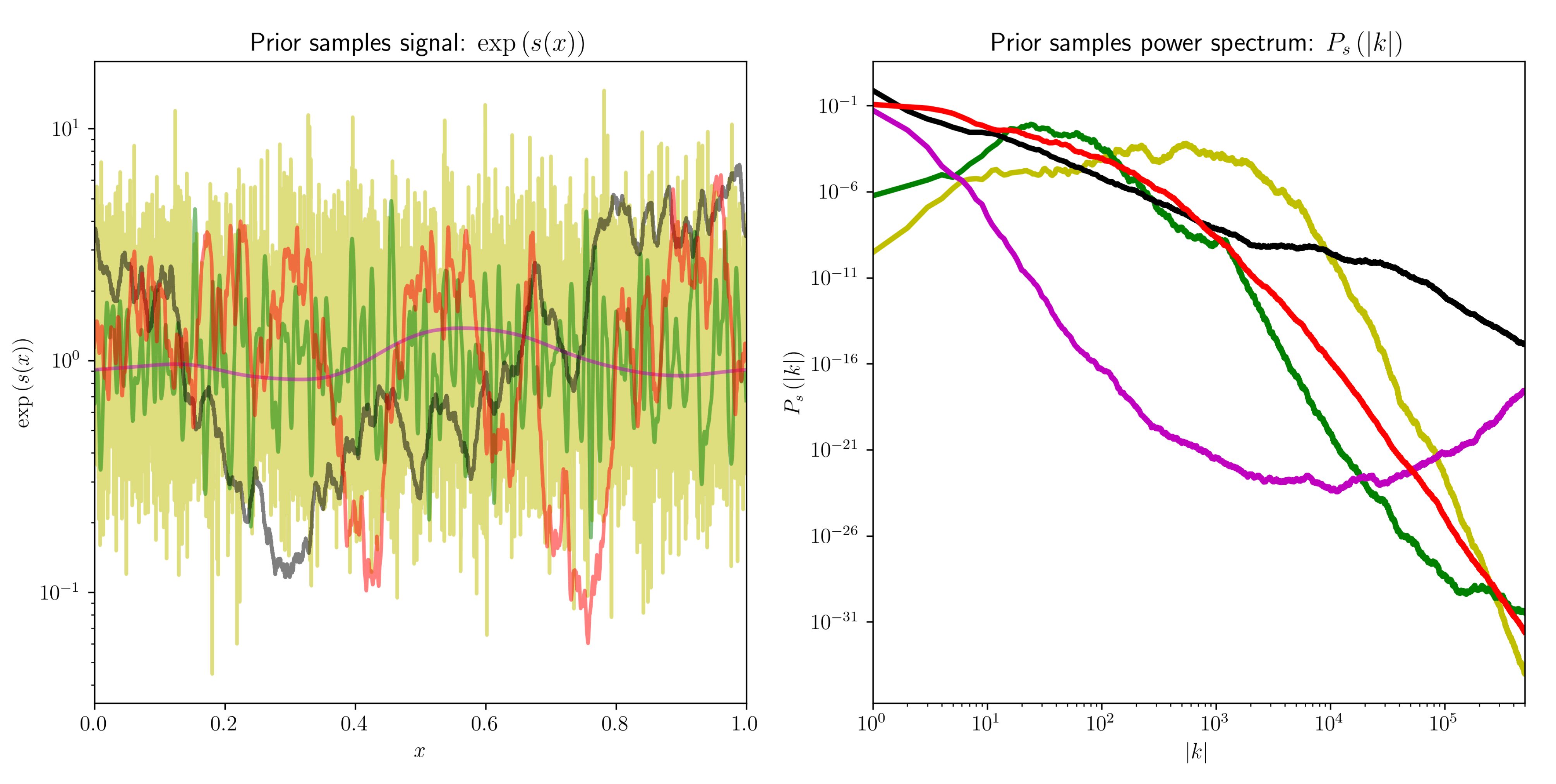
Figure 4.
Random realizations of the joint prior process of the observed signal (left) and corresponding power spectra (right). Matching colors in both panels correspond to samples that belong together. Specifically, each spectrum on the right is randomly generated and the used as the prior power spectrum for a log-normal process to generate the corresponding realizations on the left.

Publisher’s Note: MDPI stays neutral with regard to jurisdictional claims in published maps and institutional affiliations. |
© 2022 by the author. Licensee MDPI, Basel, Switzerland. This article is an open access article distributed under the terms and conditions of the Creative Commons Attribution (CC BY) license (https://creativecommons.org/licenses/by/4.0/).
Share and Cite
MDPI and ACS Style
Frank, P. Geometric Variational Inference and Its Application to Bayesian Imaging. Phys. Sci. Forum 2022, 5, 6. https://doi.org/10.3390/psf2022005006
AMA Style
Frank P. Geometric Variational Inference and Its Application to Bayesian Imaging. Physical Sciences Forum. 2022; 5(1):6. https://doi.org/10.3390/psf2022005006
Chicago/Turabian StyleFrank, Philipp. 2022. "Geometric Variational Inference and Its Application to Bayesian Imaging" Physical Sciences Forum 5, no. 1: 6. https://doi.org/10.3390/psf2022005006