
Quantum Finite Automata and Quiver Algebras †

Department of Mathematics and Statistics, Boston University, 111 Cummington Mall, Boston, MA 02215, USA
*
Author to whom correspondence should be addressed.
†
Presented at the 41st International Workshop on Bayesian Inference and Maximum Entropy Methods in Science and Engineering, Paris, France, 18–22 July 2022.
Phys. Sci. Forum 2022, 5(1), 32; https://doi.org/10.3390/psf2022005032
Published: 14 December 2022
(This article belongs to the Proceedings of The 41st International Workshop on Bayesian Inference and Maximum Entropy Methods in Science and Engineering)
Abstract
:We find an application in quantum finite automata for the ideas and results of [JL21] and [JL22]. We reformulate quantum finite automata with multiple-time measurements using the algebraic notion of a near-ring. This gives a unified understanding towards quantum computing and deep learning. When the near-ring comes from a quiver, we have a nice moduli space of computing machines with a metric that can be optimized by gradient descent.
1. Motivation: QFA and Near-Ring
In quantum theory, the evolution of states is unitary. An observable is modeled by a self-adjoint operator whose eigenvalues are the possible output values, and whose eigenvectors form an orthonormal basis of the state space. As a result, a typical quantum model simply consists of linear operators that form an algebra.
However, when passing from the quantum world to the real world, an actual probabilistic projection to an eigenstate is necessary. Such a probabilistic operation destroys the linear structure, so we need a non-linear (meaning non-distributive) algebraic structure to accommodate such operators. In the 20th century, there were several attempts to solve this problem. See for instance [1,2], and [3] (Chapter 3) for a nice survey. In particular, Pascual Jordan attempted to use near-ring for quantum mechanics.
Let us consider the scenario of quantum computing.
Definition 1
([4]). A quantum finite automata (QFA) is a tuple where:
- 1
- V is a finite set of states which generate the Hilbert space ;
- 2
- is a set of final or accept states;
- 3
- the initial state which is a unit vector in ;
- 4
- Σ is a finite set called the alphabet;
- 5
- For each , is a unitary operator on .
An input to a QFA consists of a word w in the alphabet of the form where for all i. w acts on the initial state of the QFA by , where is the matrix , and is the row vector presentation of . The probability that word w will end in an accept state is
where is the projection from to subspace spanned by F.
Please note that the above definition has not taken the probabilistic projection into account. We make the following reformulation.
Definition 2.
A quantum computing machine is a tuple , where
- 1
- is a Hermitian vector space;
- 2
- equipped with the standard metric, which is called the framing space;
- 3
- is an isometric embedding;
- 4
- is a unitary representation of a group G.
- 5
- is a probabilistic projection.
Ignoring the last item (5) for the moment, this coincides with Definition 1 by setting , the free group generated by a set , and fixing an initial vector .
Here, we treat as a vector space of its own and take an isometric embedding , rather than directly identifying as a subspace in . The state space is treated as an abstract vector space without a preferred basis, while is equipped with a fixed basis that has a real physical meaning (like up/down spinning of an electron). The framing map is interpreted as a bridge between the classical and the quantum world; the image of the fixed basis under e determines a subset of pure state vectors of a certain observable. The adjoint is an orthogonal projection. In the next section, e is no longer required to be an embedding when we consider non-unitary generalizations for machine learning.
For the last item (5), the probabilistic projection can be modeled by a probability space. Specifically, consider a -family of random variables
where is a probability space (that has a probability measure), with the assumption that for every , where denotes the j-th basic vector. Then .
The major additional ingredients in Definition 2, compared to Definition 1, are and . Please note that they are not yet included in the machine language, which is currently the group G. Since e and are not invertible, we cannot enlarge G to include e nor as a group.
To remedy this, first note that (4) can be replaced with an algebra rather than a group, which exhibits linearity and allows not being invertible. Specifically, we require instead:
- (4’)
- is an algebra homomorphism for an algebra A (with unit ).
For instance, A can be the free algebra generated by a set .
With such a modification, we can easily include the framing e and into our language by taking the augmented algebra
where R is generated by the relations for any . The unit of is .
However, we cannot further enlarge to include as an algebra. The reason for this is that always maps to unit vectors and cannot be linear:
To extend by which models actual quantum measurement, we need the notion of a near-ring. It is a set A with two binary operations +, ∘ such that A is a group under `+’, `∘’ is associative, and right multiplication is distributive over addition: for all (but left multiplication is not required distributive: ).
Define to be the near-ring
This near-ring can be understood as the language that controls quantum computing machines. Elements of can be recorded as rooted trees. An example is where . See also the tree on the left-hand side of Figure 1.
The advantage of putting all the algebraic structures into a single near-ring is that we can consider all the quantum computing machines (mathematically -modules) controlled by a single near-ring at the same time. An element of is a quantum algorithm, which can run in all quantum computers controlled by .
2. Near-Ring and Differential Forms
In the setting of Definition 1 and Example 1, it is natural to relax the representations from unitary groups to matrix algebras . Moreover, the quantum measurement can also be simulated by a non-linear function (called activation function). Such a modification will produce a computational model of deep learning.
Definition 3.
An activation module consists of:
- 1
- A noncommutative algebra A and vector space V, F;
- 2
- A family of metrics on V over the space of framed A-moduleswhich is G-equivariant where ;
- (3)
- A collection of possibly non-linear functions
As in (1), we take the augmented algebra which produces linear computations in all framed A-modules simultaneously. With item (3), elements in the near-ring
induce non-linear functions on F, and so they are called non-linear algorithms. An example of how induces non-linear functions on F upon fixing a point in R is given in Example 1.
is understood as a family of computing machines: a point in R fixes how acts on V and the framing map , and hence entirely determines how an algorithm runs in the machine corresponding to .
Let us emphasize that the state space V is basis-free. The family of metrics is -equivariant: for any . Thus, given , the non-linear functions that a induces for the two machines and equal to each other. In other words, an algorithm drives all machines parametrized by the moduli stack to produce functions on F:
As mentioned above, the advantage is that the single near-ring controls all machines in and for all V simultaneously (independent of ).
In [5], we formulated noncommutative differential forms on a near-ring , which induce -valued differential forms on the moduli . It is extended from the Karoubi-de Rham complex [6,7,8,9] for algebras to near-rings. (2) above is the special case for 0-forms, which are simply elements in . The cases of 0-forms and 1-forms are particularly important for gradient descent: recall that gradient of a function is the metric dual of the differential of that function.
Theorem 1
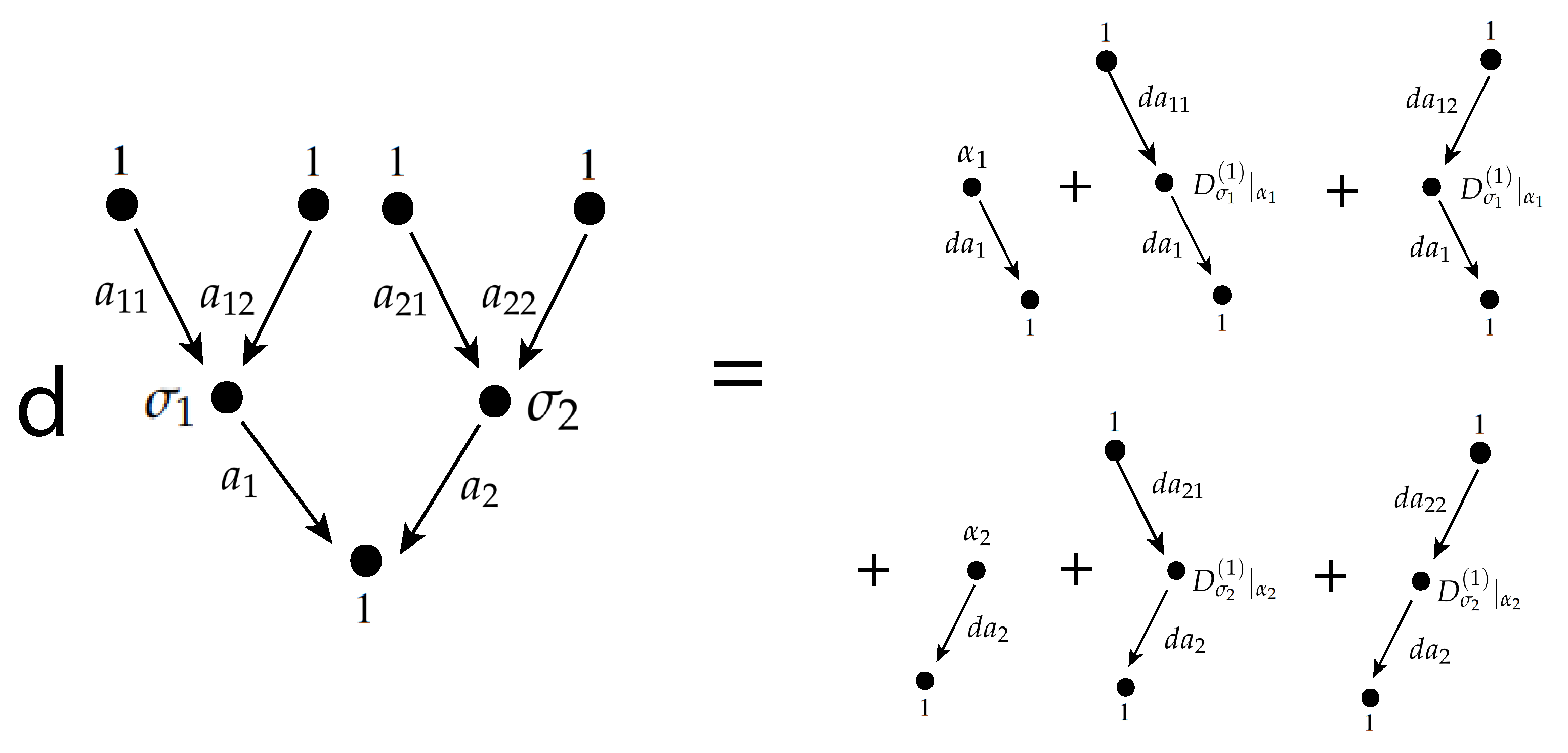
A differential form on can be recorded as a form-valued tree, see the right-hand side of Figure 1. They are rooted trees whose edges are labeled by ; leaves are labeled by ; the root is labeled by 1 (if not a leaf); nodes which are neither leaves nor the root are labeled by the symbols that correspond to the p-th order symmetric differentials of .
In application to machine learning, an algorithm induces a 0-form of , for instance
for a given dataset encoded as a function . This 0-form and its differential induces the cost function and its differential on , respectively, which are the central objects in machine learning.
The differential forms are G-equivariant by construction. There have been a lot of recent works in learning for input data set that has Lie group symmetry [10,11,12,13,14,15,16]. On the other hand, our work has focused on the internal symmetry of the computing machine.
In general, the existence of fine moduli is a big problem in mathematics: the moduli stack may be singular and pose difficulties in applying gradient descent. Fortunately, if A is a quiver algebra, its moduli space of framed quiver representations is a smooth manifold (with respect to a chosen stability condition) [17]. This leads us to deep learning explained in the next section.
3. Deep Learning over the Moduli Space of Quiver Representations
An artificial neural network (see Figure 2 for a simple example) consists of:
- a graph , where is a (finite) set of vertices (neurons) and is a (finite) set of arrows starting and ending in vertices in (transmission between neurons);
- a quiver representation of Q, which associates a vector space to each vertex i and a linear map (called weights) to each arrow a. We denote by and the tail and head of an arrow a, respectively.
- a non-linear function for each vertex i (called an activation function for the neuron).
Activation functions are an important ingredient for neural network; on the other hand, it rarely appears in quiver theory. Its presence allows the neural network to produce non-linear functions.
Remark 1.
In the recent past there has been rising interest in the relations between machine learning and quiver representations [5,18,19,20]. Here, we simply put quiver representation as a part of the formulation of an artificial neural network.
In many applications, the dimension vector is set to be , i.e., all vector spaces associated with the vertices are one-dimensional. For us, it is an unnecessary constraint, and we allow to be any fixed integer vector.
Any non-trivial non-linear function cannot be -equivariant. However, in quiver theory, is understood as a basis-free vector space and requires -equivariance. We resolve this conflict between neural network and quiver theory in [19] using framed quiver representations. The key idea is to put the non-linear function on the framing rather than on the basis-free vector spaces .
Combining with the setting of the last section (Definition 2), we take:
- , the quiver algebra. Elements are formal linear combinations of paths in Q (including the trivial paths at vertices), and product is given by concatenation of paths.
- , the direct sum of all vector spaces over vertices.
- Each vertex is associated with a framing vector space . Then .
- Each point is a framed quiver representation. Specifically, associates a matrix to each arrow a of Q; are the framing linear maps.
- The group G is taken to be . An element acts on R by
- We have (possibly non-linear) maps for each vertex. To match the notation of Definition 2, can be taken as maps by extension by zero.
By the celebrated result of [17], we have a fine moduli space of framed quiver representations , where are the dimension vectors for the framing and representation , respectively. In particular, we have the universal vector bundles over , whose fiber over each framed representation is the representing vector space over the vertex i.
plays an important role in our computational model, namely a vector over a point is the state of the i-th neuron in the machine parametrized by .
To fulfill Definition 2 (see Item (2)), we need to equip each with a bundle metric , so that the adjoint makes sense. In [19], we have found a bundle metric that is merely written in terms of the algebra . It means the formula works for (infinitely many) quiver moduli for all dimension vectors of representations simultaneously.
Theorem 2
([19]). For a fixed vertex , let be the row vector whose entries are all the elements of the form such that . Consider
as a map . Then is -equivariant and descends to a Hermitian metric on over .
Example 1.
Consider the network in Figure 2. The quiver has the arrows for (between the input and hidden layers) and (between the hidden and output layers). In application, we consider the algorithm
where and . Please note that the adjoints and are with respect to the metric and , respectively.
is recorded by the activation tree on the left-hand side of Figure 1, for the case . drives any activation module (with this given quiver algebra) to produce a function . For instance, setting the representing dimension to be 1 and taking to be the ReLu function on is a popular choice. Data passes from the leaves to the root, which is called forward propagation.
Figure 1 shows the differential of . This 1-form is given by
where . The terms are obtained by starting at the output node and moving backwards through the activation tree, which is well known as the backpropagation algorithm. Please note that this works on the algebraic level and is not specific to any representation.
induces a -valued 1-form on . We can also easily produce -valued 1-forms, for instance by (3).
For stochastic gradient descent over the moduli , to find the optimal machine, we still need one more ingredient: a metric on , to turn a one-form to a vector field. Very nicely, the Ricci curvature of the metric (4) given above gives a well-defined metric on . So far, all the ingredients involved (namely the algorithm , its differential, the bundle metric and the metric on moduli) are purely written in algebraic symbols and work for moduli spaces in all dimensions simultaneously.
Theorem 3
Example 2.
Let us consider the network of Figure 2 again, with for simplicity. Let . Over the chart where for all , the -equivariance allows us to assume that . Then are trivial for , and so . Let and . We have
4. Uniformization of Metrics over the Moduli
The original formulation of deep learning is over the flat vector space of representations , rather than the moduli space of framed representations which has a semi-positive metric . In [5], we found the following way of connecting our new approach with the original approach by varying the bundle metric in (4).
We shall assume . Let us write the framing map (which is a rectangular matrix) as where is the largest square matrix and is the remaining part. (In applications usually consists of `bias vectors’.) This allows us to rewrite Equation (4) in the following way:
with .
If instead, we set to different values, then will still be G-equivariant, but it may no longer positive definite on the whole space . Motivated by the brilliant construction of dual Hermitian symmetric spaces, we define
Elements are called space-like representations with respect to . If we set , it becomes
and is exactly the flat vector space . This recovers the original Euclidean learning.
On the other hand, setting , we obtain a semi-negative moduli space [5], which is a generalization of the hyperbolic spaces or non-compact dual of Grassmannians. This is a very useful setting as there have been several fascinating works done on machine learning performed over hyperbolic spaces, for example [24,25,26,27].
Remark 3.
The above construction gives a family of metrics parametrized by α. can be interpreted as filtering parameters that encode the importance of the paths γ. It is interesting to compare this with the celebrated attention mechanism. We can build models that use these parameters to filter away noise signals during the learning process. We are investigating the applications in transfer learning, especially in situations where we only have a small sample of representative data.
Author Contributions
Conceptualization, G.J. and S.-C.L.; writing—original draft preparation, G.J.; writing—review and editing, S.-C.L.; initializing and advising the overall ideas and structures, S.-C.L. All authors have read and agreed to the published version of the manuscript.
Funding
This research received no external funding.
Institutional Review Board Statement
Not applicable.
Informed Consent Statement
Not applicable.
Data Availability Statement
Not applicable.
Acknowledgments
We would like to acknowledge Bernd Henschenmacher, whose communications with us about historical developments of quantum physics has partially inspired this project.
Conflicts of Interest
The authors declare no conflict of interest.
References
- Jordan, P. Zur Axiomatik der Quanten-Algebra; Verlag der Akademie der Wissenschaften und der Literatur in Mainz, in Komm. F. Steiner Verlag: Mainz, Germany, 1950. [Google Scholar]
- Segal, I. Postulates for General Quantum Mechanics. Ann. Math. 1947, 48, 930. [Google Scholar] [CrossRef]
- Liebmann, M.; Ruhaak, H.; Henschenmacher, B. Non-Associative Algebras and Quantum Physics—A Historical Perspective. arXiv 2019, arXiv:1909.04027. [Google Scholar]
- Moore, C.; Crutchfield, J.P. Quantum automata and quantum grammars. Theor. Comput. Sci. 2000, 237, 275–306. [Google Scholar] [CrossRef] [Green Version]
- Jeffreys, G.; Lau, S.C. Noncommutative Geometry of Computational Models and Uniformization for Framed Quiver Varieties. arXiv 2022, arXiv:2201.05900. [Google Scholar]
- Connes, A. Noncommutative differential geometry. Publ. Math. l’IHÉS 1985, 62, 41–144. [Google Scholar] [CrossRef]
- Cuntz, J.; Quillen, D. Algebra extensions and nonsingularity. J. Am. Math. Soc. 1995, 8, 251–289. [Google Scholar] [CrossRef]
- Ginzburg, V. Lectures on Noncommutative Geometry. arXiv 2005, arXiv:0506603. [Google Scholar]
- Tacchella, A. An introduction to associative geometry with applications to integrable systems. J. Geom. Phys. 2017, 118, 202–233. [Google Scholar] [CrossRef] [Green Version]
- Barbaresco, F. Souriau-Casimir Lie Groups Thermodynamics and Machine Learning. In Geometric Structures of Statistical Physics, Information Geometry, and Learning, SPIGL’20, Les Houches, France, 27–31 July 2021; Springer: Cham, Switzerland, 2021; pp. 53–83. [Google Scholar] [CrossRef]
- Cohen, T.; Welling, M. Group Equivariant Convolutional Networks. In Proceedings of the 33rd International Conference on Machine Learning, New York, NY, USA, 19–24 June 2016; Volume 48, pp. 2990–2999. [Google Scholar]
- Cohen, T.; Geiger, M.; Weiler, M. A General Theory of Equivariant CNNs on Homogeneous Spaces. arXiv 2019, arXiv:1811.02017. [Google Scholar]
- Cohen, T.; Geiger, M.; Koehler, J.; Welling, M. Spherical CNNs. In Proceedings of the ICLR, Vancouver, BC, Canada, 30 April–3 May 2018. [Google Scholar]
- Cohen, T.; Weiler, M.; Kicanaoglu, B.; Welling, M. Gauge Equivariant Convolutional Networks and the Icosahedral CNN. In Proceedings of the International Conference on Machine Learning (ICML), Long Beach, CA, USA, 10–15 June 2019. [Google Scholar]
- Cheng, M.; Anagiannis, V.; Weiler, M.; de Haan, P.; Cohen, T.; Welling, M. Covariance in Physics and Convolutional Neural Networks. arXiv 2019, arXiv:1906.02481. [Google Scholar]
- de Haan, P.; Cohen, T.; Welling, M. Natural Graph Networks. arXiv 2020, arXiv:2007.08349. [Google Scholar]
- King, A. Moduli of representations of finite-dimensional algebras. Q. J. Math. Oxf. Ser. 1994, 45, 515–530. [Google Scholar]
- Armenta, M.A.; Jodoin, P.M. The Representation Theory of Neural Networks. arXiv 2020, arXiv:2007.12213. [Google Scholar] [CrossRef]
- Jeffreys, G.; Lau, S.C. Kähler Geometry of Quiver Varieties and Machine Learning. arXiv 2021, arXiv:2101.11487. [Google Scholar]
- Ganev, I.; Walters, R. The QR decomposition for radial neural networks. arXiv 2021, arXiv:2107.02550. [Google Scholar]
- Reineke, M. Framed quiver moduli, cohomology, and quantum groups. J. Algebra 2008, 320, 94–115. [Google Scholar] [CrossRef] [Green Version]
- Nakajima, H. Instantons on ALE spaces, quiver varieties, and Kac-Moody algebras. Duke Math. J. 1994, 76, 365–416. [Google Scholar] [CrossRef] [Green Version]
- Nakajima, H. Quiver varieties and finite-dimensional representations of quantum affine algebras. J. Am. Math. Soc. 2001, 14, 145–238. [Google Scholar] [CrossRef]
- Nickel, M.; Kiela, D. Poincaré Embeddings for Learning Hierarchical Representations. In Proceedings of the NIPS, Long Beach, CA, USA, 4–9 December 2017. [Google Scholar]
- Ganea, O.E.; Bécigneul, G.; Hofmann, T. Hyperbolic Entailment Cones for Learning Hierarchical Embeddings. arXiv 2018, arXiv:1804.01882. [Google Scholar]
- Sala, F.; Sa, C.D.; Gu, A.; Ré, C. Representation Tradeoffs for Hyperbolic Embeddings. Proc. Mach. Learn. Res. 2018, 80, 4460–4469. [Google Scholar]
- Ganea, O.E.; Bécigneul, G.; Hofmann, T. Hyperbolic Neural Networks. arXiv 2018, arXiv:1805.09112. [Google Scholar]
Figure 1.
An example of the backpropagation algorithm for the network in Figure 2 when .
Figure 1.
An example of the backpropagation algorithm for the network in Figure 2 when .

Figure 2.
A simple neural network with one hidden layer with s-many neurons. Neural networks in applications are typically much more complicated, but in nature are still quiver representations equipped with activation functions.
Figure 2.
A simple neural network with one hidden layer with s-many neurons. Neural networks in applications are typically much more complicated, but in nature are still quiver representations equipped with activation functions.

Publisher’s Note: MDPI stays neutral with regard to jurisdictional claims in published maps and institutional affiliations. |
© 2022 by the authors. Licensee MDPI, Basel, Switzerland. This article is an open access article distributed under the terms and conditions of the Creative Commons Attribution (CC BY) license (https://creativecommons.org/licenses/by/4.0/).
Share and Cite
MDPI and ACS Style
Jeffreys, G.; Lau, S.-C. Quantum Finite Automata and Quiver Algebras. Phys. Sci. Forum 2022, 5, 32. https://doi.org/10.3390/psf2022005032
AMA Style
Jeffreys G, Lau S-C. Quantum Finite Automata and Quiver Algebras. Physical Sciences Forum. 2022; 5(1):32. https://doi.org/10.3390/psf2022005032
Chicago/Turabian StyleJeffreys, George, and Siu-Cheong Lau. 2022. "Quantum Finite Automata and Quiver Algebras" Physical Sciences Forum 5, no. 1: 32. https://doi.org/10.3390/psf2022005032