Particle Physics at Primary Schools: A Report on the Italian Project ^†

Abstract

Dynamics of many classical physics systems are described in terms of Hamilton’s equations. Commonly, initial conditions are only imperfectly known. The associated volume in phase space is preserved over time due to the symplecticity of the Hamiltonian flow. Here we study the propagation of uncertain initial conditions through dynamical systems using symplectic surrogate models of Hamiltonian flow maps. This allows fast sensitivity analysis with respect to the distribution of initial conditions and an estimation of local Lyapunov exponents (LLE) that give insight into local predictability of a dynamical system. In Hamiltonian systems, LLEs permit a distinction between regular and chaotic orbits. Combined with Bayesian methods we provide a statistical analysis of local stability and sensitivity in phase space for Hamiltonian systems. The intended application is the early classification of regular and chaotic orbits of fusion alpha particles in stellarator reactors. The degree of stochastization during a given time period is used as an estimate for the probability that orbits of a specific region in phase space are lost at the plasma boundary. Thus, the approach offers a promising way to accelerate the computation of fusion alpha particle losses.

1. Introduction

Hamilton’s equations describe the dynamics of many classical physics systems such as classical mechanics, plasma physics or electrodynamics. In most of these cases, chaos plays an important role [1]. One fundamental question in analyzing these chaotic Hamiltonian systems is the distinction between regular and chaotic regions in phase space. A commonly used tool are Poincaré maps, which connect subsequent intersections of orbits with a lower-dimensional subspace, called Poincaré section. For example, in a planetary system one could record a section each time the planet has made a turn around the Sun. The resulting pattern of intersection points on this subspace allow insight into the dynamics of the underlying system: regular orbits stay bound to a closed hyper-surface and do not leave the confinement volume, whereas chaotic orbits might spread over the whole phase space. This is related to the breaking of KAM (Kolmogorov-Arnold-Moser) surfaces that form barriers for motion in phase space [2]. The classification of regular versus chaotic orbits is performed, e.g., via box-counting [3] or by calculating the spectrum of Lyapunov exponents [4,5,6]. Lyapunov exponents measure the asymptotic average exponential rate of divergence of nearby orbits in phase space over infinite time and are therefore invariants of the dynamical system. When considering only finite time, the obtained local Lyapunov exponents (LLEs) for a specific starting position depend on the position in phase space and give insight into the local predictability of the dynamical system of interest [7,8,9,10]. Poincaré maps are in most cases inefficient to compute as their computation involves numerical integration of Hamilton’s equations even though only intersections with the surface of interest are recorded. When using a surrogate model to interpolate the Poincaré map, the symplectic structure of phase space arising from the description in terms of the Hamiltonian description has to be preserved to obtain long-term stability and conservation of invariants of motion, e.g., volume preservation. Additional information on Hamiltonian systems and symplecticity can be found in [2,11]. Here, we use a structure-preserving Gaussian process surrogate model (SympGPR) that interpolates directly between Poincaré sections and thus avoids unnecessary computation while achieving similar accuracy as standard numerical integration schemes [12].

In the present work, we investigate how the symplectic surrogate model [12] can be used for early classification of chaotic versus regular trajectories based on the calculation of LLEs. The latter are calculated using the Jacobian that is directly available from the surrogate model [13]. As LLEs also depend on time, we study their distribution on various time scales to estimate the needed number of mapping iterations. We combine the orbit classification with a sensitivity analysis based on variance decomposition [14,15,16] to evaluate the influence of uncertain initial conditions in different regions of phase space. The analysis is carried out on the well-known standard map [17] that is well suited for validation purposes as a closed form expression for the Poincaré maps is available. This, however, does not influence the performance of the surrogate model that is applicable also in cases where such a closed form doesn’t exist [12].

The intended application is the early classification of regular and chaotic orbits of fusion alpha particles in stellarator reactors [3]. While regular particles can be expected to remain confined indefinitely, only chaotic orbits have to be traced to the end. This offers a promising way to accelerate loss computations for stellarator optimization.

2. Methods

2.1. Hamiltonian Systems

A $f-$dimensional system (with $2f-$dimensional phase space) described by its Hamiltonian $H(\mathit{q},\mathit{p},t)$ depending on f generalized coordinates $\mathit{q}$ and f generalized momenta $\mathit{p}$ satisfies Hamilton’s canonical equations of motion,

$$\begin{array}{c}\hfill \dot{\mathit{q}}\left(t\right)=\frac{d\mathit{q}\left(t\right)}{dt}={\nabla }_{\mathit{p}}H(\mathit{q}\left(t\right),\mathit{p}\left(t\right)),\dot{\mathit{p}}\left(t\right)=\frac{d\mathit{p}\left(t\right)}{dt}=-{\nabla }_{\mathit{q}}H(\mathit{q}\left(t\right),\mathit{p}\left(t\right)),\end{array}$$

(1)

which represent the time evolution as integral curves of the Hamiltonian vector field.

Here, we consider the standard map [17] that is a well-studied model to investigate chaos in Hamiltonian systems. Each mapping step corresponds to one Poincaré map of a periodically kicked rotator:

$$\begin{array}{c}\hfill p_{n+1}=(p_n+K\sin \left(q_n\right))\mathrm{mod}2\pi ,q_{n+1}=(q_n+p_{n+1})\mathrm{mod}2\pi ,\end{array}$$

(2)

where K is the stochasticity parameter corresponding to the intensity of the perturbation. The standard map is an area-preserving map with $\det J=1$, where J is its Jacobian:

$$J=\left(\begin{array}{cc}\frac{\partial q_{n+1}}{\partial q_n}& \frac{\partial q_{n+1}}{\partial p_n}\\ \frac{\partial p_{n+1}}{\partial q_n}& \frac{\partial p_{n+1}}{\partial p_n}\end{array}\right)=\left(\begin{array}{cc}1+K\cos \left(q_n\right)& 1\\ K\cos \left(q_n\right)& 1\end{array}\right)$$

(3)

2.2. Symplectic Gaussian Process Emulation

A Gaussian process (GP) [18] is a collection of random variables, any finite number of which have a joint Gaussian distribution. A GP is fully specified by its mean $\mathit{m}\left(\mathit{x}\right)$ and kernel or covariance function $K(\mathit{x},{\mathit{x}}^{\prime })$ and is denoted as

$$\mathit{f}\left(\mathit{x}\right)\sim \mathcal{GP}(\mathit{m}\left(\mathit{x}\right),K(\mathit{x},{\mathit{x}}^{\prime })),$$

(4)

for input data points $\mathit{x}\in {\mathbb{R}}^d$. Here, we allow vector-valued functions $\mathit{f}\left(\mathit{x}\right)\in {\mathbb{R}}^D$ [19]. The covariance function is a positive semidefinite matrix-valued function, whose entries ${\left(K(\mathit{x},{\mathit{x}}^{\prime })\right)}_{ij}$ express the covariance between the output dimensions i and j of $\mathit{f}\left(\mathit{x}\right)$.

For regression, we rely on observed function values $Y\in {\mathbb{R}}^{D\times N}$ with entries $\mathit{y}=\mathit{f}\left(\mathit{x}\right)+ϵ$. These observations may contain local Gaussian noise $ϵ$, i.e., the noise is independent at different positions $\mathit{x}$ but may be correlated between components $\mathit{y}$. The input variables are aggregated in the $d\times N$ design matrix X, where N is the number of training data points. The posterior distribution, after taking training data points into account, is still a GP with updated mean $F_{*}\equiv \mathbb{E}\left(F\left(X_{*}\right)\right)$ and covariance function allowing to make predictions for test data $X_{*}$:

$$\begin{array}{cc}\hfill F_{*}& =K(X_{*},X){(K(X,X)+{\mathsf{\Sigma }}_n)}^{-1}Y,\hfill \end{array}$$

(5)

$$\begin{array}{cc}\hfill \mathrm{cov}\left(F_{*}\right)=& \begin{array}{c}K(X_{*},X_{*})-K(X_{*},X){(K(X,X)+{\mathsf{\Sigma }}_n)}^{-1}K(X,X_{*}),\hfill \end{array}\hfill \end{array}$$

(6)

where ${\mathsf{\Sigma }}_n\in {\mathbb{R}}^{ND\times ND}$ is the covariance matrix of the multivariate output noise for each training data point. Here we use the shorthand notation $K(X,X)$ for the block matrix assembled over the output dimension D in addition to the number of input points as in a single-output GP with a scalar covariance function $k(\mathit{x},{\mathit{x}}^{\prime })$ that expresses the covariance of different input data points $\mathit{x}$ and ${\mathit{x}}^{\prime }$. The kernel parameters are estimated given the input data by minimizing the negative log-likelihood [18].

To construct a GP emulator that interpolates symplectic maps for Hamiltonian systems, symplectic Gaussian process regression (SympGPR) was presented in [12] where the generating function $F(q,P)$ and its gradients are interpolated using a multi-output GP with derivative observations [20,21]. The generating function links old coordinates $(q,p)=(q_n,p_n)$ to new coordinates $(Q,P)=(q_{n+1},p_{n+1})$ (e.g., after one iteration of the standard map Equation (2)) via a canonical transformation such that the symplectic property of phase space is preserved. Thus, input data points consist of pairs $(q,P)$. Then, the covariance matrix contains the Hessian of an original scalar covariance function $k(q,P,q^{\prime },P^{\prime })$ as the lower block matrix $L(q,P,q^{\prime },P^{\prime })$ (denoted with the red box):

(7)

Using the algorithm for the (semi-)implicit symplectic GP map as presented in [12], once the SympGPR model is trained and the covariance matrix calculated, the model is used to predict subsequent time steps or Poincaré maps for arbitrary initial conditions.

For the estimation of the Jacobian (Equation (3)) from the SympGPR, the Hessian of the generating function $F(q,P)$ has to be inferred from the training data. Thus, the covariance matrix is extended with a block matrix C containing third derivatives of $k(q,P,q^{\prime },P^{\prime })$:

$$C=\left(\begin{array}{cccc}{\partial }_{q,q^{\prime },q}k& {\partial }_{q,P^{\prime },q}k& {\partial }_{P,q^{\prime },q}k& {\partial }_{P,P^{\prime },q}k\\ {\partial }_{q,q^{\prime },P}k& {\partial }_{q,P^{\prime },P}k& {\partial }_{P,q^{\prime },P}k& {\partial }_{P,P^{\prime },P}k\end{array}\right).$$

(8)

The mean of the posterior distribution of the desired Hessian of the generating function $F(q,P)$ is inferred via

$${\nabla }^{2}F={({\partial }_{qq}^{2}F,{\partial }_{qP}^{2}F,{\partial }_{Pq}^{2}F,{\partial }_{PP}^{2}F)}^{\top }=C{L}^{-1}Y.$$

(9)

As we have a dependence on mixed coordinates $Q(\overline{q}(q,p),P(q,p))$ and $P(Q(q,p),\overline{p}(q,p))$, where we used $\overline{q}(q,p)=q$ and $\overline{p}(q,p)=p$ to correctly carry out the inner derivatives, the needed elements for the Jacobian can be calculated employing the chain rule. The Jacobian is then given as the solution of the well-determined linear set of equations:

$$\begin{array}{c}\hfill \frac{\partial Q}{\partial q}=\frac{\partial Q}{\partial \overline{q}}\frac{\partial \overline{q}}{\partial q}+\frac{\partial Q}{\partial P}\frac{\partial P}{\partial q},\frac{\partial Q}{\partial p}=\frac{\partial Q}{\partial \overline{q}}\frac{\partial \overline{q}}{\partial p}+\frac{\partial Q}{\partial P}\frac{\partial P}{\partial p},\end{array}$$

(10)

$$\begin{array}{c}\hfill \frac{\partial P}{\partial q}=\frac{\partial P}{\partial Q}\frac{\partial Q}{\partial q}+\frac{\partial P}{\partial \overline{p}}\frac{\partial \overline{p}}{\partial q},\frac{\partial P}{\partial p}=\frac{\partial P}{\partial Q}\frac{\partial Q}{\partial p}+\frac{\partial P}{\partial \overline{p}}\frac{\partial \overline{p}}{\partial p},\end{array}$$

(11)

where we use the following correspondence to determine all factors of the SOEs:

$$\left(\begin{array}{cc}\frac{\partial Q}{\partial \overline{q}}& \frac{\partial Q}{\partial P}\\ \frac{\partial \overline{p}}{\partial \overline{q}}& \frac{\partial \overline{p}}{\partial P}\end{array}\right)={\left(\begin{array}{cc}\frac{\partial \overline{q}}{\partial Q}& \frac{\partial P}{\partial Q}\\ \frac{\partial \overline{q}}{\partial \overline{p}}& \frac{\partial P}{\partial \overline{p}}\end{array}\right)}^{\top }=\left(\begin{array}{cc}1+\frac{{\partial }^{2}F}{\partial q\partial P}& -\frac{{\partial }^{2}F}{\partial P\partial P}\\ -\frac{{\partial }^{2}F}{\partial q\partial q}& 1+\frac{{\partial }^{2}F}{\partial P\partial q}\end{array}\right).$$

(12)

2.3. Sensitivity Analysis

Variance-based sensitivity analysis decomposes the variance of the model output into portions associated with uncertainty in the model inputs or initial conditions [14,15]. Assuming independent input variables $X_i$, $i=1,...,d$, the functional analysis of variance (ANOVA) allows a decomposition of the scalar model output Y from which the decomposition of the variance can be deduced:

$$V\left[Y\right]=\sum _{i=1}^d{V}_i+\sum _{1\le i<j\le d}{V}_{ij}+...+V_{1,2,...,d}$$

(13)

The first term describes the variation in variance only due to changes in single variables $X_i$, whereas higher-order interactions are depicted in the contributions of the interaction terms. From this, first-order Sobol’ indices $S_i$ are defined as the corresponding fraction of the total variance, whereas total Sobol’ indices $S_{T_i}$ also take the influence of $X_i$ interacting with other input variables into account [14,15]:

$$S_i=\frac{V_i}{\mathrm{Var}\left(Y\right)},S_{T_i}=\frac{E_{{\mathit{x}}_{\sim i}}({\mathrm{Var}}_{X_i}\left(Y\right|{\mathit{x}}_{\sim i})}{\mathrm{Var}\left(Y\right)}$$

(14)

Several methods for efficiently calculating Sobol’ indices have been presented, e.g., MC sampling [14,16] or direct estimation from surrogate models [22,23]. Here, we use the MC sampling strategy presented in [16] using two sampling matrices $\mathit{A},\mathit{B}$ and a combination of both ${\mathit{A}}_{\mathit{B}}^{\left(i\right)}$, where all columns are from $\mathit{A}$ except the i-th column which is from $\mathit{B}$:

$$S_i\mathrm{Var}\left(Y\right)=\frac{1}{N}\sum _{i=1}^{N}f{\left(\mathit{B}\right)}_j(f{\left({\mathit{A}}_B^{\left(i\right)}\right)}_j-f{\left(\mathit{A}\right)}_j),S_{T_i}\mathrm{Var}\left(Y\right)=\frac{1}{2N}\sum _{i=1}^N{(f{\left(\mathit{A}\right)}_j-f{\left({\mathit{A}}_B^{\left(i\right)}\right)}_j)}^2,$$

(15)

where f denotes the model to be evaluated.

2.4. Local Lyapunov Exponents

For a dynamical system in ${\mathbb{R}}^D$, D Lyapunov characteristic exponents ${\lambda }_n$ give the exponential separation of trajectories with initial conditions $z\left(0\right)=\left(q\right(0),p(0\left)\right)$ of a dynamical system with perturbation $\delta z$ over time:

$$\left|\delta z\left(T\right)\right|={\mathcal{J}}_{z\left(T\right)}^{\left(T\right)}\delta z\left(0\right)\approx e^{T\lambda }\left|\delta z\left(0\right)\right|,$$

(16)

where ${\mathcal{J}}_{z\left(T\right)}^{\left(T\right)}$ is a time-ordered product of Jacobians ${\mathcal{J}}_{z(T-1)}{\mathcal{J}}_{z(T-2)}...{\mathcal{J}}_{z\left(1\right)}{\mathcal{J}}_{z\left(0\right)}$ [4]. The Lyapunov exponents are then given as the logarithm of the eigenvalues of the positive and symmetric matrix.

$${\displaystyle \mathsf{\Lambda }=\underset{T\to \infty }{lim}{\left[{\mathcal{J}}_{z\left(T\right)}^{\left(T\right)\top }{\mathcal{J}}_{z\left(T\right)}^{\left(T\right)}\right]}^{1/\left(2T\right)},}$$

(17)

where ⊤ denotes the transpose of ${\mathcal{J}}_{z\left(T\right)}^{\left(T\right)}$.

For a D-dimensional system, there exist D Lyapunov exponents ${\lambda }_n$ giving the rate of growth of a D-volume element with ${\lambda }_1+...+{\lambda }_D$ corresponding to the rate of growth of the determinant of the Jacobian $\det \left({\mathcal{J}}_{z\left(T\right)}^{\left(T\right)}\right)$. From this follows that for a Hamiltonian system with a symplectic (e.g., volume-preserving) phase space structure, Lyapunov exponents exist in additive inverse pairs as the determinant of the Jacobian is constant, ${\lambda }_1+...+{\lambda }_D$ = 0. In the dynamical system of the standard map with $D=2$ considered here, the Lyapunov exponents allow a distinction between regular and chaotic motion. If the Lyapunov exponents ${\lambda }_1=-{\lambda }_2>0$, neighboring orbits separate exponentially which corresponds to a chaotic region. In contrast, when ${\lambda }_1=-{\lambda }_2\approx 0$ the motion is regular [1].

As the product of Jacobians is ill-conditioned for large values of T, several algorithms have been proposed to calculate the spectrum of Lyapunov exponents [13]. Here, we determine local Lyapunov exponents (LLE) that determine the predictability of an orbit of the system at a specific phase point for finite time. In contrast to global Lyapunov exponents they depend on T and on the position in phase space $z$. We use recurrent Gram-Schmidt orthonormalization procedure through QR decomposition [5,6,24], where we follow the evolution of D initially orthonormal deviation vectors ${\mathit{w}}_0^n$. The Jacobian is decomposed into ${\mathcal{J}}_{z\left(0\right)}=Q^{\left(1\right)}{R}^{\left(1\right)}$, where $Q^{\left(1\right)}$ is an orthogonal matrix and $R^{\left(1\right)}$ is an upper triangular matrix yielding a new set of orthonormal vectors ${\mathit{w}}_i$. At the next mapping iteration, the matrix product ${\mathcal{J}}_{z\left(1\right)}{Q}^{\left(1\right)}$ is again decomposed. This procedure is repeated T times to arrive at ${\mathcal{J}}_{z\left(t\right)}^{\left(T\right)}=Q^{\left(T\right)}{R}^{\left(T\right)}{R}^{(T-1)}...R^{\left(0\right)}$. The Lyapunov exponents are then estimated from the diagonal elements of $R^{\left(t\right)}$

$${\lambda }_n=\frac{1}{T}\sum _{t=1}^T\ln R_{nn}^{\left(t\right)}.$$

(18)

3. Results and Discussion

In the following we apply an implicit SympGPR model with a product kernel [12]. Due to the periodic topology of the standard map we use a periodic kernel function to construct the covariance matrix in Equation (7) with periodicity $2\pi$ in q, whereas a squared exponential kernel is used in P:

$$k(q,q_i,P,P_i)={\sigma }_f^2\exp \left(-\frac{{\sin }^2((q-q_i)/2)}{2l_q^2}\right)\exp \left(-\frac{{(P-P_i)}^2}{2l_P^2}\right).$$

(19)

Here ${\sigma }_f^2$ specifies the amplitude of the fit and is set in accordance with the observations to $2\max {\left(\right|Y\left|\right)}^2$, where Y corresponds to the change in coordinates. The hyperparameters $l_q,l_P$ are set to their maximum likelihood value by minimizing the negative log-likelihood given the input data using the L-BFGS-B routine implemented in Python [18]. The noise in observations is set to ${\sigma }_n^2={10}^{-16}$. 30 initial data points are sampled from a Halton sequence to ensure good coverage of the training region in the range $[0,2\pi ]\times [0,2\pi ]$ and Equation (2) is evaluated once to obtain the corresponding final data points. Each pair of initial and final conditions constitutes one sample of the training data set. Once the model is trained, it is used to predict subsequent mapping steps for arbitrary initial conditions and to infer the corresponding Jacobians for the calculation of the local Lyapunov exponents. Here, we consider two test cases of the standard map with different values of the stochasticity parameter $K=0.9$ and $K=2.0$ (Equation (2)). For each of the test cases, a surrogate model is trained. While in the first case the last KAM surface is not yet broken and therefore the region of stochasticity is still confined in phase space, in the latter case the chaotic region covers a much larger portion of phase space. However, there still exist islands of stability with regular orbits [2]. For $K=0.9$ the mean squared error (MSE) for the training data is $1.4\times {10}^{-6}$, whereas the test MSE after one mapping application is found to be $2.4\times {10}^{-6}$. A similar quality of the surrogate model is reached for $K=2.0$, where the training MSE is $1.6\times {10}^{-7}$ and the test MSE $2.4\times {10}^{-7}$.

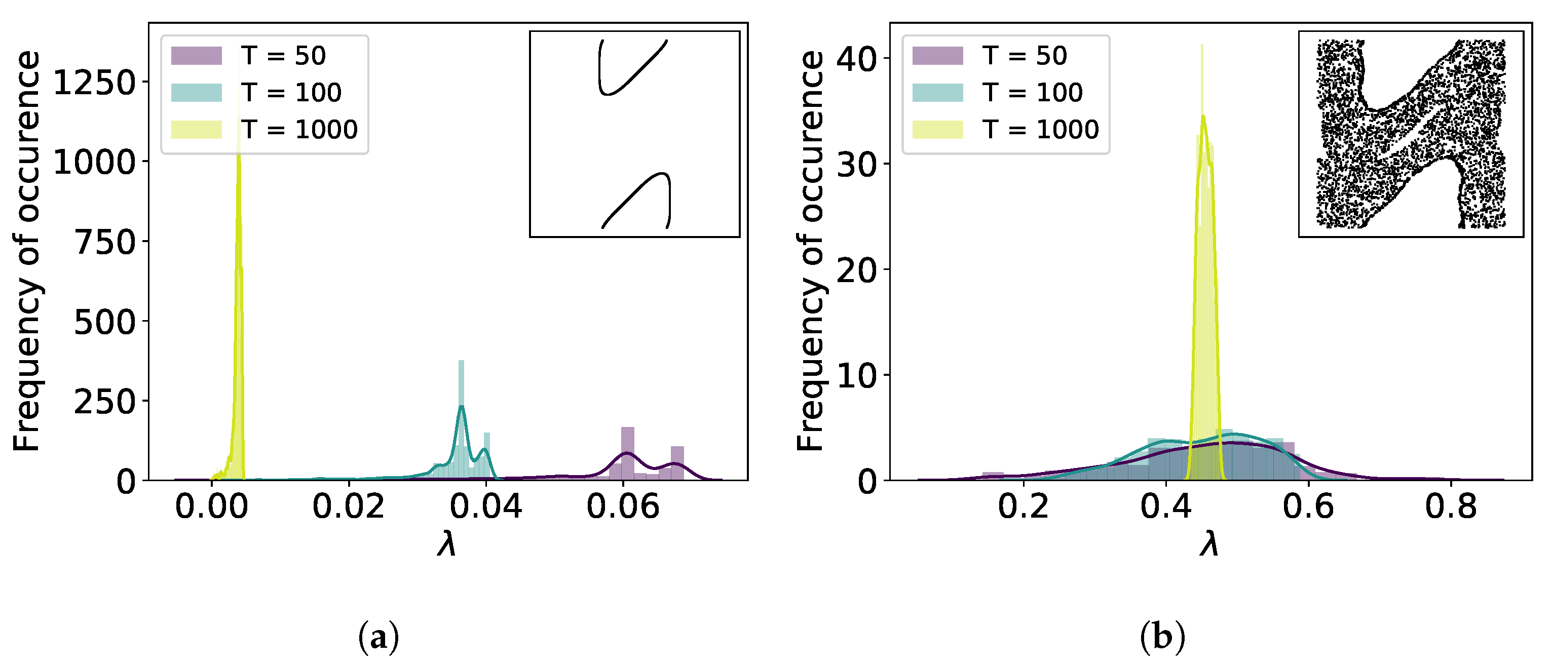
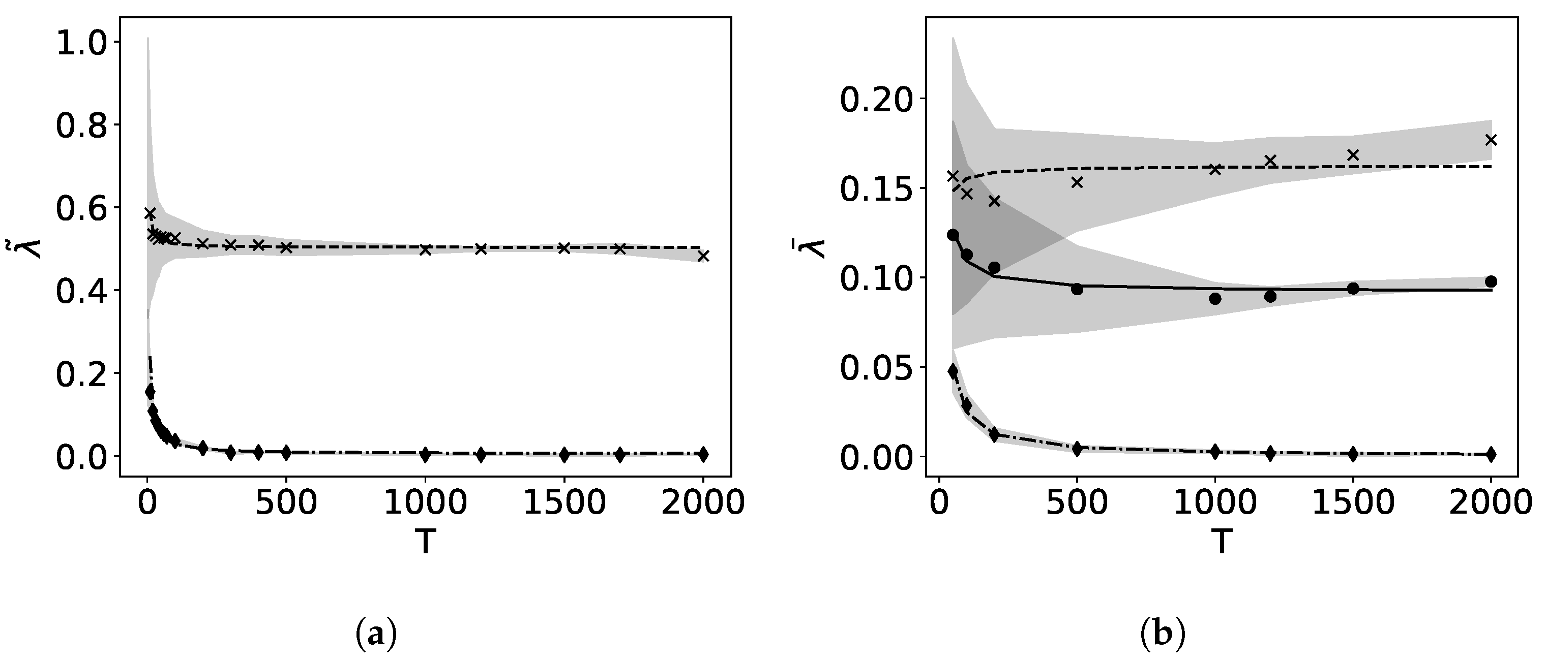
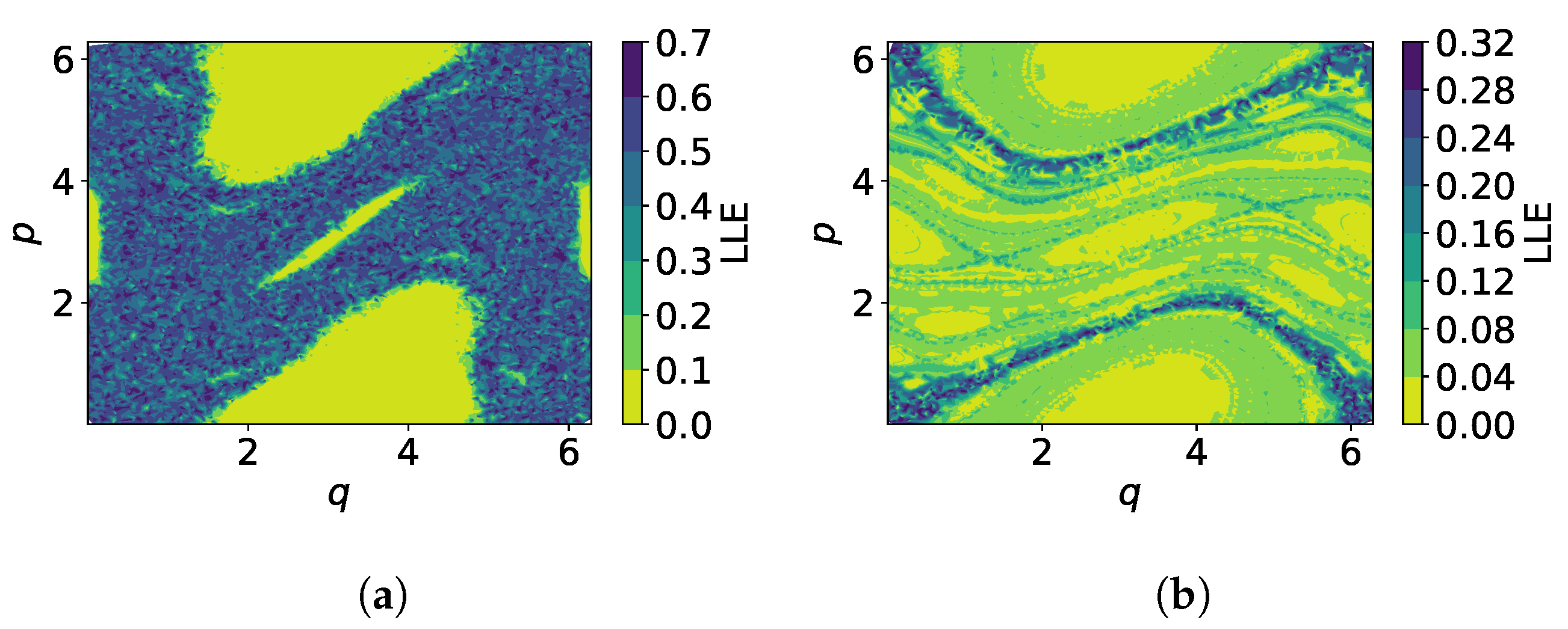
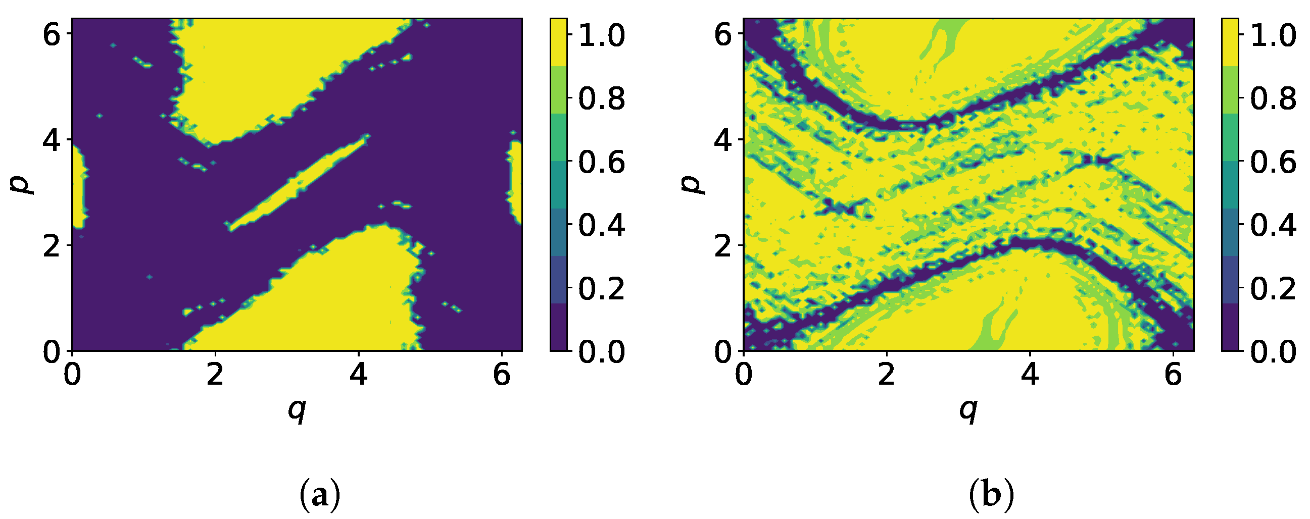
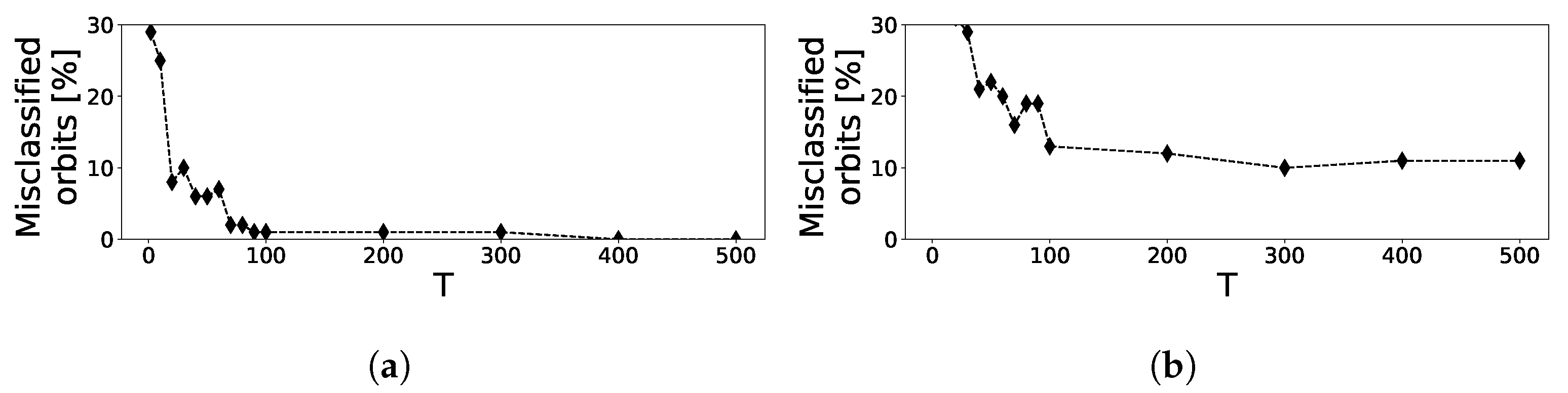
3.1. Local Lyapunov Exponents and Orbit Classification

For the evaluation of the distribution of the local Lyapunov exponents with respect to the number of mapping iterations T and phase space position $z=(q,p)$, 1000 points are sampled from each orbit under investigation. In the following, we only consider the maximum local Lyapunov exponent as it determines the predictability of the system. For each of the 1000 points, the LLEs are calculated using Equation (18), where the needed Jacobians are given by the surrogate model by evaluating Equation (9) and solving Equation (11).

Figure 1 shows the distributions for $K=2.0$, $T=50$, $T=100$ and $T=1000$ for two different initial conditions resulting in a regular and a chaotic orbit. In the regular case the distribution exhibits a sharp peak and with increasing T moves closer to 0. This bias due to the finite number of mapping iterations decreases with $\mathcal{O}(1/T)$ as shown in Figure 2 [25]. For the chaotic orbit, the distribution looks smooth and its median is clearly >0 as expected. For a smaller value of $K=0.9$ the dynamics in phase space exhibit larger variety with regular, chaotic and also weakly chaotic orbits that remain confined in a small stochastic layer around hyperbolic points. Hence, the transition between regular, weakly chaotic and chaotic orbits is continuous due to the larger variety in phase space. For fewer mapping iterations, possible values of $\lambda$ are overlapping, thus preventing a clear distinction between confined chaotic and chaotic orbits.

When considering the whole phase space with 200 orbits with initial conditions sampled from a Halton sequence in the range $[0,\pi ]\times [0,2\pi ]$, already $T=50$ mapping iterations provide insight in the predictability of the standard map (Figure 3). If for a region in phase space the obtained LLE is positive, the predictability in this region is restricted as the instability there is relatively large. If, however, the LLE is close to zero, we can conclude that this region in phase space is governed by regular motion and is therefore highly predictable. For $K=2.0$ the orbits constituting the chaotic sea have large positive LLEs, whereas islands of stability built by regular orbits show LLEs close to 0. A similar behavior can be observed for $K=0.9$, where again regions around stable elliptic points feature $\lambda \approx 0$ while stochastic regions exhibit a varying range of LLEs in accordance to Figure 2.

Based on the estimation of the LLEs, a Gaussian Bayesian classifier [26] is used to determine the probability of an orbit being regular, where we assume that LLEs are normally distributed in each class. First, the classifier is trained on LLEs resulting from 200 different initial conditions for T mapping iterations with the corresponding class labels resulting from the chosen reference being the generalized alignment index (GALI) [27]. Then, ${10}^4$ test orbits are sampled from a regular grid in the range $[0,\pi ]\times [0,2\pi ]$ with $\Delta q=\Delta p=2\pi /10$, their LLE is calculated for T mapping iterations and the orbits are then classified. The results for $K=0.9$ and $K=2.0$ with $T=50$ are shown in Figure 4, where the color map indicates the probability that the test orbit is regular. While for $K=2.0$ the classifier provides a very clear distinction between regular and chaotic regions, the distinction between confined chaotic and regular orbits for $K=0.9$ is less clear. With increasing number of mapping iterations, the number of misclassifications reduces as depicted in Figure 5. If the predicted probability that an orbit belongs to a certain class is lower than $70\%$, the prediction is not accepted and the orbit is marked as misclassified. With $K=0.9$, the percentage of misclassified orbits does not drop below approximately $10\%$, because the transition between regular and chaotic motion is continuous.

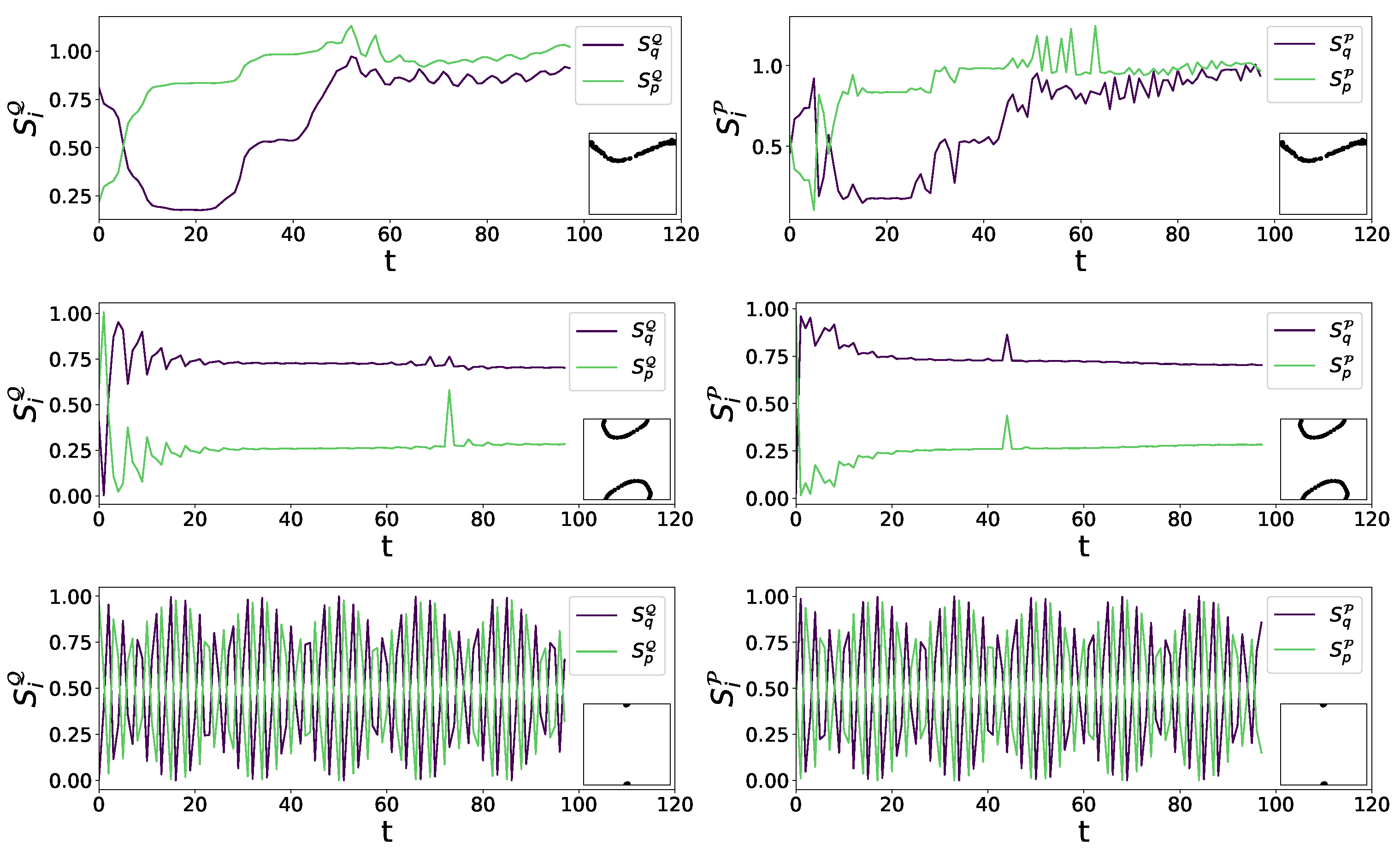
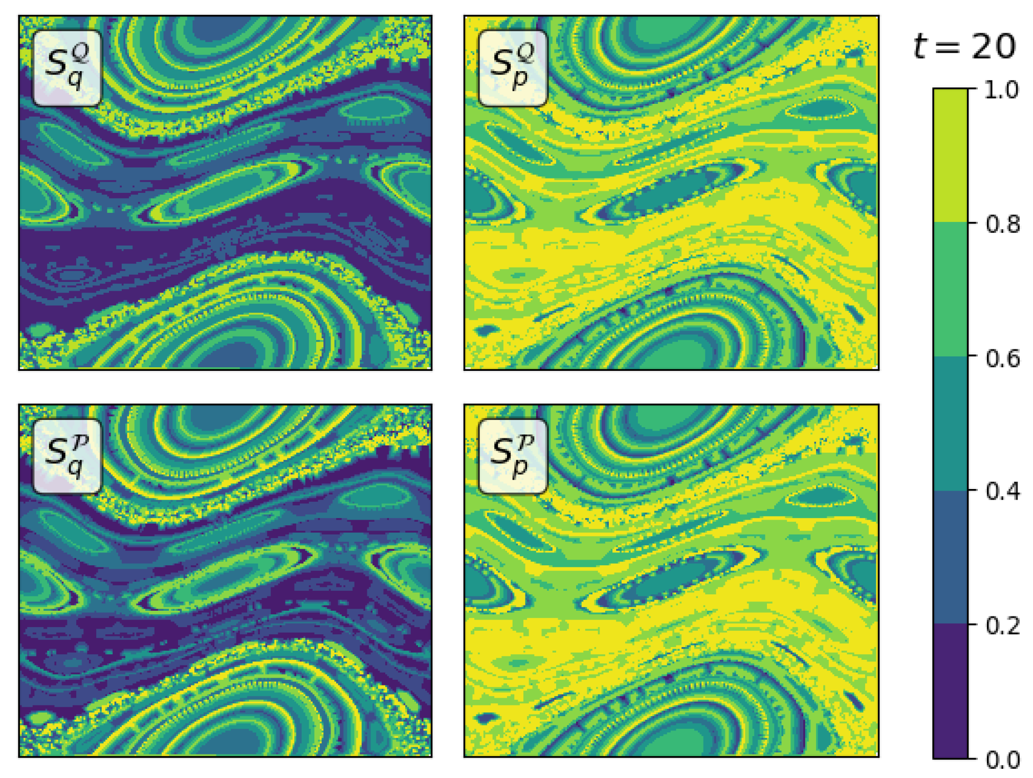
3.2. Sensitivity Analysis

The total Sobol’ indices are calculated for the outputs from the symplectic surrogate model $(Q,P)$ using Equation (15) with $N=2000$ uniformly distributed random points within a box of size $[{10}^{-3}\times {10}^{-3}]$ for each of the $T=100$ mapping iterations as we are interested in the temporal evolution of the indices. For the standard map at $K=0.9$ with $d=2$ input and $D=2$ output dimensions, 4 total Sobol’ indices are obtained: $S_q^Q$ and $S_q^P$ denoting the influence of q and $S_p^Q$ and $S_p^P$ marking the influence of p on the output. We obtain good agreement with an MSE in the order of ${10}^{-6}$ between the indices obtained by the surrogate model and those using reference data.

As shown in Figure 6 for three different initial conditions for $K=0.9$ depending on the orbit type, either chaotic or regular, the sensitivity indices behave differently. In case of a regular orbit close to a fixed point, $S_j^i$ are oscillating, indicating that both input variables have similar influence on average. Getting further from the fixed point, closer to the border of stability, the influence of q gets bigger. This, however, is in contrast to the behavior in the chaotic case, where initially the variance in p has larger influence on the model output. However, when observing the indices over longer periods of time, both variables have similar influence. In Movie S01 in the supplemental material, the time evolution of all four total Sobol’ indices obtained for the standard map are shown in phase space. Each frame is averaged over 10 subsequent mapping iterations. One snapshot is shown in Figure 7. The observation of the whole phase space sustains the findings in Figure 6.

4. Conclusions

We presented an approach for orbit classification in Hamiltonian systems based on a structure preserving surrogate model combined with early classification based on local Lyapunov exponents directly available from the surrogate model. The approach was tested on two cases of the standard map. Depending on the perturbation strength, we either see a continuous transition from regular to chaotic orbits for $K=0.9$ or a sharp separation between those two classes for higher perturbation strengths. This also impacts the classification results obtained from a Bayesian classifier. The presented method is applicable to chaotic Hamiltonian systems and is especially useful when a closed form expression for Poincaré maps is not available. Also, the accompanying sensitivity analysis provides valuable insight: in transition regions between regular and chaotic motion the Sobol’ indices for time-series can be used to analyze the influence of input variables.

References

1. Ott, E. Chaos in Hamiltonian systems. In Chaos in Dynamical Systems, 2nd ed.; Cambridge University Press: Cambridge, UK, 2002; pp. 246–303. [Google Scholar] [CrossRef]
2. Lichtenberg, A.; Lieberman, M. Regular and Chaotic Dynamics; Springer: New York, NY, USA, 1992. [Google Scholar]
3. Albert, C.G.; Kasilov, S.V.; Kernbichler, W. Accelerated methods for direct computation of fusion alpha particle losses within, stellarator optimization. J. Plasma Phys. 2020, 86, 815860201. [Google Scholar] [CrossRef]
4. Eckmann, J.P.; Ruelle, D. Ergodic theory of chaos and strange attractors. Rev. Mod. Phys. 1985, 57, 617–656. [Google Scholar] [CrossRef]
5. Benettin, G.; Galgani, L.; Giorgilli, A.; Strelcyn, J. Lyapunov Characteristic Exponents for smooth dynamical systems and for Hamiltonian systems; A method for computing all of them. Part 1: Theory. Meccanica 1980, 15, 9–20. [Google Scholar] [CrossRef]
6. Benettin, G.; Galgani, L.; Giorgilli, A.; Strelcyn, J. Lyapunov Characteristic Exponents for smooth dynamical systems and for Hamiltonian systems; A method for computing all of them. Part 2: Numerical application. Meccanica 1980, 15, 21–30. [Google Scholar] [CrossRef]
7. Abarbanel, H.; Brown, R.; Kennel, M. Variation of Lyapunov exponents on a strange attractor. J. Nonlinear Sci. 1991, 1, 175–199. [Google Scholar] [CrossRef]
8. Abarbanel, H.D.I. Local Lyapunov Exponents Computed From Observed Data. J. Nonlinear Sci. 1992, 2, 343–365. [Google Scholar] [CrossRef]
9. Eckhardt, B.; Yao, D. Local Lyapunov exponents in chaotic systems. Phys. D Nonlinear Phenom. 1993, 65, 100–108. [Google Scholar] [CrossRef]
10. Amitrano, C.; Berry, R.S. Probability distributions of local Liapunov exponents for small clusters. Phys. Rev. Lett. 1992, 68, 729–732. [Google Scholar] [CrossRef]
11. Arnold, V. Mathematical Methods of Classical Mechanics; Springer: New York, NY, USA, 1989; Volume 60. [Google Scholar]
12. Rath, K.; Albert, C.G.; Bischl, B.; von Toussaint, U. Symplectic Gaussian process regression of maps in Hamiltonian systems. Chaos 2021, 31, 053121. [Google Scholar] [CrossRef]
13. Skokos, C. The Lyapunov Characteristic Exponents and Their Computation. In Dynamics of Small Solar System Bodies and Exoplanets; Springer: Berlin/Heidelberg, Germany, 2010; pp. 63–135. [Google Scholar] [CrossRef]
14. Sobol, I. Global sensitivity indices for nonlinear mathematical models and their Monte Carlo estimates. Math. Comput. Simul. 2001, 55, 271–280. [Google Scholar] [CrossRef]
15. Sobol, I. On sensitivity estimation for nonlinear math. models. Matem. Mod. 1990, 2, 112–118. [Google Scholar]
16. Saltelli, A.; Annoni, P.; Azzini, I.; Campolongo, F.; Ratto, M.; Tarantola, S. Variance based sensitivity analysis of model output. Design and estimator for the total sensitivity index. Comput. Phys. Commun. 2010, 181, 259–270. [Google Scholar] [CrossRef]
17. Chirikov, B.V. A universal instability of many-dimensional oscillator systems. Phys. Rep. 1979, 52, 263–379. [Google Scholar] [CrossRef]
18. Rasmussen, C.E.; Williams, C.K.I. Gaussian Processes for Machine Learning; MIT Press: Cambridge, MA, USA, 2005. [Google Scholar]
19. Álvarez, M.A.; Rosasco, L.; Lawrence, N.D. Kernels for Vector-Valued Functions: A Review. Found. Trends Mach. Learn. 2012, 4, 195–266. [Google Scholar] [CrossRef]
20. Solak, E.; Murray-smith, R.; Leithead, W.E.; Leith, D.J.; Rasmussen, C.E. Derivative Observations in Gaussian Process Models of Dynamic Systems. In NIPS Proceedings 15; Becker, S., Thrun, S., Obermayer, K., Eds.; MIT Press: Cambridge, MA, USA, 2003; pp. 1057–1064. [Google Scholar]
21. Eriksson, D.; Dong, K.; Lee, E.; Bindel, D.; Wilson, A. Scaling Gaussian process regression with derivatives. In Advances in Neural Information Processing Systems 31: Annual Conference on Neural Information Processing Systems 2018 (NeurIPS 2018), Montréal, QC, Canada, 3–8 December 2018; Curran Associates, Inc.: Red Hook, NY, USA, 2018; pp. 6868–6878. [Google Scholar]
22. Sudret, B. Global sensitivity analysis using polynomial chaos expansions. Reliab. Eng. Syst. Saf. 2008, 93, 964–979. [Google Scholar] [CrossRef]
23. Marrel, A.; Iooss, B.; Laurent, B.; Roustant, O. Calculations of Sobol indices for the Gaussian process metamodel. Reliab. Eng. Syst. Saf. 2009, 94, 742–751. [Google Scholar] [CrossRef]
24. Geist, K.; Parlitz, U.; Lauterborn, W. Comparison of Different Methods for Computing Lyapunov Exponents. Prog. Theor. Phys. 1990, 83, 875–893. [Google Scholar] [CrossRef]
25. Ellner, S.; Gallant, A.; McCaffrey, D.; Nychka, D. Convergence rates and data requirements for Jacobian-based estimates of Lyapunov exponents from data. Phys. Lett. A 1991, 153, 357–363. [Google Scholar] [CrossRef]
26. Pedregosa, F.; Varoquaux, G.; Gramfort, A.; Michel, V.; Thirion, B.; Grisel, O.; Blondel, M.; Prettenhofer, P.; Weiss, R.; Dubourg, V.; et al. Scikit-learn: Machine Learning in Python. J. Mach. Learn. Res. 2011, 12, 2825–2830. [Google Scholar]
27. Skokos, C.; Bountis, T.; Antonopoulos, C. Geometrical properties of local dynamics in Hamiltonian systems: The Generalized Alignment Index (GALI) method. Phys. D Nonlinear Phenom. 2007, 231, 30–54. [Google Scholar] [CrossRef]
28. Rath, K.; Albert, C.; Bischl, B.; von Toussaint, U. SympGPR v1.1: Symplectic Gaussian process regression. Zenodo 2021. [Google Scholar] [CrossRef]
Figure 1. Distribution of local Lyapunov exponents for a (a) regular orbit ( q , p ) = ( 1.96 , 4.91 ) and (b) chaotic orbit ( q , p ) = ( 0.39 , 2.85 ) in the standard map with K = 2.0 .
Psf 02 00005 g001
Figure 2. Rate of convergence of the block bias due to finite number of mapping iterations for (a) K = 2.0 with a regular orbit ( q , p ) = ( 1.96 , 4.91 ) (diamond) and a chaotic orbit ( q , p ) = ( 0.39 , 2.85 ) (x) and (b) K = 0.9 with a regular orbit ( q , p ) = ( 1.76 , 0.33 ) (diamond), a confined chaotic orbit ( q , p ) = ( 0.02 , 2.54 ) (circle) and a chaotic orbit ( q , p ) = ( 0.2 , 5.6 ) (x). The graphs show λ ˜ T , the median of λ T for each T, with λ ˜ T = λ + c / T fitted by linear regression of T λ ˜ T on T. The gray areas correspond to the standard deviation for 1000 test points.
Psf 02 00005 g002
Figure 3. Local Lyapunov exponents in phase space of the standard map calculated with T = 50 mapping iterations for (a) K = 2.0 , (b) K = 0.9 .
Psf 02 00005 g003
Figure 4. Orbit classification in standard map, (a) K = 2.0 , (b) K = 0.9 for T = 50 . The color map indicates the probability that the orbit is regular.
Psf 02 00005 g004
Figure 5. Percentage of misclassified orbits using a Bayesian classifier trained with 200 orbits for (a) K = 2.0 and (b) K = 0.9 . 100 test orbits on an equally spaced grid in the range of [ 0 , π ] × [ 0 , 2 π ] are classified as regular or chaotic depending on their LLE.
Psf 02 00005 g005
Figure 6. Total Sobol’ indices as a function of time for three orbits of the standard map with K = 0.9 —upper: chaotic orbit ( q , p ) = ( 0.2 , 5.6 ) , middle: regular orbit ( q , p ) = ( 1.76 , 0.33 ) , lower: regular orbit very close to fixed point ( q , p ) = ( π , 0.1 ) .
Psf 02 00005 g006
Figure 7. Total Sobol’ indices (Equation (15)) for the standard map with K = 0.9 averaged from t = 20 to t = 30 .
Psf 02 00005 g007
Publisher’s Note: MDPI stays neutral with regard to jurisdictional claims in published maps and institutional affiliations.