Article

Photoluminescence Imaging for the In-Line Quality Control of Thin-Film Solar Cells

1
Silicon Austria Labs GmbH, Europastraße 12, 9524 Villach, Austria
2
Department of Solar Technology and Applications, Netherlands Organisation for Applied Scientific Research (TNO), High Tech Campus 21, NL-5656 Eindhoven, AE, The Netherlands
*
Author to whom correspondence should be addressed.
This author passed away.
Solar 2022, 2(1), 1-11; https://doi.org/10.3390/solar2010001
Submission received: 15 December 2021 / Revised: 10 January 2022 / Accepted: 12 January 2022 / Published: 14 January 2022
(This article belongs to the Special Issue Nanotechnology in Photo-Triggered Processes)

Abstract

:
Renewable energy sources such as photovoltaic (PV) technologies are considered to be key drivers towards climate neutrality. Thin-film PVs, and particularly copper indium gallium selenide (CIGS) technologies, will play a crucial role in the turnaround in energy policy due to their high efficiencies, high product flexibility, light weight, easy installation, lower labour-intensiveness, and lower carbon footprint when compared to silicon solar cells. Nonetheless, challenges regarding the CIGS fabrication process such as moderate reproducibility and process tolerance are still hindering a broad market penetration. Therefore, cost-efficient and easily implementable in-line process control methods are demanded that allow for identification and elimination of non-conformal cells at an early production step. As part of this work, a practical approach towards industrial in-line photoluminescence (PL) imaging as a contact-free quality inspection tool is presented. Performance parameters of 10 CIGS samples with 32 individually contacted cells each were correlated with results from PL imaging using green and red excitation light sources. The data analysis was fully automated using Python-based image processing, object detection, and non-linear regression modelling. Using the red excitation light source, the presented PL imaging and data processing approach allows for a quantitative assessment of the cell performance.

1. Introduction

In the European Union, more than 75% of greenhouse gas emissions are caused by the generation and consumption of energy [1]. Therefore, the European green deal was established with the pronounced goal to no longer emit any net greenhouse gases by 2050. Renewable energy sources such as photovoltaic (PV) technologies will be a main driver towards the targeted climate neutrality. While PV plants employing silicon solar cells have established themselves as an important element in the global energy mix, thin-film processed PV cells have also become progressively important for the renewable energy market, as indicated by an expected continuous annual growth rate of over 19% by 2023 [2]. Amongst others, copper indium gallium selenide (CIGS) solar cells have become an increasingly relevant technology as efficiencies of up to 23.35% were reported in the literature [3]. In general, thin-film solar cells have many advantageous attributes, such as easy installation, high product flexibility, light weight, and lower labour-intensiveness compared to silicon solar cells [4]. However, there are still challenges related to their fabrication, such as high processing costs and moderate reproducibility and throughput, which decelerate the further commercialisation and wide market penetration of CIGS technologies. The actual production process of such thin-film modules is a multistep process comprising, amongst others, co-evaporation techniques, chemical bath processing, sputtering, structuring processes, and glass-to-glass lamination [5,6]. Due to the delicate processing and the associated costs, in-line quality control is of high importance. For silicon solar cells, a broad variety of in-line and off-line inspection tools for characterisation and quality control during manufacturing are commercially available, such as electroluminescence measurements [7,8], photoluminescence (PL) imaging [9], lock-in thermography [10], and carrier density imaging [11]. In the case of thin-film solar cell technologies, their high-volume, large-scale manufacturing as well as the associated in-line inspection tools are still in their infancy. Consequently, off-line post-production performance testing on the finished product is widely employed, which dramatically increases the response time, leading to the loss of products and unnecessary costs. Other approaches, such as on-line X-ray fluorescence [12,13], do not provide the most relevant performance data—i.e., while the layer composition can be analysed directly after deposition, no information about the electro-optical quality of the absorber layer is provided. Therefore, the establishment of a reliable, non-contact, in-line quality inspection tool for the prediction of cell performance parameters, such as the open-circuit voltage (VOC), the cell efficiency (Eff), the fill factor (FF), and the maximum power point (MPP), is desired.
In the literature, different approaches highlight the great potential of PL imaging for the in-line characterisation of solar cells, including thin-film CIGS modules [14,15]. In PL spectroscopy, the material to be examined is electronically excited by light absorption, which means that electrons are lifted from the valence band to the conduction band of the material. The minimum energy that is required for excitation is defined by the material’s band gap, which is tuneable from 1.04 to 1.68 eV in CIGS modules [16]. The optimum absorber band gap for CIGS modules is around 1.4 eV, and the CIGS cell efficiency decreases with increasing band gap [17]. The energy, E, is related to the wavelength of radiation through the following well-known Equation (1):
E = h · c λ ,  
where h is Planck’s constant (h = 6.626 · 10−34 Js), c corresponds to the speed of light (2.998 × 10⁸ ms−1), and λ is the wavelength of the light. After excitation, the electrons at some point fall back into lower energy states by emitting light (spontaneous photon emission in the form of fluorescence or phosphorescence). The emitted light can then be detected and provides information about the electronic structure of the material. By measuring the charge carrier lifetime and defect density, spectroscopic (time-resolved) PL systems can give information about a semiconductor’s recombination characteristics, which consequently enables the prediction of solar cell parameters and can hence be used as a key performance indicator for the improvement of solar cell efficiency [17]. In PL imaging, the charge carrier density is spatially resolved as it is detected by a two-dimensional image sensor, and the incident PL photons are integrated over a certain time period, which makes areas with different charge carrier densities visually observable as image areas with high and low intensities. According to [16], CIGS solar cells show a strong response in the red and near-infrared range.
As part of the Horizon 2020 project OLEDSOLAR, innovative manufacturing challenges of opto-electronic devices are addressed and inspection tools for organic and thin-film devices are developed to improve the overall product quality and reliability. Within the framework of this project, it has already been demonstrated that PL imaging holds great potential for contactless in-line performance assessment of CIGS solar cells [18,19], with its utmost benefits lying in the easy implementation, straightforward data analysis, the intuitive visual representation of the results, and, in the previously presented configurations, its cost-effectiveness. Although promising, there are still some limitations and unresolved issues that need to be addressed before a true in-line PL imaging system for CIGS solar cells can be implemented on an industrial scale. Compared to the approach presented in [18,19], as part of the present work, the PL results of a comprehensive sample set at two different excitation wavelengths using dual light source configuration were analysed. In addition, the analysis of the cells was automated by employing a Python-based image processing approach. Python is a universal, high-level programming language that offers multiple benefits, such as a legible, concise programming style. Furthermore, it has an open, community-based development model supported by the non-profit Python Software Foundation [20]. As a consequence, Python has evolved to become the third most used programming language with a share of around 48% amongst developers worldwide in 2021 [21]. In scientific research, Python is commonly employed for image processing tasks, such as hyperspectral data analysis [22], microtomography data analysis [23], and medical image processing [24] as well as photovoltaic module cell segmentation in electroluminescence images [25].
The comprehensive approach presented as part of this work paves the way towards a fully automated in-line analysis, including the prediction of cell parameters with a very short response time. Consequently, low-quality cells and batches can be identified and sorted out quickly, thus saving waste products, time, and ultimately costs.

2. Materials and Methods

2.1. Solar Cell Characterisation

All solar cells were characterised by illuminated J-V measurements under simulated AM1.5G conditions at 25 °C using a Newport class ABB solar simulator in combination with autoIVtracer V.3.8.0.0 software and In Sight Explorer vision software.

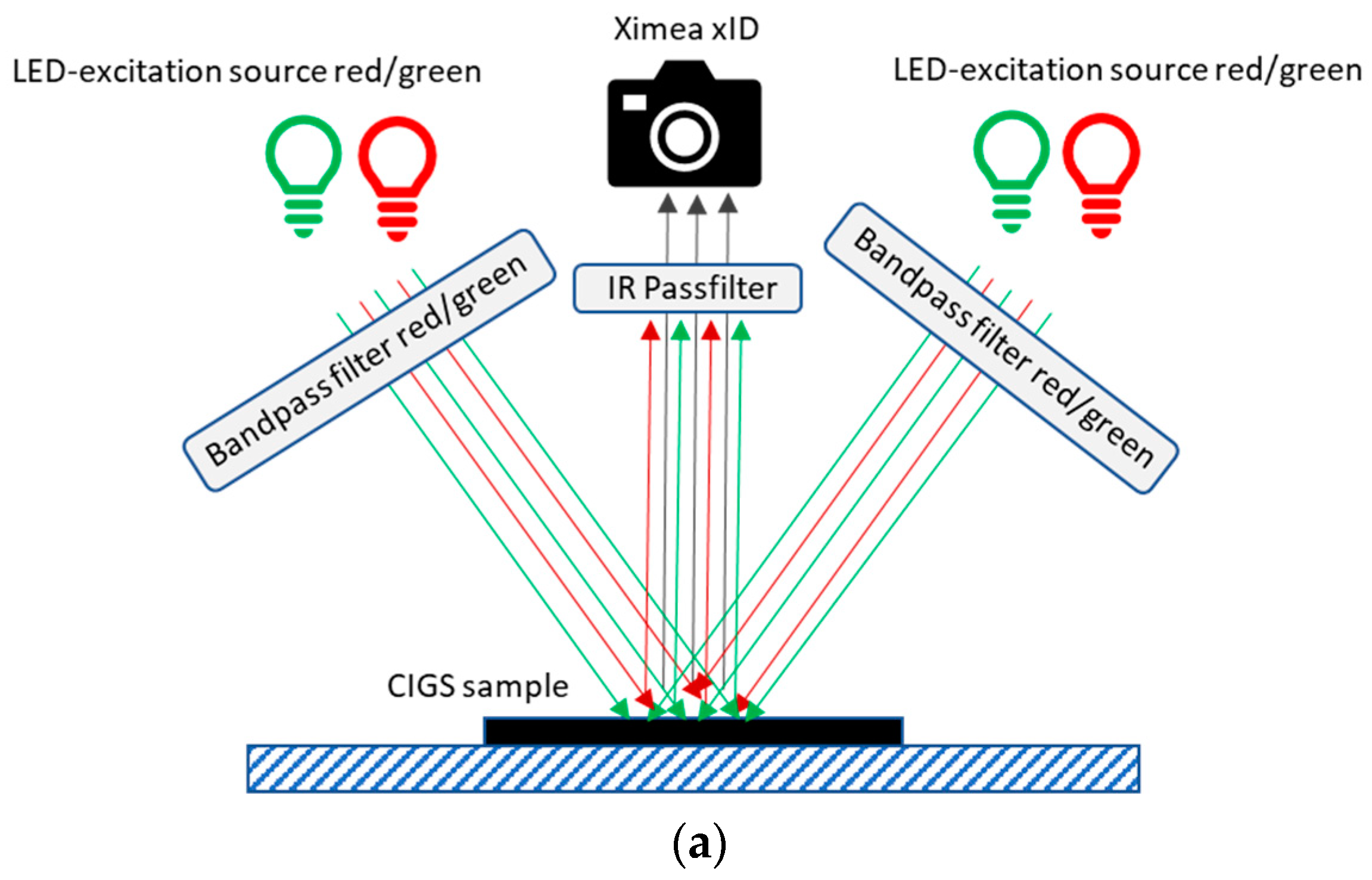
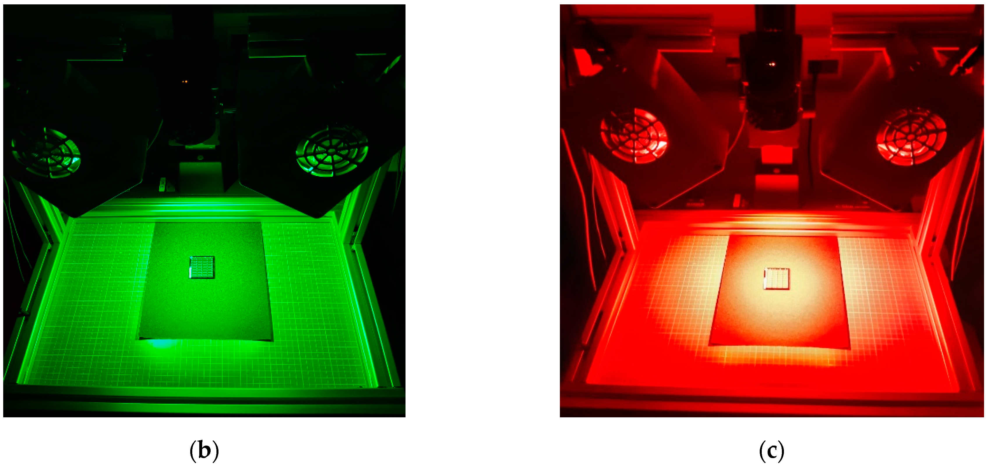
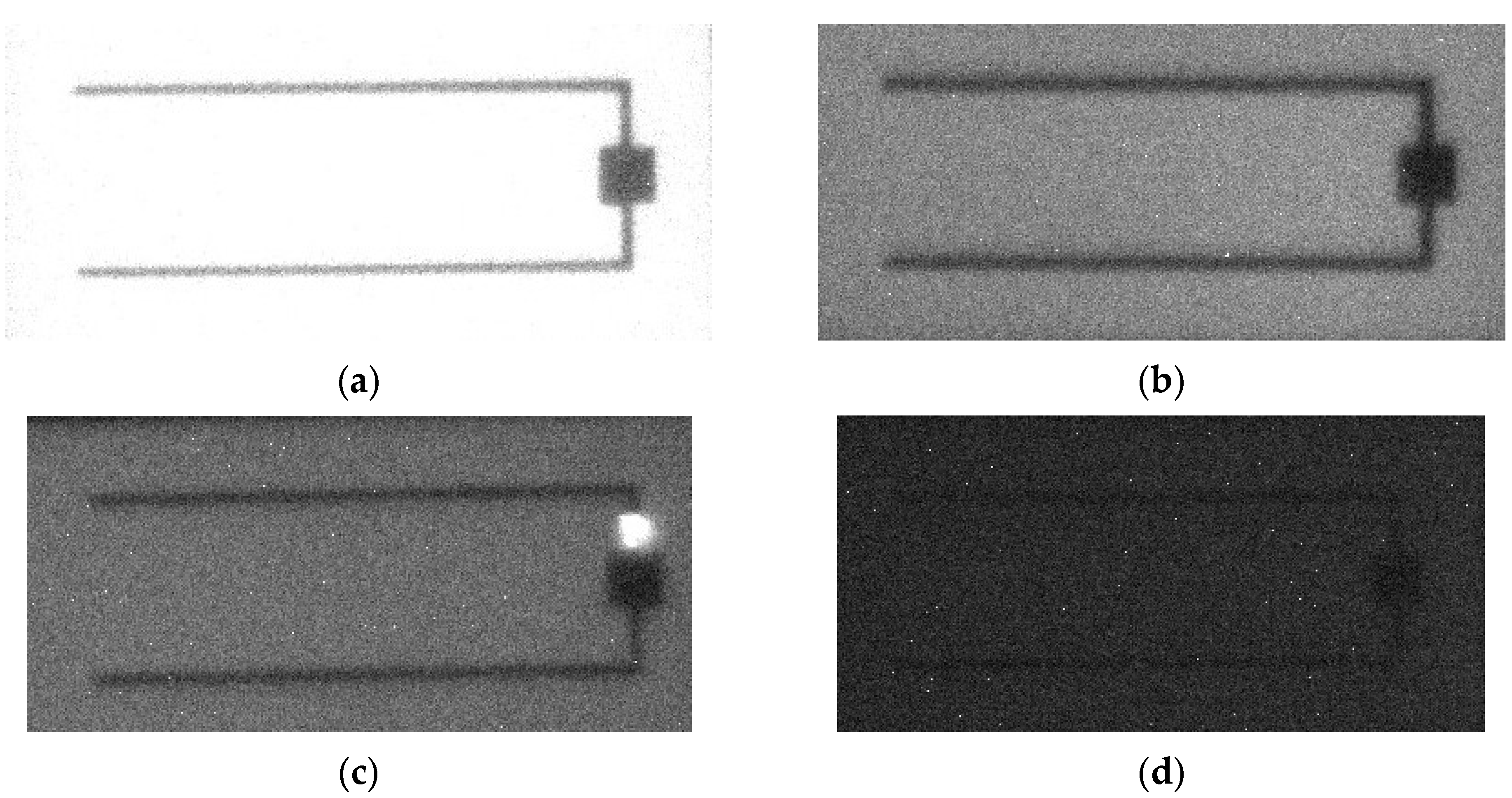
2.2. PL Image Data Acquisition

As schematically illustrated in Figure 1a, an in-line inspection demonstrator with dual-source excitation (green and red) was set up. The green excitation sources (Figure 1b) emitted at a centre wavelength of 525 nm and were operated at 2 A and 29 V, which is equivalent to a power of 58 W. This light was then bandpass-filtered by a Semrock FF01-535/150-25 filter. The red light source (Figure 1c) emitted at a centre wavelength of 625 nm, being operated at 2.5 A and 20.5 V, which equals a power of 51 W. The red excitation light source was equipped with a Semrock FF01-630/38-25 bandpass filter. To record the PL emission light, a Ximea xID (objective Qioptiq inspec.x M NIR 1.4/50 LINOS Machine Vision) camera with an IR930 VIS blocking filter was employed. The exposure time was set to 20 s at an aperture of 1.4 and a gain of 36 dB. Each sample was captured twice: one image at 0° and the other one rotated 180°. The image data were then processed in jpg data format.

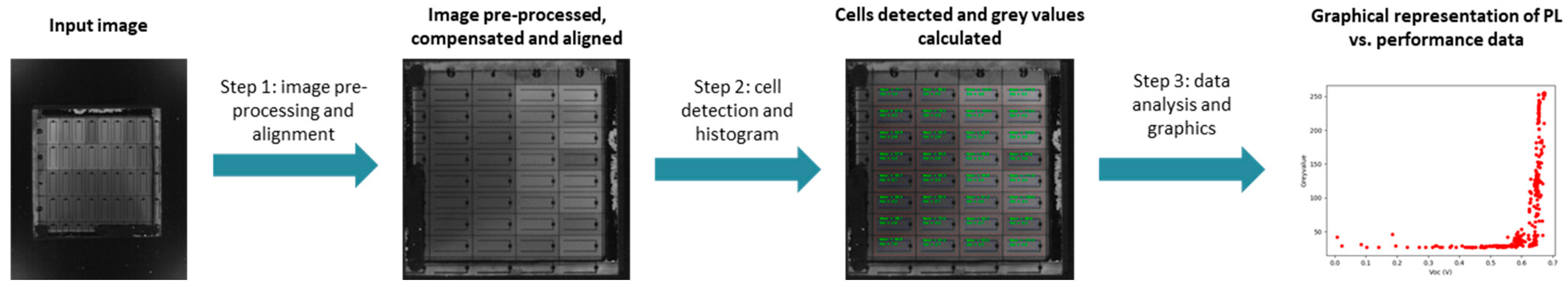
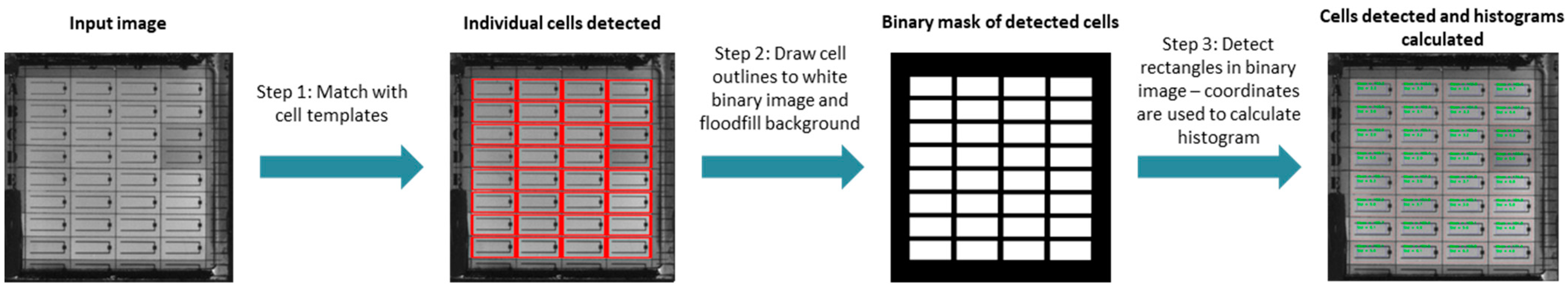
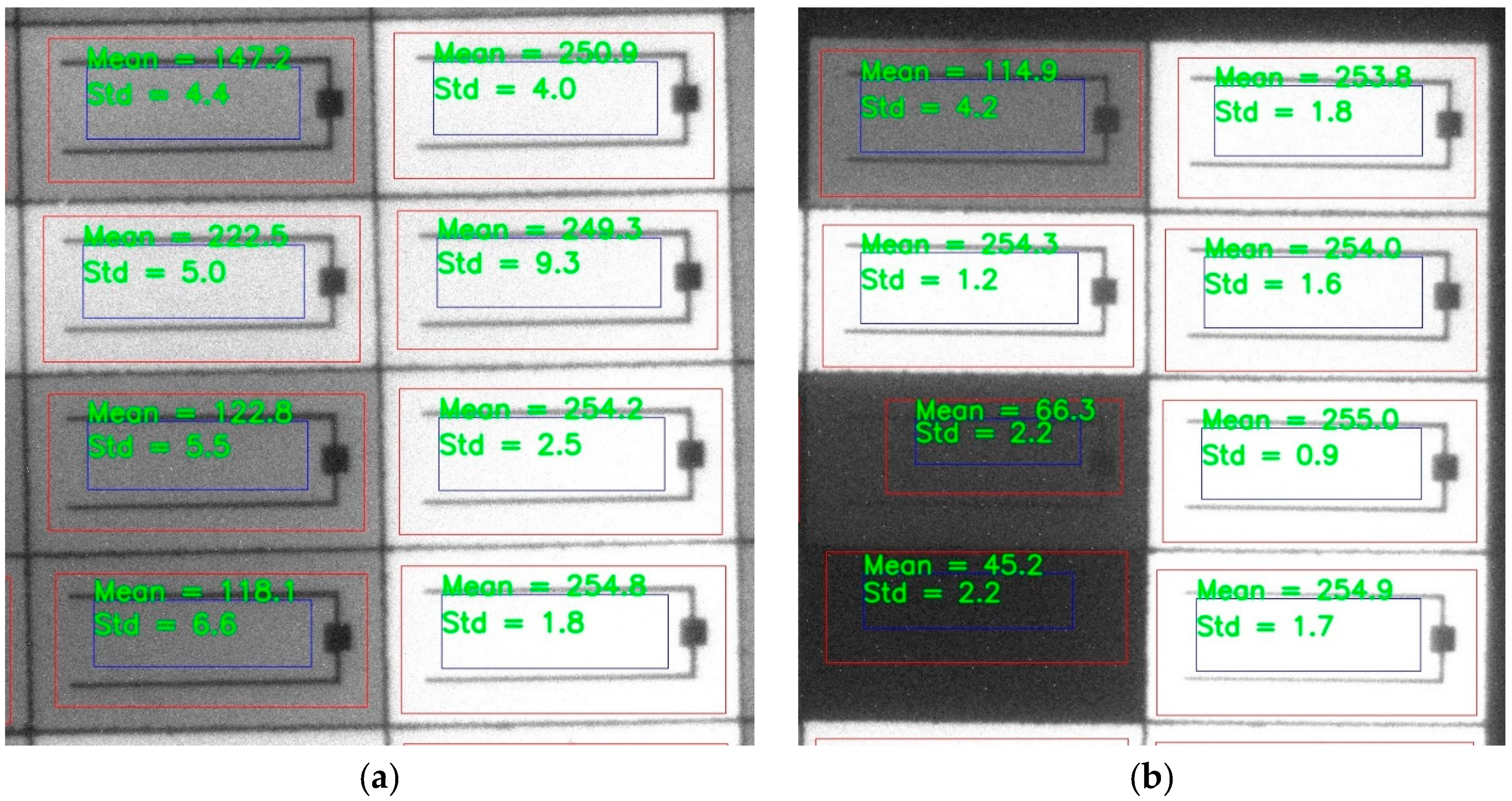
2.3. Image Processing and Data Analysis
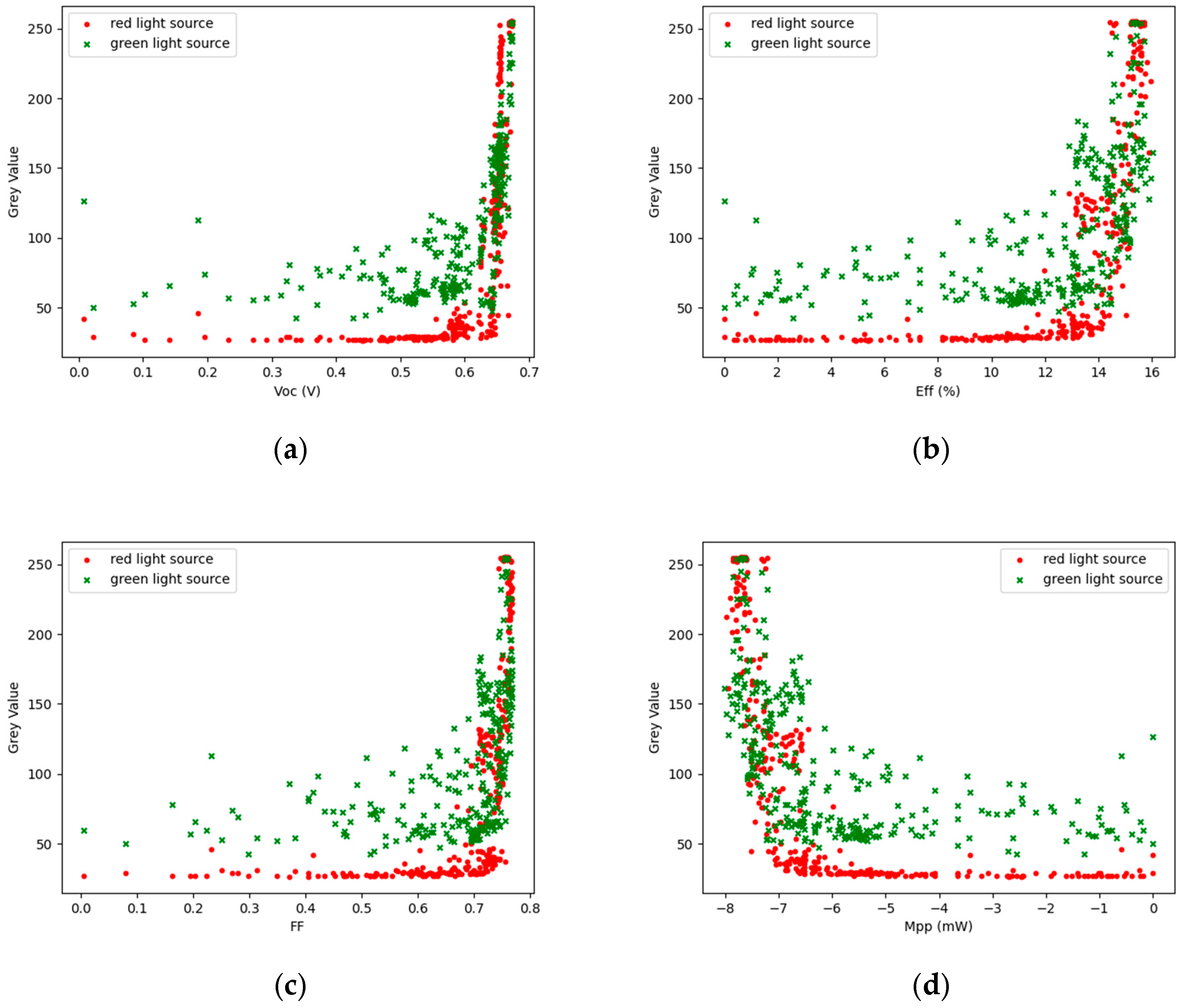
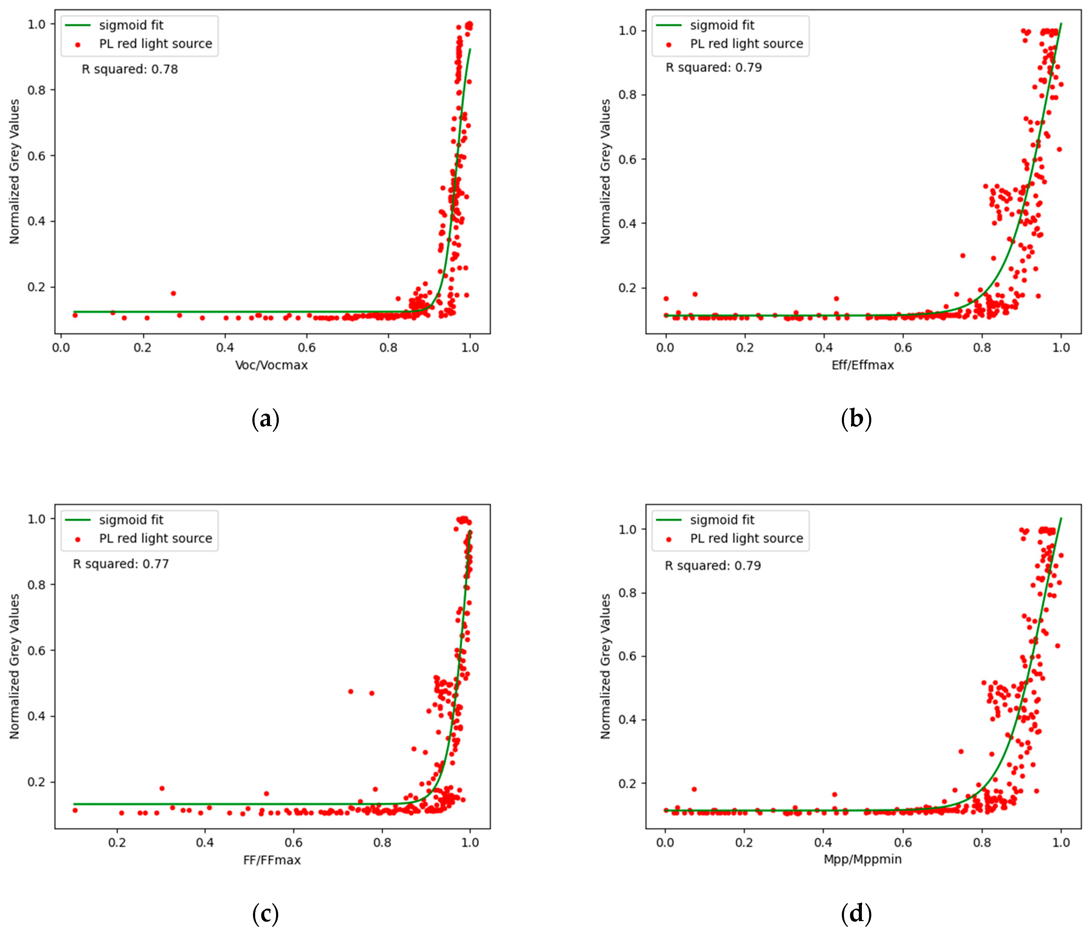
The PL images are available as 8-bit greyscale images with assigned grey values between 0 (black) and 255 (white). For automated data analysis, Python 3.8.3 including image processing libraries was used. The overall analysis process consisted of three main steps, as illustrated in Figure 2: (i) image pre-processing and alignment; (ii) cell detection and calculation of histogram; and (iii) data analysis and graphical representation of results.
Compared to the results presented in [19], a homogeneous illumination setup was implemented using a dual light source configuration and optimal alignment of the beams of the two excitation light sources. Nevertheless, image pre-processing was performed following the approach that was already presented, described, and discussed in [18]. However, as part of this work, the image pre-processing was implemented using Python, eliminating the need for manual processing. In this approach, the pre-processing is performed on the two images acquired at 0° and 180° rotation. First, the images are rotated to have the same orientation; afterwards, they are cropped utilising a uint8-mask with a given threshold and the boundingRect() function from Python’s cv2 package [26]. After cropping and alignment, the compensation of shadows and reflections is performed by several image subtraction steps in the spatial domain. The two images are low-pass filtered using a 2-dimensional Gaussian convolution kernel with a filter coefficient of σ = 200, removing all high-frequency information (i.e., detailed structures and edges) from the images. Then, those low-pass filtered images are subtracted from each other to gain information about shadows and reflections, which is then again subtracted from the original images for compensating the same.
In a subsequent step, cell detection on the pre-processed images is performed following the process illustrated in Figure 3. Therefore, Python’s cv2 matchTemplate() function is employed using pre-defined templates of the cells to be detected. In the presented approach, a small number of 7 cell templates is used, ranging from well-exposed and clearly visible cells to noisy and blurred images, as exemplarily illustrated in Figure 4. Using the matchTemplate() function, the locations of the found objects are returned. However, some of the cells are detected multiple times as they are matched to more than one template. To eliminate redundancy, a purely image-based approach is employed. The coordinates of the found rectangles are drawn to a binary image, and flood filling of the background (employing Python’s cv2 floodFill() function) creates a mask that illustrates each cell as a defined white rectangle. The coordinates of those rectangles are then again determined using Python’s cv2 boundingRect() function, providing an unambiguous location for each individual cell. In the subsequent step, the mean [0;255] as well as the standard deviations of the central areas of the individual cells are calculated using Python’s NumPy mean() and std() functions over the specified areas [27]. The results are then directly plotted in the output images.
Subsequently, the mean grey values of the individual cells under test are exported to a Microsoft Excel sheet for further analysis since in the given case, the performance data of the cells were provided as Excel data. Nonetheless, the graphical representation of the result is conducted using Python’s matplotlib scatter() as well as plot() functions, which offer multiple ways for tailored data representation [28]. For the correlation analysis, Python’s SciPy optimize package using least-squares curve fitting is employed [29].
The sensitivity or true positive rate (TPR), specificity or true negative rate (TNR), and the precision or positive predictive value (PPV) of the prediction of the cell efficiencies are then determined using the following equations:
T P R = T P T P + F N   ,
T N R = T N T N + F P   ,
P P V = T P T P + F P   ,
where TP stands for true positive, TN for true negative, FP for false positive, and FN for false negative. Those values are then illustrated in a confusion matrix.

3. Results

The sample set contained 10 CIGS samples, each consisting of 32 separate cells. The samples varied in composition (CGI and GGI ratios) as well as thickness.
For the given sample set, the cell detection functioned in a robust manner. Differences in the PL images of the cells being illuminated with green and red lights were visually observable, as exemplarily illustrated for one sample in Figure 5. It is visible to the unaided eye that the samples illuminated with green light appear to be more homogeneous than the cells illuminated with red light, which show higher-intensity variations.
The relationships between the most important cell performance parameters, namely the open-circuit voltage, efficiency, fill factor, and maximum power point, and the grey values obtained by means of PL imaging are illustrated in Figure 6a–d, respectively. The trend appears to be the same, yet it becomes obvious that illumination using the red light leads to a more defined curve progression.
The PL data using the red excitation light were further non-linearly fitted using a sigmoid function with the following Equation (5):
f ( x ) = c 1 + e k · ( x x 0 ) + f 0
where f(x) corresponds to the PL grey values and the argument x to the corresponding cell performance parameters. The parameters k, c, x0, and f0 were calculated for the individual cell performance parameters by means of least-squares curve fitting. As a measure for the fit, R2 values were calculated for each model, as illustrated in Figure 7. The resulting R2 values between 0.77 and 0.79 indicate a decent fit of the selected sigmoid function to the experimental data. The parameter f0 can be interpreted as background illumination and thermal noise with values of f0 = {0.1218; 0.1221; 0.1231; 0.1313} for the normalised representation corresponding to background grey values of g0 = {31; 31; 31; 33} for MPP, efficiency, VOC, and FF, respectively.
Table 1 shows a confusion matrix for the prediction of the cell efficiency based on PL imaging using a red light source. Therefore, it was specified that cells with an efficiency of at least 12% should be accepted, while for the PL imaging, a mean cell grey value larger than the background illumination of f0 = 31 was set as the acceptance criterion. According to Equation (2) and based on the results presented in Table 1, the sensitivity of the proposed approach is TPR = 0.94. Furthermore, the specificity is equal to TNR = 0.934 (Equation (3)) at a precision of PPV = 0.959 (Equation (4)).

4. Discussion

The PL setup consists of two green and two red excitation light sources and an industrial CCD camera for the detection of the PL signal. The emitter and the detector are equipped with optical filters to extract the spectral region of interest. The green excitation light source was selected as it can be easily filtered from the PL signal using optical filters. However, the band gap of the CdS buffer layer is in the range of 2.4 eV [30], corresponding to a wavelength of 516 nm, which leads to superimposition of the PL signal originating from the CIGS layer in the case of the green excitation light. This superimposition becomes visually observable as not only the active cells but also the surrounding areas of the samples show a fluorescent background. In addition, the influence of the CdS fluorescence leads to a high deviation when correlating the performance data with the PL imaging, as illustrated in Figure 6, especially for low-quality cells. On the other hand, this artifact could be exploited to gain information about the quality, thickness, and condition of the CdS layer itself. Those relationships will be studied as part of future work.
In contrast to that, the PL images using red excitation light led to a more defined curve progression. The data were then non-linearly fitted using a sigmoid function and least-squares minimisation, which resulted in R2 values between 0.77 and 0.79 for the experimental performance data. In contrast to previously presented results [19], this enables real quantitative assessment of the cell performance. In the given case, the samples were stored and transported between the different analysis steps (determination of performance parameters and PL imaging), which might have led to degradation of the individual cells, thus reducing the quality of the correlation. If implemented in an industrial in-line quality control system, the response time would be drastically reduced and hence the accuracy of the analysis is expected to rise further.
In general, PL imaging alone cannot give an indication of the origin of reduced PL signals, which could have material- and processing-related reasons, such as a reduced minority carrier lifetime or shunting due to laser scribing and cell contacting in later processing steps. That being said, PL imaging can be highly beneficial already at an early production step to identify and eliminate low-quality cells without the need for electrical contacts. On the other hand, cell shunting can also occur just before the modules are finalised. Consequently, implementation of PL imaging at more than one processing step as well as a combination with other in-line quality control methods, such as Raman spectroscopy, might be reasonable.
For the automated data analysis, Python was used as it is a universal, high-level programming language offering numerous advantages over other programming languages, such as a legible, concise programming style. In addition, it has an open, community-based development model supported by the non-profit Python Software Foundation [20]. The image processing approach that is presented in this work is quite straightforward, and the cell detection worked robustly even though only a small number of template images were employed. For an in-line quality control system on an industrial level, however, deep learning-based cell detection can be considered a more convenient approach. There are deep learning libraries implemented in Python such as Keras [31], which offers a uniform interface for various Python backends, such as TensorFlow, Microsoft Cognitive Toolkit (formerly CNTK), and Theano. However, due to the restricted size of the sample set, this would have gone beyond the scope of the present work.
As part of the present work, image pre-processing, cell detection, and analysis were conducted in the spatial domain, which offers easy and intuitive implementation. Some of the processing steps, such as low-pass filtering for noise reduction, could also be performed in the frequency domain; however, for most practical application tasks, Fourier-based image processing does not necessarily lead to improved results [32].
The PL images were processed in jpg data format as it is a highly versatile format that requires little memory and hence enables fast and easy processing, which is a key requirement for efficient in-line process monitoring. Speaking of processing speed, the presented PL demonstrator is comparatively slow in the given setup, as a long exposure time of 20 s is required for the acquisition of a high-quality PL image. The use of a larger number of light sources, allowing for an optimised and more homogeneous illumination, would not only result in enhancing the PL signal, and thus reducing the image acquisition time, but also in reducing the influence of shadows, reflections, and background irradiations. Furthermore, a reduced exposure time would significantly increase the compatibility of PL imaging with in-line quality control processes in the industrial mass production of CIGS solar cells.

5. Conclusions

Using a red excitation light source, PL imaging allows for qualitative as well as quantitative assessment of cell performance already at an early production step as no electrical contacts are required. For image processing, Python offers multiple powerful and easily implementable computing tools. Apart from automatised analysis methods, PL imaging provides intuitive results due to the visual representation. As a consequence, low-quality cells and batches can be identified at an early production step, which significantly reduces the response time during production, thus saving waste products, time, and costs.
For the implementation of PL imaging as an industrial in-line inspection tool for CIGS solar cells, the setup could be improved using a larger number of light sources, which would consequently reduce the exposure time and the noise level. As part of this work, a straightforward object matching approach for cell detection was employed as only a small number of samples was available. Although the presented approach functions in a robust manner, for future industrial application, deep learning could be a powerful tool to improve the quality of cell detection as well as creating predictive models for cell performance parameters.

Author Contributions

Conceptualisation, J.Z. and W.M.; methodology, J.Z. and W.M.; software, J.Z.; validation, P.J.B. and M.S.; formal analysis, P.J.B. and M.S.; writing—original draft preparation, J.Z.; writing—review and editing, W.M., P.J.B., M.S., and M.D.B.; supervision, M.D.B.; project administration, M.D.B. All authors have read and agreed to the published version of the manuscript.

Funding

The OLEDSOLAR project has received funding from the European Union’s Horizon 2020 research and innovation programme under grant agreement no. 820789.

Institutional Review Board Statement

Not applicable.

Informed Consent Statement

Not applicable.

Data Availability Statement

Not applicable.

Conflicts of Interest

The authors declare no conflict of interest.

References

  1. European Commission. Energy and the Green Deal. Available online: https://ec.europa.eu/info/strategy/priorities-2019-2024/european-green-deal/energy-and-green-deal_en (accessed on 18 October 2021).
  2. Allied Market Research. Thin Film Solar Cell Market by Type (Cadmium Telluride, Copper Indium Gallium Diselenide, and Amorphous Thin-film Silicon), End User (Residential, Commercial, and Utility), and Installation (On-Grid and Off-Grid): Global Opportunity Analysis and Industry. Available online: https://www.alliedmarketresearch.com/thin-film-solar-cell-market (accessed on 18 October 2021).
  3. Ramanujam, J.; Singh, U.P. Copper indium gallium selenide basedsolar cells—A review. Energy Environ. Sci. 2017, 10, 1306–1319. [Google Scholar] [CrossRef]
  4. Global Market Insights. Solar Cells Market Size by Technology, December 2016. Available online: https://www.gminsights.com/industry-analysis/solar-cells-market (accessed on 21 August 2020).
  5. Tang, W.; Li, X.; Lin, C.; Chen, C.; Xu, C. Production of CIGS solar cell with an appropriate atomic ratio using magnetron sputtering. Jpn. J. Appl. Phys. 2020, 59, 086502. [Google Scholar] [CrossRef]
  6. Mufti, N.; Amrillah, T.; Taufiq, A.; Sunaryono; Aripriharta; Diantoro, M.; Zulhadjri; Nur, H. Review of CIGS-based solar cells manufacturing by structural engineering. Sol. Energy 2020, 207, 1146–1157. [Google Scholar] [CrossRef]
  7. Dhimish, M.; Holmes, V. Solar cells micro crack detection technique using state-of-the-art electroluminescence imaging. J. Sci. Adv. Mater. Devices 2019, 4, 499–508. [Google Scholar] [CrossRef]
  8. Ruggeri, E.; van Aken, B.B.; Olindo, I.; Zeman, M. Electroluminescence and dark lock-in thermography for the quality assessment of metal-wrap-through solar devices. IEEE J. Photovolt. 2018, 8, 1174–1182. [Google Scholar] [CrossRef] [Green Version]
  9. Nos, O.; Favre, W.; Jay, F.; Ozanne, F.; Valla, A.; Alvarez, J.; Munoz, D.; Ribeyron, P.J. Quality control method based on photoluminescence imaging for the performance prediction of c-Si/a-Si:H heterojunction solar cells in industrial production lines. Sol. Energy Mater. Sol. Cells 2016, 144, 210–220. [Google Scholar] [CrossRef]
  10. Breitenstein, O. Local efficiency analysis of solar cells based on lock-in thermography. Sol. Energy Mater. Sol. Cells 2012, 107, 381–389. [Google Scholar] [CrossRef]
  11. Isenberg, J.; Riepe, S.; Glunz, S.W.; Warta, W. Carrier density imaging (CDI): A spatially resolved lifetime measurement suitable for in-line process-control. In Proceedings of the Conference Record of the Twenty-Ninth IEEE Photovoltaic Specialists Conference, New Orleans, LA, USA, 19–24 May 2002. [Google Scholar]
  12. Ziska, C.; Ossig, C.; Pyrlik, N.; Carron, R.; Avancini, E.; Fevola, G.; Kolditz, A.; Siebels, J.; Kipp, T.; Cai, Z.; et al. Quantifying the elemental distribution in solar cells from X-ray fluorescence measurements with multiple detector modules. In Proceedings of the 47th IEEE Photovoltaic Specialists Conference (PVSC), Calgary, AB, Canada, 15–21 August 2020. [Google Scholar]
  13. Stuckelberger, M.E.; Nietzold, T.; West, B.; Fashchi, R.; Poplavskyy, D.; Bailey, J.; Lai, B.; Maser, J.M.; Bertoni, M. Defect activation and annihilation in CIGS solar cells: An operando x-ray microscopy study. J. Phys. Energy 2020, 2, 025001. [Google Scholar] [CrossRef]
  14. Parravicini, J.; Acciarri, M.; Murabito, M.; Le Donne, A.; Gasparotto, A.; Binetti, S. In-depth photoluminescence spectra of pure CIGS thin films. Appl. Opt. 2018, 57, 1849–1856. [Google Scholar] [CrossRef] [PubMed]
  15. Repins, I.; Contreras, M.; Romero, M.; Yan, Y.; Metzger, W.; Li, J.; Johnston, S.; Egaas, B.; DeHart, C.; Scharf, J.; et al. Characterization of 19.9%-efficient CIGS absorbers. In Proceedings of the 33rd IEEE Photovoltaic Specialists Conference, San Diego, CA, USA, 11–16 May 2008. [Google Scholar]
  16. Lin, L.; Ravindra, N.M. Temperature dependence of CIGS and perovskite solar cell performance: An overview. SN Appl. Sci. 2020, 2, 1361. [Google Scholar] [CrossRef]
  17. Lawerenz, A.; Lauer, K.; Blech, M.; Laades, A.; Zentgraf, M. Photoluminescence lifetime imaging using LED arrays as excitation source. In Proceedings of the 25th European Photovoltaic Solar Energy Conference and Exhibition/5th World Conference on Photovoltaic Energy Conversio, Valencia, Spain, 6–10 September 2010; pp. 2486–2489. [Google Scholar]
  18. De Biasio, M.; Zikulnig, J.; Mühleisen, W.; Kraft, M.; Simor, M.; Bolt, P.J. Inline inspection of CIGS solar cells by means of Raman spectroscopy and photoluminescence imaging. In Next-Generation Spectroscopic Technologies XIV; International Society for Optics and Photonics: Bellingham, WA, USA, 2021; Volume 11725. [Google Scholar]
  19. Zikulnig, J.; Harms, K.; Mühleisen, W.; Neumaier, L.; Bolt, P.J.; Simor, M.; de Biasio, M. Raman spectroscopy as a possible in-line inspection tool for cigs solar cells in comparison with photoluminescence measurements. In Proceedings of the 37th European Photovoltaic Solar Energy Conference and Exhibition, Lisbon, Portugal, 7–11 September 2020. [Google Scholar]
  20. Python Software Foundation. Python Software Foundation. Available online: https://www.python.org/psf/ (accessed on 21 October 2021).
  21. Statista. Most Used Programming Languages among Developers Worldwide, as of 2021. Available online: https://www.statista.com/statistics/793628/worldwide-developer-survey-most-used-languages/ (accessed on 21 October 2021).
  22. Annala, L.; Eskelinen, M.; Hämäläinen, J.; Riihinen, A.; Pölönen, I. Practical approach for hyperspectral image processing in Python. Int. Arch. Photogramm. Remote Sens. Spat. Inf. Sci. 2018, 42, 45–52. [Google Scholar] [CrossRef] [Green Version]
  23. Gouillart, E.; Nunez-Iglesias, J.; van der Walt, S. Analyzing microtomography data with Python and the scikit-image library. Adv. Struct. Chem. Imaging 2016, 2, 18. [Google Scholar] [CrossRef] [PubMed] [Green Version]
  24. Widodo, C.E.; Adi, K.; Gernowo, R. Medical image processing using python and open cv. J. Phys. Conf. Ser. 2020, 1524, 012003. [Google Scholar] [CrossRef]
  25. Deitsch, S.; Buerhop-Lutz, C.; Sovetkin, E.; Steland, A.; Maier, A.; Gallwitz, F.; Riess, C. Segmentation of photovoltaic module cells in uncalibrated electroluminescence images. Mach. Vis. Appl. 2021, 32, 84. [Google Scholar] [CrossRef]
  26. Python Software Foundation. Opencv-Python 4.5.4.58. Available online: https://pypi.org/project/opencv-python/ (accessed on 27 October 2021).
  27. NumPy. All Rights Reserved. NumPy. Available online: https://numpy.org/ (accessed on 27 October 2021).
  28. Hunter, J.D. Matplotlib: A 2D graphics environment. Comput. Sci. Eng. 2007, 9, 90–95. [Google Scholar] [CrossRef]
  29. SciPy. SciPy—Fundamental Algorithms for Scientific Computing in Python. 2021. Available online: https://scipy.org/ (accessed on 5 November 2021).
  30. Ariza-Calderon, H.; Lozada-Morales, R.; Zelaya-Angel, O.; Mendoza-Alvarez, J.G.; Banos, L. Photoluminescence measurements in the phase transition region for CdS thin films. J. Vac. Sci. Technol. 1996, 14, 2480. [Google Scholar] [CrossRef]
  31. Keras. Keras. Available online: https://keras.io/ (accessed on 5 November 2021).
  32. Usman, B.; Ayuba, S. Practical Digital Image Enhancements using Spatial and Frequency Domains Techniques. Int. Res. J. Comput. Sci. 2015, 2, 27–32. [Google Scholar]
Figure 1. (a) Schematic illustration of the PL imaging setup using dual light source configuration; (b) illumination of CIGS sample using a green light source; (c) illumination of CIGS sample using a red light source.
Solar 02 00001 g001aSolar 02 00001 g001b
Figure 2. Overview of the image processing flow consisting of three major steps: image pre-processing and alignment; cell detection and calculation of histogram; and data analysis and graphical representation of results.
Solar 02 00001 g002
Figure 3. Cell detection process flow consisting of three major steps: match the pre-processed input image with the cell templates; draw the coordinates of the found cells to a binary image and flood fill the background; and detect rectangles in the binary image and use those coordinates to calculate histogram data of cells in the input image.
Solar 02 00001 g003
Figure 4. Examples of cell templates used for cell detection: (a) bright, overexposed; (b) medium brightness; (c) medium brightness with optical disruption of the contacts; (d) dark with salt and pepper noise.
Solar 02 00001 g004
Figure 5. Example of PL images of the same cell sample after pre-processing and cell detection using (a) green and (b) red excitation lights.
Solar 02 00001 g005
Figure 6. Relationship between measured grey values and the most relevant cell performance parameters, namely (a) open-circuit voltage (VOC), (b) efficiency (Eff), (c) fill factor (FF), and (d) maximum power point (MPP), for green and red excitation illumination.
Solar 02 00001 g006
Figure 7. Non-linear normalised fitting of grey values (red excitation) and (a) open-circuit voltage (VOC), (b) cell efficiency, (c) fill factor (FF), and (d) maximum power point (MPP).
Solar 02 00001 g007
Table 1. Confusion matrix for the prediction of the cell efficiency based on PL imaging using red light source (acceptance criteria: actual: 12% efficiency; predicted: grey value > 31).
Predicted Positive
(Grey Value > 31)
Predicted Negative
(Grey Value ≤ 31)
Sum
Actual Positive
(Eff > 12%)
18612198
Actual Negative
(Eff ≤ 12%)
8114122
Sum194126320
Publisher’s Note: MDPI stays neutral with regard to jurisdictional claims in published maps and institutional affiliations.

