Article

Financial Time Series Modelling Using Fractal Interpolation Functions

by
Polychronis Manousopoulos
1,*,
Vasileios Drakopoulos
2 and
Efstathios Polyzos
3
1
Bank of Greece, 21 Eleftherios Venizelos Avenue, 10250 Athens, Greece
2
Department of Computer Science and Biomedical Informatics, University of Thessaly, 35131 Lamia, Greece
3
College of Business, Zayed University, Abu Dhabi P.O. Box 144534, United Arab Emirates
*
Author to whom correspondence should be addressed.
AppliedMath 2023, 3(3), 510-524; https://doi.org/10.3390/appliedmath3030027
Submission received: 12 May 2023 / Revised: 23 June 2023 / Accepted: 27 June 2023 / Published: 29 June 2023

Abstract

:
Time series of financial data are both frequent and important in everyday practice. Numerous applications are based, for example, on time series of asset prices or market indices. In this article, the application of fractal interpolation functions in modelling financial time series is examined. Our motivation stems from the fact that financial time series often present fluctuations or abrupt changes which the fractal interpolants can inherently model. The results indicate that the use of fractal interpolation in financial applications is promising.

1. Introduction

Time series of financial data such as asset prices or market indices occur frequently in everyday practice. The modelling, analysis and prediction of financial time series is an important tool in decision making for institutions or investors; see, for example [1], and [2]. It is not uncommon that financial time series are not smooth but exhibit significant fluctuations, because of reflecting a financial crisis or market turbulence. This provides an adequate motive of examining methods that inherently allow fluctuations when modelling such time series.
Fractal interpolation, as defined in [3], provides a framework for interpolating irregular, non-smooth sets of data, which possibly exhibit self-similarity and details at different scales. While traditional interpolation techniques are based on smooth functions such as polynomials and generate smooth interpolants, fractal interpolation is founded on the theory of iterated function systems (IFSs, see [4]) and is able to model irregular sets of data such as projections of physical objects, e.g., coastlines, or experimental data of non-integral dimension. See [5,6], for example, for such successful applications of fractal interpolation.
Financial time series are typically modelled using autoregressive integrated moving average (ARIMA) or generalised autoregressive conditional heteroskedasticity (GARCH) models; see e.g., [7,8,9,10,11,12]. These models take into account the autoregressive properties of such data and are thus commonly used in the existing literature to model returns/growth rates (ARIMA) or volatility (GARCH). In the last few years, there is an emerging trend using machine learning or deep learning approaches, such as Support Vector Machines (SVM), Long Short-Term Memory (LSTM) or other neural networks ([13,14,15,16]). Such approaches can provide greater predicting accuracy but are often prone to overfitting, thus resulting in data-specific findings ([17]). Furthermore, machine and deep learning approaches are also criticized for lack of interpretability ([18]), as these models are only able to supply numerical forecasts without providing interpretable results (such as coefficients or standard errors) that would improve our theoretical understanding of the underlying mechanism at work; a new trend in Artificial Intelligence, termed eXplainable AI (XAI), aims to address this issue ([19,20]).
In this article, we examine the application of fractal interpolation to the modelling of financial time series. As previously mentioned, fractal interpolation functions are a suitable candidate for this application. The use of fractal techniques in the analysis of financial data is seen occasionally in the literature, see e.g., [21,22,23,24,25,26,27,28,29,30]. However, in most cases IFS-based fractal interpolation is not used; in the previous references the sole exception is [25], where a simple example of comparing self-affine fractal interpolation to linear interpolation of the values of a company’s assets is presented. Here we perform in-sample and out-of-sample tests on a variety of sets of data (bitcoin prices, S&P 500, U.S. GDP) which possess different characteristics, such as time span and smoothness. The results indicate that fractal interpolation functions are indeed successful in in this area, even when a sparse selection of interpolation points is made.
The article is structured as follows. Section 2 presents the elementary concept of both iterated functions system and the fractal interpolation function. Section 3 presents the results of modelling financial time series with fractal interpolation functions. Finally, Section 4 summarises our conclusions and indicates areas of future work.

2. Fractal Interpolation

Fractal interpolation, as defined in [3], is based on the theory of iterated function systems. Here we present the basic concepts; for more details see [4].

2.1. Iterated Function Systems

Let X , ρ be a complete metric space, for instance R n , · . A function f : X X is called a Lipschitz function, if there exists k R such that ρ f x , f ( y ) k ρ ( x , y ) , for all x , y X ; by definition k 0 . If k < 1 , then f is called a contraction with contractivity factor  k . Let H ( X ) denote the set of nonempty, compact subsets of X . The metric space H X , h , where h is an appropriate metric, e.g., the Hausdorff metric, is often called the “space of fractals”. Note that not every member of H X is necessarily a fractal.
An iterated function system (or IFS for short) consists of a complete metric space X , ρ together with a finite set of continuous mappings w n : X X , n = 1 , 2 , , N . An IFS is denoted as X ; w n , n = 1 , 2 , , N . If all mappings w n are contractions with contractivity factors s n , n = 1 , 2 , , N , then the IFS is called hyperbolic with contractivity factor s = max n = 1 , 2 , , N s n . Let W : H ( X ) H X be the mapping defined as W B = n = 1 N w n B , where B H X and w n B = w n b , b B . Each hyperbolic IFS has a unique attractor which is the set A H X , with A = W A = lim n W n ( B ) for every B H X , where W n denotes the n -fold composition W W W . Therefore the attractor A is the unique fixed point of W and every set B H X converges to it under successive applications of W . The term attractor stems from this property, which also provides the basis for the computational construction of an IFS attractor. Specifically, the deterministic iteration algorithm or the random iteration algorithm (see e.g., [4]) can be used for constructing an IFS attractor.

2.2. Self-Affine Fractal Interpolation Functions

Let Δ 1 be a partition of the real compact interval I = [ a , b ] , i.e., Δ 1 = u 0 , u 1 , , u M where a = u 0 < u 1 < < u M = b . Let the set of data points be represented as P = u m , v m I × R , m = 0 , 1 , , M . Let Δ 2 be another partition of I = [ a , b ] , i.e., Δ 2 = x 0 , x 1 , , x N where a = x 0 < x 1 < < x N = b , such that Δ 1 is a refinement of Δ 2 . Let the set of interpolation points be represented as Q = x i , y i I × R , i = 0 , 1 , , N M , while it is a subset of the data points, i.e., Q P . The subintervals of Δ 2   x i , x i + 1 , i = 0 , 1 , , N 1 , are called interpolation intervals; the abscissas x i of the interpolation points may be equidistant or not. The set of data points within the nth interpolation interval I n = x n 1 , x n , n = 1 , 2 , , N , is denoted as P n = u m , v m : x n 1 u m x n ; obviously, it is P = n = 1 N P n .
An affine transformation is defined as the composition of a linear transformation and a translation. Let R 2 ; w n , n = 1 , 2 , , N be an iterated function system with affine transformations
w n x y = a n 0 c n s n x y + d n e n
satisfying the constraints
w n x 0 y 0 = x n 1 y n 1   and   w n x N y N = x n y n
for every n = 1 , 2 , , N . In other words, I is mapped by each affine transformation w n to its corresponding interpolation interval. Solving the above equations leads to
a n = x n x n 1 x N x 0 ,   d n = x N x n 1 x 0 x n x N x 0
c n = y n y n 1 x N x 0 s n y N y 0 x N x 0 ,   e n = x N y n 1 x 0 y n x N x 0 s n x N y 0 x 0 y N x N x 0
i.e., the real parameters a n , c n , d n , e n are uniquely determined by the interpolation points, while the real parameters s n are free parameters of the transformations such that s n < 1 , n = 1 , 2 , , N . This constraint is necessary to guarantee that the IFS is hyperbolic with respect to an appropriate metric. The transformations w n are shear transformations, i.e., they map line segments parallel to the y -axis to line segments also parallel to the y -axis contracted by a factor s n . For this reason, the parameters s n are called vertical scaling factors or contractivity factors of the transformations w n .
The attractor of the afore-mentioned IFS, i.e., the unique set G = n = 1 N w n G , is the graph of a continuous function f : x 0 , x N R that passes through all interpolation points x i , y i , i = 0 , 1 , , N . This function is called fractal interpolation function, or FIF for short, corresponding to these points. It is a self-affine function since each affine transformation w n maps the entire graph of the function to its section within the corresponding interpolation interval.
An example of a fractal interpolation function is presented in Figure 1, where a set of ten interpolation points and vertical scaling factors s n = 0.25 , n = 1 , 2 , , 10 are used. Note that from a simple set of few points a complicated interpolant is generated.
The remaining data points  P Q are only approximated by the fractal interpolation function, which does not necessarily pass through them. To optimise the fit of the data points for a given set of interpolation points, the vertical scaling factors, the only free parameters, must be appropriately determined. Various methods have been proposed in the literature for calculating them. Usually, the vertical scaling factors are calculated by minimising an error measure, such as the squared error between the ordinates of the original and the reconstructed points m = 0 M v m G u m 2 , where G u m is the attractor ordinate at abscissa u m , or the Hausdorff metric h P , G . For example, in [31] an analytic and a geometric method are proposed for minimising this squared error. In [32, 33] the use of bounding volumes of data points subsets is proposed, to optimise the fit between original and transformed bounding volumes instead of individual points. Other methods use different approaches instead of minimising an error measure; in [34] the target is to preserve the fractal dimension of the data points; in [35] the target is to detect self-affinity and the implied vertical scaling factors in the continuous wavelet transform of the data.
An additional example of a fractal interpolation function is depicted in Figure 2. A set of 37 data points is interpolated by a fractal interpolation function using every 3rd point as interpolation points, i.e., 13 points in total; the vertical scaling factors are calculated by the geometric algorithm of [31]. Despite of the use of approximately only 1/3 of the data points and the simple, equidistant selection of the interpolation points, the remaining data points are approximated rather well.
It is worth noting that although one could use all data points as interpolation points thus guaranteeing that the resulting fractal interpolation function passes through all of them, this is not always desirable in practice. A proper selection of interpolation points, along with optimal calculation of the vertical scaling factors, will result in satisfactory goodness of fit and a considerable compression ratio without overfitting. Note that the interpolation points should not necessarily be equidistant, but can be also selected to minimise an error measure, see e.g., [31].

2.3. Recurrent Fractal Interpolation Functions

The recurrent fractal interpolation functions are a generalization of the self-affine fractal interpolation functions of the previous section. This is achieved by allowing piecewise instead of total self-affinity. Initially, the partitions Δ 1 and Δ 2 of the interval I , the set P of data points and its subsets P n , the set Q of interpolation points and the interpolation intervals I n , are all defined as in the previous section. Additionally, each interpolation interval is associated with a pair of data points called address points. Specifically, each interpolation interval I n = x n 1 , x n , n = 1 , 2 , , N is associated with two distinct data points x n , 1 , y n , 1 , x n , 2 , y n , 2 P , i.e., x n , k , y n , k = u m k , , v m k for k = 1 , 2 and some m k 0 , 1 , , M . Each pair of address points defines the address interval  x n , 1 , x n , 2 , where x n , 1 < x n , 2 by definition. The address points are not necessarily unique among interpolation intervals, i.e., a data point may be used in more than one address interval. Moreover, every address interval should have strictly greater length than its corresponding interpolation interval, i.e., x n , 2 x n , 1 > x n x n 1 , for all n = 1 , 2 , , N . The set of data points within the nth address interval I n = x n , 1 , x n , 2 , n = 1 , 2 , , N , is denoted as A n = u m , v m : x n , 1 u m x n , 2 .
Let R 2 ; w n , n = 1 , 2 , , N be an iterated function system with affine transformations
w n = x y = a n 0 c n s n x y + d n e n
satisfying the constraints
w n x n , 1 y n , 1 = x n 1 y n 1   and   w n x n , 2 y n , 2 = x n y n
for every n = 1 , 2 , , N . In other words, each address interval is mapped to its corresponding interpolation interval. Solving these constraint equations leads to
a n = x n x n 1 x n , 2 x n , 1 ,   d n = x n , 2 x n 1 x n , 1 x n x n , 2 x n , 1
c n = y n y n 1 x n , 2 x n , 1 s n y n , 2 y n , 1 x n , 2 x n , 1 ,   e n = x n , 2 y n 1 x n , 1 y n x n , 2 x n , 1 s n x n , 2 y n , 1 x n , 1 y n , 2 x n , 2 x n , 1
i.e., the real parameters a n , c n , d n , e n are uniquely determined by the interpolation points and the address points, while the real parameters s n are free parameters of the transformations such that s n < 1 , n = 1,2 , , N . This constraint is necessary to guarantee that the resulting IFS is hyperbolic with respect to an appropriate metric. As previously, the transformations w n are shear transformations and the parameters s n are called vertical scaling factors or contractivity factors of the transformations w n .
The attractor of the aforementioned IFS, i.e., the unique set G = n = 1 N w n G , is the graph of a continuous function f : x 0 , x N R that passes through all interpolation points x i , y i , i = 0,1 , , N . This function is called recurrent fractal interpolation function (RFIF) corresponding to these points. It is a piecewise self-affine function since each affine transformation w n maps the part of the graph of the function within the corresponding address interval to its section within the corresponding interpolation interval. Note that when all address intervals are equal to the interval I , then the recurrent fractal interpolation function reduces to a fractal interpolation function of the previous section.
An example of a recurrent fractal interpolation function is presented in Figure 3, where the set of interpolation points of Figure 1 is used; the address intervals are distinct and the vertical scaling factors are s n = 0.25 , n = 1 , , 10 . Although the same vertical scaling factors as in Figure 1 have been used, the resulting interpolant is smoother. This is because each address intervals contains fewer interpolation points than the whole function, thus resulting in smaller variation within the respective interpolation interval to which it is mapped.
The remaining data points P Q are approximated by the recurrent fractal interpolation function, since it does not necessarily pass through them. In order to optimise the fit, the vertical scaling factors are calculated by methods similar to those described in the previous section for the fractal interpolation functions. These include methods that minimise an error measure, such as the analytic and geometric methods of [31], or the bounding volumes method of [32,33]. Other methods employ the use of fractal dimension ([34]) or wavelets ([35]). The remarks of previous section about the selection of the interpolation points apply here as well.
An additional example is depicted in Figure 4. The set of data points and interpolation points of Figure 2 is used, the address intervals are of variable length and the vertical scaling factors are calculated by the analytic algorithm of [31]. Note that the recurrent interpolant approximates even better the remaining data points. This is allowed by the property of partial, piecewise self-affinity, in contrast to the total self-affinity of the fractal interpolant of Figure 2.

3. Financial Time Series Modelling

In this section, we present three cases of financial time series modelling. Each case is different with respect to the extent or the characteristics of the underlying data set. Our aim is to show the suitability of fractal interpolation in a diversity of applications. There are inherent difficulties in modelling and predicting financial data series of different forms. Cryptocurrency prices exhibit significant volatility [36], stock market indices are susceptible to external shocks [37], while GDP data is affected by economic cycles which can have indeterminate duration [38]. Thus, an adaptable methodology that would permit short-term forecasts or accurate interpolation to higher frequency data could be very useful to researchers.

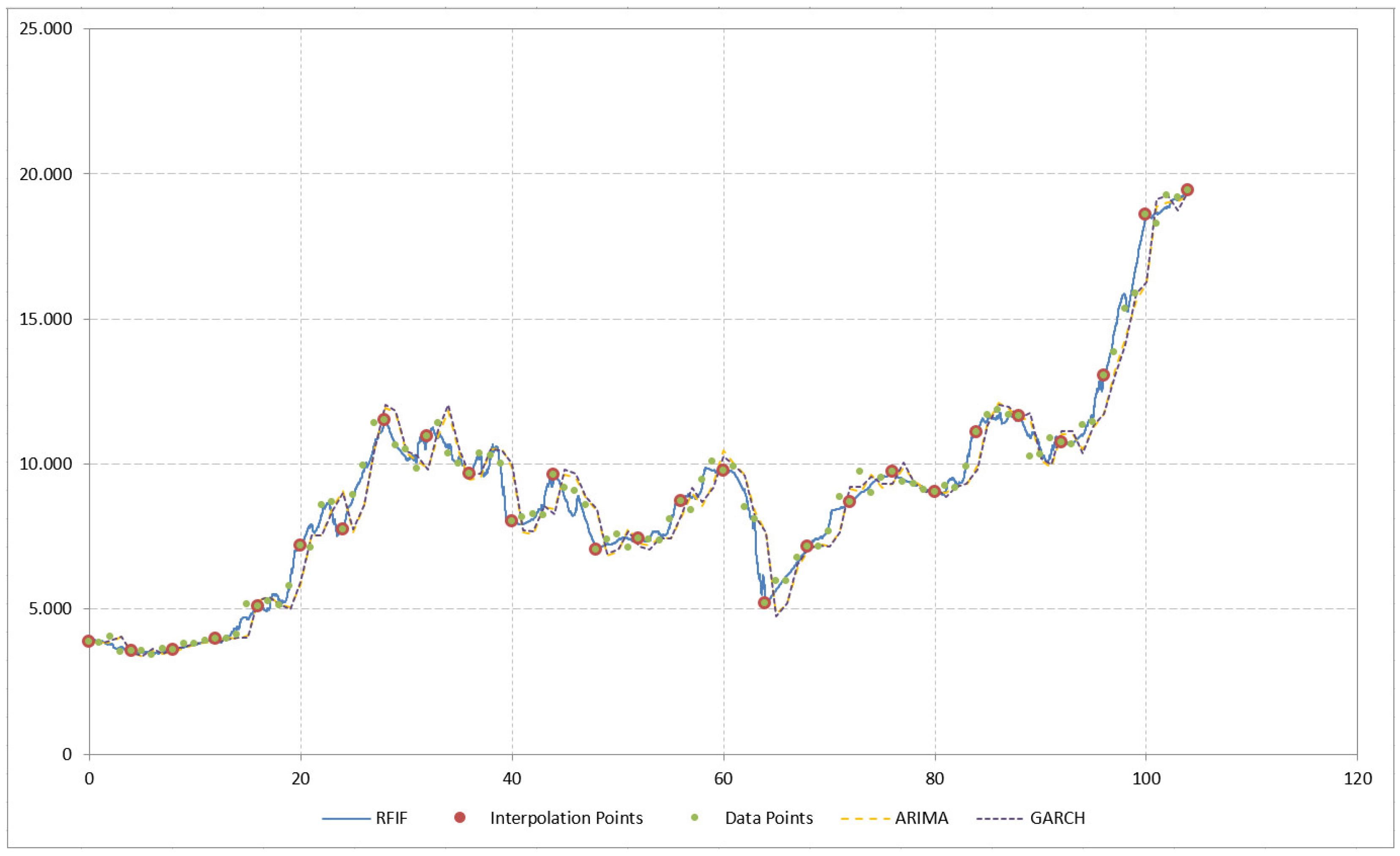
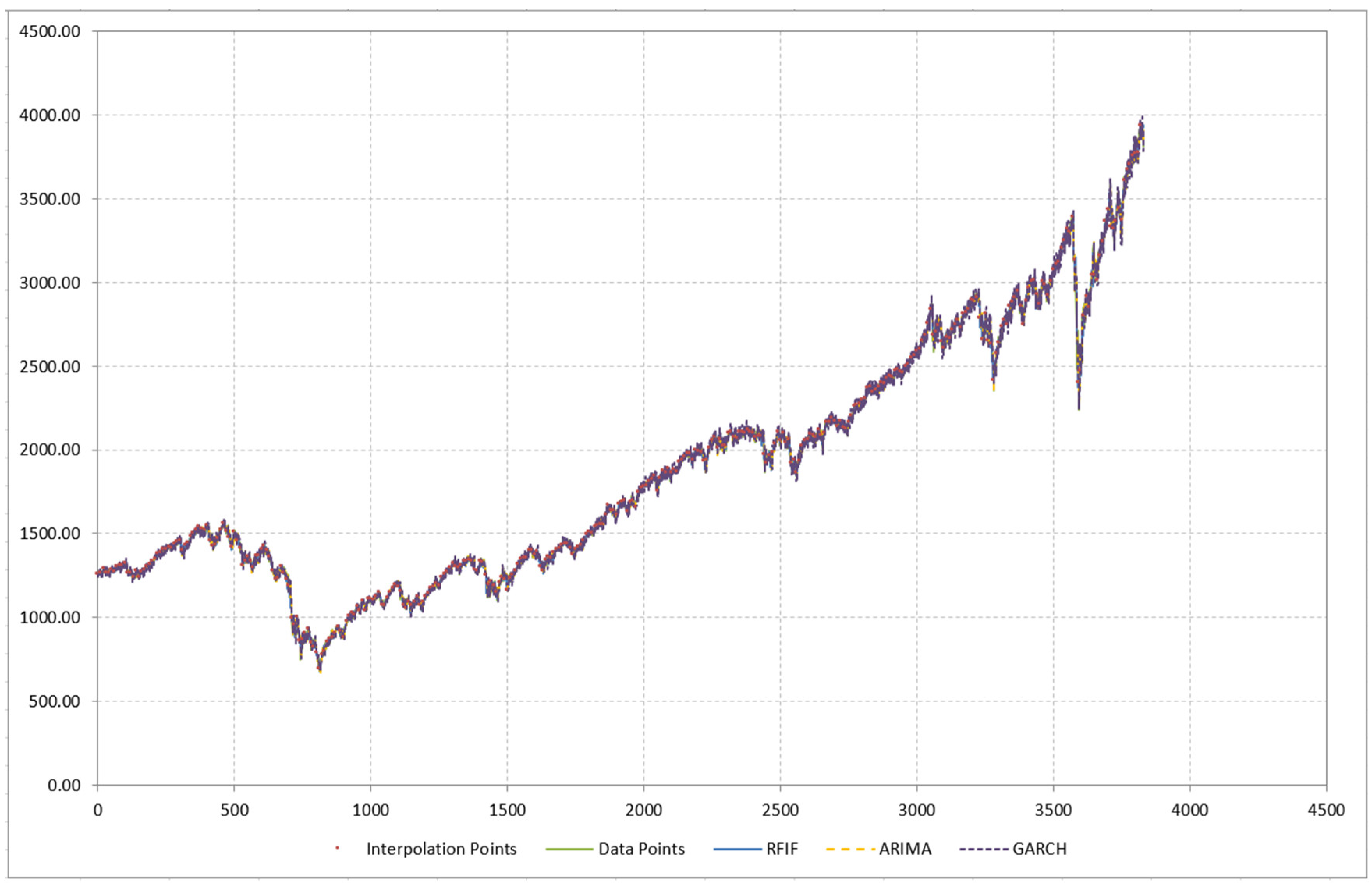
3.1. Dataset 1—Bitcoin Prices

The first set of data consists of bitcoin historical prices. Bitcoin is a decentralized digital cryptocurrency that allows direct transactions between members of a peer-to-peer network without the need of a trusted third party [39]. It emerged in 2009 and has gained widespread popularity and use since then. The data set has a two-year time span. Specifically, it consists of weekly prices from 23 December 2018 to 16 December 2020 containing a total of 105 data points (data obtained from Bloomberg Professional (accessed on 18 April 2021)). The time series has been modelled by a recurrent fractal interpolation function as depicted in Figure 5. For constructing the interpolant, every 4th data point is used as interpolation point, resulting in a total of 27 interpolation points. The address intervals have a fixed span of 25 data points; for each interpolation interval I n , the optimal address interval has been selected between possible candidates by minimising the Hausdorff distance between the original and mapped data points, i.e., A n = arg min A A ( P , l ) h P n , w n A , n = 1,2 , , N , where A ( p , l ) denotes the subsets of P spanning l consecutive data points. The vertical scaling factors are calculated using the analytic algorithm of [31]. Note that although only 1 / 4 of the data points are used, the fractal interpolant represents successfully the time series; the fluctuations of the underlying dataset are correctly captured. However, this would not be the case if a smooth interpolant, e.g., a cubic spline, was used for the same set of interpolation points.

3.2. Dataset 2—S&P 500

The second set of data consists of S&P 500 historical values. The S&P 500 is a stock market index; specifically, it is a capitalization weighted index of 500 large cap companies publicly traded in the U.S. (S&P 500, available online: https://en.wikipedia.org/wiki/S%26P_500 (accessed on 2 December 2021)). It is considered to be one of the best indicators of U.S. equities performance and it is widely followed by investors and institutions. The data set has a 15-year time span approximately. Specifically, it consists of daily values from 9 December 2005 to 1 March 2021 containing a total of 3830 data points (data obtained from Bloomberg Professional (accessed on 18 April 2021)). The time series has been modelled by a recurrent fractal interpolation function as depicted in Figure 6. For constructing the interpolant, every 10th data point is used as interpolation point, resulting in a total of 383 interpolation points. The address intervals have a fixed span of 25 data points; for each interpolation interval I n , the optimal address interval is selected between possible candidates by minimising the Hausdorff distance between the original and mapped data points, as in the first dataset. The vertical scaling factors are calculated using the analytic algorithm of [31]. Note that although only 1 / 10 of the data points are used, the fractal interpolant is able to represent accurately the time series. This is more clearly shown in Figure 7, which depicts the part of Figure 6 between the 3630th and the 3820th data points. In Figure 7, we see that the fractal interpolant closely follows the data points despite the considerable sparsity of the interpolation points. This is explained by the existence of partial self-affinity in the underlying data set, which the recurrent fractal interpolant successfully utilizes by selecting the optimal address interval for each interpolation interval.

3.3. Dataset 3—U.S.A. GDP

The third set of data consists of U.S.A. gross domestic product (GDP) historical values. The GDP is “an aggregate measure of production equal to the sum of the gross values added of all resident institutional units engaged in production” (OECD Glossary of Statistical Terms—Gross Domestic Product (GDP) definition, available online: https://stats.oecd.org/glossary/detail.asp?ID=1163 (accessed on 10 December 2021)). The data set has a 74-year time span. Specifically, it consists of quarterly values from 1947-Q1 to 2020-Q4 containing a total of 296 data points (data obtained from Bloomberg Professional (accessed on 18 April 2021)). The time series has been modelled by a recurrent fractal interpolation function as depicted in Figure 8. For constructing the interpolant, every 5th data point is used as interpolation point, resulting in a total of 60 interpolation points. The address intervals have a fixed span of 20 data points; for each interpolation interval I n , the optimal address interval has been selected between possible candidates by minimising the Hausdorff distance between the original and mapped data points, as in the previous sets of data. The vertical scaling factors are calculated using the analytic algorithm of [31]. Note that this dataset has a smoother structure than the previous ones presenting fewer fluctuations. In this case also, the fractal interpolant accurately models the time series with only 1 / 5 of the data points being used as interpolation points.

3.4. Comparison to Existing Methods

In order to further evaluate the proposed fractal interpolation method, we compare it to existing methods for financial time series modelling. Specifically, we compare it to the autoregressive integrated moving average (ARIMA) and generalized autoregressive conditional heteroskedasticity (GARCH) methods, which are typically the methods of choice for financial time series modelling.
Let Y t be a real valued time-series. The ARIMA(p, d, q) model is defined by
y t = i = 1 p a i y t i + ε t + j = 1 q ϑ j ε t j
where y t is the d-order differenced values of Y t , while a i and ϑ i are the model coefficients and ε t are the error terms. The GARCH(p, q) model is defined by
σ t 2 = a 0 + i = 1 q a i ε t i 2 + ε t + j = 1 p β j σ t j 2
where σ t 2 is the variance, a i and β i are the model coefficients and ε t are the error terms.
The comparison of the methods is performed using the three datasets previously presented. For this test, the ARIMA(1, 1, 0) model is employed, i.e., a differenced first-order autoregressive model, along with the GARCH(1, 1) model. The order of the models was chosen using the Akaike information criterion (AIC). Note that the model order used in this test is commonly used in financial time-series. The recurrent fractal interpolation functions are constructed as described in Section 3.1, Section 3.2 and Section 3.3.
The results of the comparison are presented in Figure 9, Figure 10 and Figure 11 and summarized in Table 1, Table 2 and Table 3. The results show that the proposed fractal interpolation method has clearly outperformed the ARIMA and GARCH methods. This indicates that fractal interpolation can provide an adequate methodology for financial time series modelling.

4. Conclusions

The application of fractal interpolation to financial time series was examined. Our motivation stems from the fact that financial time series are often non-smooth, presenting fluctuations and abrupt changes, thus rendering fractal interpolation functions a suitable candidate for their modelling. Our tests have included three different sets of data (bitcoin prices, S&P 500, U.S.A. GDP) with different time span and characteristics. The results indicate that fractal interpolation functions are successful in modelling financial time series even with a sparse selection of interpolation points. This stems from the fact that fractal interpolants can inherently model non-smooth sets of data which frequently occur in financial applications; moreover, they are able to model smooth structures as well.
The proposed methodology is expected to be especially useful in cases of non-smooth time series. Such examples would be prices/indexes of unstable assets such as cryptocurrencies, time series spanning a turbulent period of financial crisis, or time series of high frequency data. Moreover, it can be used for filling missing data within a time series. In this context, it is interesting to note that a fractal interpolant presents detail at all scales, so it can also be used for completing missing data even in higher frequencies than the original time series. Future work will focus on creating a generic, systematic framework for modelling and forecasting univariate as well as multivariate financial time series.

Author Contributions

Conceptualization, P.M., V.D. and E.P.; methodology, P.M.; software, P.M.; visualization, P.M.; investigation, P.M., V.D. and E.P.; validation, P.M., V.D. and E.P.; writing—original draft preparation, P.M.; writing—review and editing, P.M., V.D. and E.P.; supervision, P.M. All authors have read and agreed to the published version of the manuscript.

Funding

This research received no external funding.

Institutional Review Board Statement

Not applicable.

Informed Consent Statement

Not applicable.

Data Availability Statement

Data available upon request from the corresponding author.

Conflicts of Interest

The authors declare no conflict of interest.

References

  1. Tsay, R.S. Analysis of Financial Time Series, 3rd ed.; John Wiley & Sons: Hoboken, NJ, USA, 2010. [Google Scholar]
  2. Taylor, S.J. Modelling Financial Time Series, 2nd ed.; World Scientific Publishing Co.: Singapore, 2008. [Google Scholar]
  3. Barnsley, M.F. Fractal functions and interpolation. Constr. Approx. 1986, 2, 303–329. [Google Scholar] [CrossRef]
  4. Barnsley, M.F. Fractals Everywhere, 3rd ed.; Dover Publications: Mineola, NY, USA, 2012. [Google Scholar]
  5. Manousopoulos, P.; Drakopoulos, V.; Theoharis, T. Curve fitting by fractal interpolation. Trans. Comput. Sci. 2008, 1, 85–103. [Google Scholar]
  6. Manousopoulos, P.; Drakopoulos, V. On the Application of Fractal Interpolation Functions within the Reliability Engineering Framework, Statistical Modeling of Reliability Structures and Industrial Processes; Taylor & Francis Group; CRC Press: Boca Raton, FL, USA, 2022. [Google Scholar]
  7. Li, Z.; Han, J.; Song, Y. On the forecasting of high-frequency financial time series based on ARIMA model improved by deep learning. J. Forecast. 2020, 39, 1081–1097. [Google Scholar] [CrossRef]
  8. Samitas, A.; Kampouris, E.; Polyzos, E.; Spyridou, A. Spillover effects between Greece and Cyprus: A DCC model on the interdependence of small economies. Invest. Manag. Financ. Innov. 2020, 17, 121–135. [Google Scholar]
  9. Sun, H.; Yu, B. Forecasting financial returns volatility: A GARCH-SVR model. Comput. Econ. 2020, 55, 451–471. [Google Scholar] [CrossRef]
  10. Pantos, T.; Polyzos, E.; Armenatzoglou, A.; Kampouris, E. Volatility spillovers in electricity markets: Evidence from the United States. Int. J. Energy Econ. Policy 2019, 9, 131–143. [Google Scholar] [CrossRef]
  11. Atsalakis, G.S.; Valavanis, K.P. Surveying stock market forecasting techniques–Part II: Soft computing methods. Expert Syst. Appl. 2009, 36, 5932–5941. [Google Scholar] [CrossRef]
  12. Lee, M.; Chen, C.D. The intraday behaviors and relationships with its underlying assets: Evidence on option market in Taiwan. Int. Rev. Financ. Anal. 2005, 14, 587–603. [Google Scholar] [CrossRef]
  13. Bhattacharjee, B.; Kumar, R.; Senthilkumar, A. Unidirectional and bidirectional LSTM models for edge weight predictions in dynamic cross-market equity networks. Int. Rev. Financ. Anal. 2022, 84, 102384. [Google Scholar] [CrossRef]
  14. Polyzos, E.; Fotiadis, A.; Samitas, A. COVID-19 Tourism Recovery in the ASEAN and East Asia Region: Asymmetric Patterns and Implications; ERIA Discussion Paper Series, Paper No. 379; ERIA: Jakarta, Indonesia, 2021. [Google Scholar]
  15. Ozbayoglu, A.M.; Gudelek, M.U.; Sezer, O.B. Deep learning for financial applications: A survey. Appl. Soft Comput. 2020, 93, 106384. [Google Scholar] [CrossRef]
  16. Henrique, B.M.; Sobreiro, V.A.; Kimura, H. Literature review: Machine learning techniques applied to financial market prediction. Expert Syst. Appl. 2019, 124, 226–251. [Google Scholar] [CrossRef]
  17. Bailey, D.H.; Borwein, J.M.; de Prado, M.L.; Zhu, Q.J. Pseudomathematics and financial charlatanism: The effects of backtest over fitting on out-of-sample performance. Not. AMS 2014, 61, 458–471. [Google Scholar]
  18. Chen, D.; Ye, J.; Ye, W. Interpretable selective learning in credit risk. Res. Int. Bus. Financ. 2023, 65, 101940. [Google Scholar] [CrossRef]
  19. Ghosh, I.; Alfaro-Cortés, E.; Gámez, M.; García-Rubio, N. Prediction and interpretation of daily NFT and DeFi prices dynamics: Inspection through ensemble machine learning & XAI. Int. Rev. Financ. Anal. 2023, 87, 102558. [Google Scholar]
  20. Goodell, J.W.; Jabeur, S.B.; Saâdaoui, F.; Nasir, M.A. Explainable artificial intelligence modeling to forecast bitcoin prices. Int. Rev. Financ. Anal. 2023, 88, 102702. [Google Scholar] [CrossRef]
  21. Evertsz, C.J.G. Fractal geometry of financial time series. Fractals 1995, 3, 609–616. [Google Scholar] [CrossRef]
  22. Richards, G.R. A fractal forecasting model for financial time series. J. Forecast. 2004, 23, 586–601. [Google Scholar] [CrossRef] [Green Version]
  23. Kapecka, A. Fractal Analysis of Financial Time Series Using Fractal Dimension and Pointwise Holder Exponents. Dyn. Econ. Model. 2013, 13, 107–126. [Google Scholar]
  24. Bhatt, S.J.; Dedania, H.V.; Shah Vipul, R. Fractal Dimensional Analysis in Financial Time Series. Int. J. Financ. Manag. 2015, 5, 46–52. [Google Scholar] [CrossRef]
  25. Leon-Ogazon, M.A.; Romero-Flores, E.A.; Morales-Acoltzi, T.; Machorro-Rodriguez, A.; Salazar-Medina, M. Fractal Interpolation in the Financial Analysis of a Company. Int. J. Bus. Adm. 2017, 8, 80–86. [Google Scholar] [CrossRef]
  26. Bianchi, S.; Pianese, A. Time-varying Hurst–Hölder exponents and the dynamics of (in)efficiency in stock markets. Chaos Solitons Fractals 2018, 109, 64–75. [Google Scholar] [CrossRef]
  27. Cho, P.; Kim, K. Global Collective Dynamics of Financial Market Efficiency Using Attention Entropy with Hierarchical Clustering. Fractal Fract. 2022, 6, 562. [Google Scholar] [CrossRef]
  28. Lee, M.; Cho, Y.; Ock, S.E.; Song, J.W. Analyzing Asymmetric Volatility and Multifractal Behavior in Cryptocurrencies Using Capital Asset Pricing Model Filter. Fractal Fract. 2023, 7, 85. [Google Scholar] [CrossRef]
  29. Li, X.; Su, F. The Dynamic Effects of COVID-19 and the March 2020 Crash on the Multifractality of NASDAQ Insurance Stock Markets. Fractal Fract. 2023, 7, 91. [Google Scholar] [CrossRef]
  30. Lu, K.-C.; Chen, K.-S. Uncovering Information Linkages between Bitcoin, Sustainable Finance and the Impact of COVID-19: Fractal and Entropy Analysis. Fractal Fract. 2023, 7, 424. [Google Scholar] [CrossRef]
  31. Mazel, D.S.; Hayes, M.H. Using iterated function systems to model discrete sequences. IEEE Trans. Signal Process. 1992, 40, 1724–1734. [Google Scholar] [CrossRef]
  32. Manousopoulos, P.; Drakopoulos, V.; Theoharis, T. Parameter identification of 1D fractal interpolation functions using bounding volumes. J. Comput. Appl. Math. 2009, 233, 1063–1082. [Google Scholar] [CrossRef] [Green Version]
  33. Manousopoulos, P.; Drakopoulos, V.; Theoharis, T. Parameter Identification of 1D Recurrent Fractal Interpolation Functions with Applications to Imaging and Signal Processing. J. Math. Imaging Vis. 2011, 40, 162–170. [Google Scholar] [CrossRef]
  34. Uemura, S.; Haseyama, M.; Kitajima, H. Efficient contour shape description by using fractal interpolation functions. In Proceedings of the IEEE Proceedings of International Conference on Image Processing, Rochester, NY, USA, 22–25 September; 2002; pp. 485–488. [Google Scholar]
  35. Brinks, R. A hybrid algorithm for the solution of the inverse problem in fractal interpolation. Fractals 2005, 13, 215–226. [Google Scholar] [CrossRef]
  36. Walther, T.; Klein, T.; Bouri, E. Exogenous drivers of Bitcoin and Cryptocurrency volatility–A mixed data sampling approach to forecasting. J. Int. Financ. Mark. Inst. Money 2019, 63, 101133. [Google Scholar] [CrossRef]
  37. Martens, M. Measuring and forecasting S&P 500 index-futures volatility using high-frequency data. J. Futures Mark. Futures Options Other Deriv. Prod. 2002, 22, 497–518. [Google Scholar]
  38. Yoon, J. Forecasting of real GDP growth using machine learning models: Gradient boosting and random forest approach. Comput. Econ. 2021, 57, 247–265. [Google Scholar] [CrossRef]
  39. Nakamoto, S. Bitcoin: A Peer-to-Peer Electronic Cash System. Available online: https://bitcoin.org/bitcoin.pdf (accessed on 2 December 2021).
Figure 1. A fractal interpolation function constructed from the set of interpolation points Q = ( 0 , 4 ) , ( 1 , 2 ) , ( 2 , 1 ) , ( 3 , 5 ) , ( 4 , 7 ) , ( 5 , 4 ) , ( 6 , 5 ) , ( 7 , 2 ) , ( 8 . 4 ) , ( 9 , 5 ) (marked red) using the vertical scaling factors s n = 0.25 , n = 1 , 2 , , 10 .
Appliedmath 03 00027 g001
Figure 2. A fractal interpolation function constructed from a set of 13 interpolation points (red) selected from a set of 37 data points (green). The set of interpolation points is Q = 0 , 4 , 0.75 , 2 , 1.5 , 1 , 2.25 , 5 , 3 , 7 , 3.75 , 4 , 4.5 , 5 , 5.25 , 2 , 6 , 4 , 6.75 , 5 , 7.5 , 4 , 8.25 , 3 , 9 , 2 , while the set of data points is P = { 0 , 4 , 0.25 , 3.5 , 0.5 , 2.5 , 0.75 , 2 , 1 , 2.20 , ( 1.25 , 1.5 ) , ( 1.5 , 1 ) , ( 1.75 , 4 ) , ( 2 , 4.5 ) , ( 2.25 , 5 ) , ( 2.5 , 5.82 ) , ( 2.75 , 5.99 ) , ( 3 , 7 ) , ( 3.25 , 4.5 ) , ( 3.5 , 5.5 ) , ( 3.75 , 4 ) , ( 4 , 3.5 ) , ( 4.25 , 4.5 ) , ( 4.5 , 5 ) , ( 4.75 , 4.5 ) , ( 5 , 4 ) , ( 5.25 , 2 ) , ( 5.5 , 3 ) , ( 5.75 , 3.5 ) , ( 6 , 4 ) , 6.25 , 4.77 , ( 6.5 , 4.46 ) , ( 6.75 , 5 ) , ( 7 , 5.5 ) , ( 7.25 , 4.77 ) , ( 7.5 , 4 ) , ( 7.75 , 4.41 ) , ( 8 , 3.5 ) , ( 8.25 , 3 ) , ( 8.5 , 2.27 ) , ( 8.75 , 2.09 ) , ( 9 , 2 ) } . The vertical scaling factors have been calculated by the geometric algorithm of [31].
Appliedmath 03 00027 g002
Figure 3. A recurrent fractal interpolation function constructed from the set of interpolation points Q (red) of Figure 1, using the address intervals Q 0 , Q 2 , Q 1 , Q 4 , Q 1 , Q 3 , Q 4 , Q 7 , Q 5 , Q 9 , Q 2 , Q 7 , Q 4 , Q 8 , Q 6 , Q 9 ] , [ Q 3 , Q 5 ] , where Q i denotes the ith interpolation point. The vertical scaling factors are s n = 0.25 , n = 1 , 2 , , 10 .
Appliedmath 03 00027 g003
Figure 4. A recurrent fractal interpolation function constructed from the interpolation points (red) and data points (green) of Figure 2, using the address intervals P 0 , P 6 , P 24 , P 36 , P 21 , P 36 , P 21 , P 27 , P 0 , P 15 , P 0 , P 12 , P 0 , P 6 , P 21 , P 36 , P 9 , P 18 , P 24 , P 36 , P 24 , P 36 , [ P 0 , P 6 ] , where P i denotes the ith data point. The vertical scaling factors have been calculated by the analytic algorithm of [31].
Appliedmath 03 00027 g004
Figure 5. A time series of bitcoin prices (23 December 2018–16 December 2020) modelled by a recurrent fractal interpolation function; every 4th data point (green) is used as interpolation point (red), the address intervals have fixed span of 25 points and are optimally selected (see text), while the vertical scaling factors have been calculated by the analytic algorithm of [31]. The x-axis indicates the data points index.
Appliedmath 03 00027 g005
Figure 6. A time series of S&P 500 values (9 December 2005–March 2021) modelled by a recurrent fractal interpolation function; every 10th data point (green) is used as interpolation point (red), the address intervals have fixed span of 25 points and are optimally selected (see text), while the vertical scaling factors have been calculated by the analytic algorithm of [31]. The x-axis indicates the data points index.
Appliedmath 03 00027 g006
Figure 7. A zoom in Figure 6 between the 3630th and the 3820th data points (green) including the respective interpolation points (red). The figure is split into two parts (continuation as shown by the arrow).
Appliedmath 03 00027 g007
Figure 8. A time series of U.S. GDP values (1947-Q1–2020-Q4) modelled by a recurrent fractal interpolation function; every 5th data point (green) is used as interpolation point (red), the address intervals have fixed span of 20 points and are optimally selected (see text), while the vertical scaling factors have been calculated by the analytic algorithm of [31]. The x-axis indicates the data points index.
Appliedmath 03 00027 g008
Figure 9. A time series of bitcoin prices (23 December 2018–16 December 2020) modelled by (i) a recurrent fractal interpolation function, (ii) the ARIMA(1, 1, 0) model, (iii) the GARCH(1,1) model.
Appliedmath 03 00027 g009
Figure 10. A time series of S&P 500 values (9 December 2005–March /2021) modelled by (i) a recurrent fractal interpolation function, (ii) the ARIMA(1, 1, 0) model, (iii) the GARCH(1,1) model.
Appliedmath 03 00027 g010
Figure 11. A time series of U.S. GDP values (1947-Q1–2020-Q4) modelled by (i) a recurrent fractal interpolation function, (ii) the ARIMA(1, 1, 0) model, (iii) the GARCH(1,1) model.
Appliedmath 03 00027 g011
Table 1. Results of the three methods for the first dataset (Bitcoin prices).
Dataset 1—Bitcoin Prices
Mean Abs. ErrorMean Abs. % ErrorRMSE
ARIMA547.716.46%740.16
GARCH557.966.55%762.67
RFIF198.402.34%289.18
Table 2. Results of the three methods for the second dataset (S&P 500).
Dataset 2—S&P 500
Mean Abs. ErrorMean Abs. % ErrorRMSE
ARIMA13.950.80%22.57
GARCH23.911.31%32.12
RFIF10.420.59%17.65
Table 3. Results of the three methods for the third dataset (U.S.A. GDP).
Dataset 3—U.S.A. GDP
Mean Abs. ErrorMean Abs. % ErrorRMSE
ARIMA55.511.10%158.42
GARCH88.111.52%171.20
RFIF20.070.35%92.76
Disclaimer/Publisher’s Note: The statements, opinions and data contained in all publications are solely those of the individual author(s) and contributor(s) and not of MDPI and/or the editor(s). MDPI and/or the editor(s) disclaim responsibility for any injury to people or property resulting from any ideas, methods, instructions or products referred to in the content.

