Signatures of Duschinsky Rotation in Femtosecond Coherence Spectra

Abstract

The motions of nuclei in a molecule can be mathematically described by using normal modes of vibration, which form a complete orthonormal basis. Each normal mode describes oscillatory motion at a frequency determined by the momentum of the nuclei. Near equilibrium, it is common to apply the quantum harmonic-oscillator model, whose eigenfunctions intimately involve combinatorics. Each electronic state has distinct force constants; therefore, each normal-mode basis is distinct. Duschinsky proposed a linearized approximation to the transformation between the normal-mode bases of two electronic states using a rotation matrix. The rotation angles are typically obtained by using quantum-chemical computations or via gas-phase spectroscopy measurements. Quantifying the rotation angles in the condensed phase remains a challenge. Here, we apply a two-dimensional harmonic model that includes a Duschinsky rotation to condensed-phase femtosecond coherence spectra (FCS), which are created in transient–absorption spectroscopy measurements through impulsive excitation of coherent vibrational wavepackets. Using the 2D model, we simulate spectra to identify the signatures of Duschinsky rotation. The results suggest that peak multiplicities and asymmetries may be used to quantify the rotation angle, which is a key advance in condensed-phase molecular spectroscopy.

1. Introduction

Vibronic coupling is the interaction between the motions of a molecule’s electrons and nuclei. This is an important effect in both molecular quantum mechanics and molecular spectroscopy [1]. Typically, one treats vibronic coupling via approximations at varying levels of sophistication [2]. A potential-energy surface describes how the energy of an electronic state varies as a function of the nuclear motion [3]. 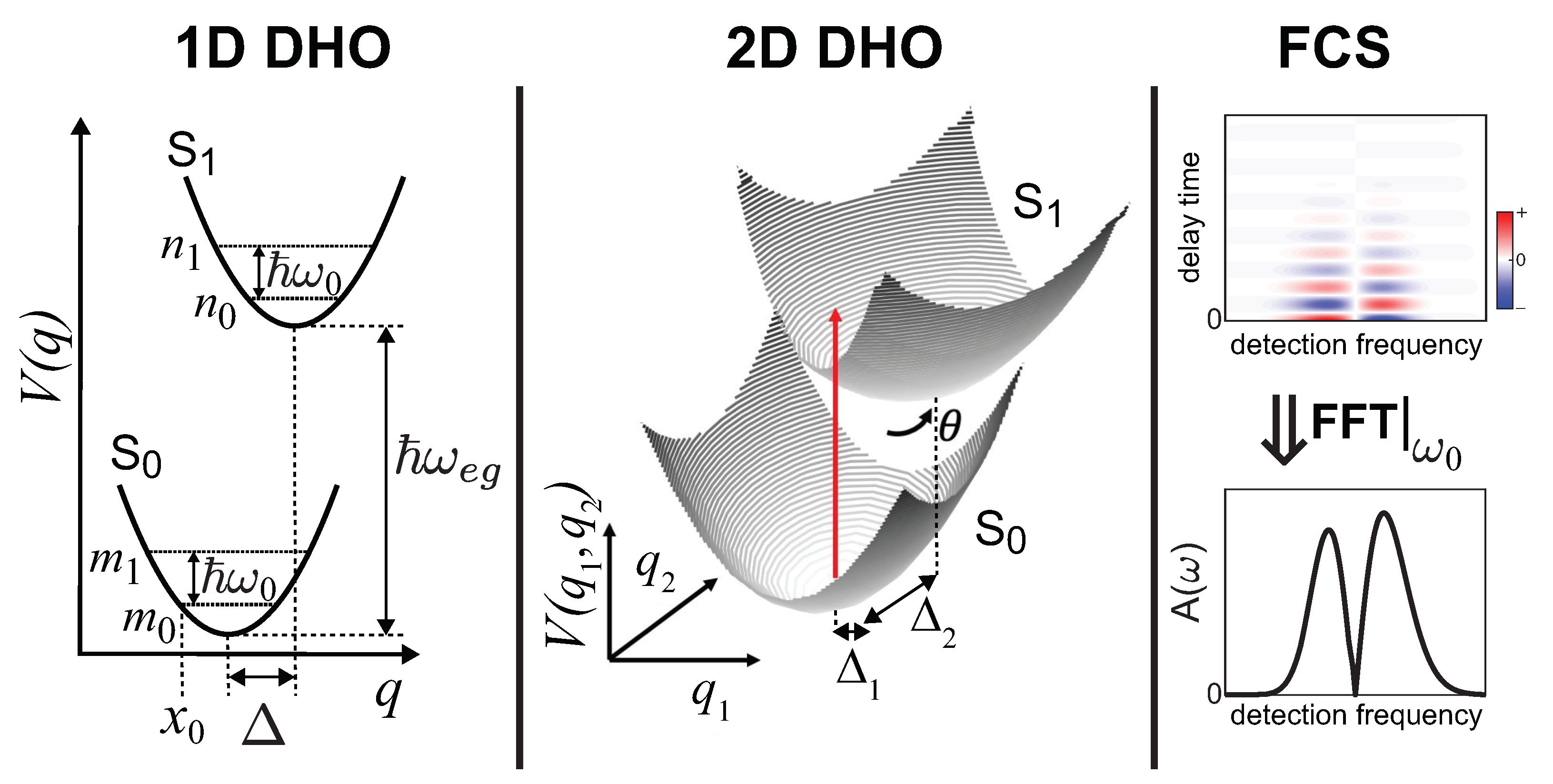In spectroscopy, one most often uses the absorption or emission of light to probe molecules near their equilibrium configurations, where nuclear motions are typically considered to be harmonic [4]. Hence, the one-dimensional displaced harmonic-oscillator model, which is shown in Figure 1, is one of the most widely used models for interpreting both steady-state and time-resolved spectra. In this model, the potential energy surface for each electronic state $S_0$ or $S_1$ is characterized as a harmonic oscillator with a certain equilibrium position, and the difference in equilibrium positions, $\Delta$, is a result of the bond-length change that arises from the deposition of energy by the light.

Impulsive spectroscopy measurements—such as transient–absorption spectroscopy—that are conducted with femtosecond laser pulses can provide a detailed view of the effects of vibronic coupling. Transient–absorption spectroscopy involves two laser pulses—a pump pulse and a probe pulse—that are focused together onto a sample, and, as the name suggests, the technique uses the change in the absorption spectrum of the sample due to its interaction with the pump pulse to acquire microscopic information about the sample [5]. The two pulses are separated by a user-controlled time-delay interval that resolves the dynamic response of the sample to the pump-pulse excitation. Transient–absorption spectroscopy can provide insight into the vibronic coupling of an isolated molecule by creating and time resolving coherent vibrational wavepacket oscillations on the ground or excited electronic state of a molecule [6,7].

An analysis method for transient–absorption spectroscopy known as femtosecond coherence spectroscopy (FCS) is beginning to reveal new insights into molecular vibronic coupling through a Fourier-domain analysis of the amplitude and phase profiles of these oscillatory signals. FCS is rooted in pioneering condensed-phase studies beginning in the 1980s [7,8,9,10,11,12,13], and FCS has gained a recent resurgence through the use of quantum-mechanical models to fit measured spectra, moving the level of analysis from qualitative to quantitative [14,15,16]. Figure 1 depicts the wavepacket oscillations and the amplitude profile created via Fourier transformation. The quantum-mechanical models for FCS are based on Franck–Condon coefficients, which are values that quantify the degree of overlap between vibrational levels of distinct electronic states. For example, the value representing the overlap between the nth (mth) vibrational sublevel of the electronic excited (ground) state is given symbolically by

$${\mathrm{FC}}_m^n(\Delta )=\int {\psi }_n(q;\Delta ){\psi }_m\left(q\right)\mathrm{d}q,$$

(1)

where $\psi \left(q\right)$ are the eigenfunctions and q represents a generic internuclear displacement. Some models lead to analytic expressions for the eigenfunctions and Franck–Condon coefficients, while in other models, these must be computed numerically. A vibrational mode that lacks a relative displacement between the two electronic states is not considered to be Franck–Condon active because the orthonormal basis of harmonic-oscillator eigenfunctions gives ${\mathrm{FC}}_m^n(\tilde{\Delta }\sim 0)\approx 0$ for $n\ne m$, meaning that excitation via light will not lead to wavepacket oscillations in most cases.

In previous work, we applied three distinct one-dimensional vibrational models to simulate and later fit measured FCS profiles, but in all instances, the microscopic values extracted from the fits were un-physically large relative to values arising from numerous prior computational and gas-phase spectroscopy studies [16]. While the purely one-dimensional vibrational models served as an important starting point, the molecules under study had dozens of normal modes, more than 10 of which were Franck–Condon active and, therefore, relevant to the measurement technique. In this work, we attempt to address the disparity between FCS measurements and theory by developing an FCS model using a two-dimensional harmonic oscillator that includes Duschinsky rotation [17] of the electronic excited-state potential-energy surface; see Figure 1. Duschinsky rotation can account for changes in the potential energy surface on the electronic excited state that create mixing between vibrational modes. Studies of Duschinksy rotation are relatively common in computational or gas-phase spectroscopy studies, but are understudied in condensed-phased spectroscopy due to a variety of complications [18].

In this contribution, we first define the FCS model and the Franck–Condon coefficients appropriate for a two-dimensional harmonic-oscillator model that includes a Duschinsky rotation angle between the two electronic states. We then present a series of simulated spectra that demonstrate the peak multiplicities, and asymmetries may offer spectral signatures for the quantification of Duschinksy rotation angles in condensed-phase spectroscopy measurements.

2. Theoretical Background

A quantum-mechanical harmonic oscillator is defined by one parameter—its angular normal-model frequency, ${\omega }_0$, which is related to the curvature by $\alpha =\sqrt{m{\omega }_0/\hslash }$, where ℏ is Planck’s constant and m represents the reduced mass. The two-dimensional harmonic oscillator eigenfunctions defined by quantum numbers $n_1$ and $n_2$ are product states that can be written as

$${\psi }_{n_1,n_2}(q_1,q_2)=\prod _{j=1}^2{N}_{n_j}{H}_{n_j}\left({\alpha }_j{q}_j\right)e^{-\frac{1}{2}{\alpha }_j^2{q}_j^2},$$

(2)

where, for each mode, the normalization constant is $N_{n_j}={\pi }^{-1/4}\sqrt{{\alpha }_j/(2^{n_j}n!)}$, and the Hermite polynomials are represented by $H_{n_j}\left(\alpha q\right)$ of order $n_j$. The Hermite polynomials explicitly involve binomial coefficients, and the normalization constants involve factorials, which leads to extensive combinatorial analysis when dealing with analytic expressions for these models.

The Franck–Condon coefficients for displaced 1D and 2D harmonic oscillator models have analytic forms [19,20,21]. For example, the FC coefficient for the 1D harmonic model when the curvatures of the ground and excited states are identical simplifies to

$${\mathrm{FC}}_m^n\left(\tilde{\Delta }\right)={(-1)}^m{e}^{-{\tilde{\Delta }}^2/4}\sqrt{\frac{n!m!}{2^{n+m}}}{\tilde{\Delta }}^{n+m}\sum _{l=0}^{\min [n,m]}{\left(-\frac{2}{{\tilde{\Delta }}^2}\right)}^l\frac{1}{l!(n-l)!(m-l)!}$$

(3)

where the unitless displacement between the equilibrium positions of the two potentials is given by $\tilde{\Delta }=\alpha \Delta$ and variables m and n index the ground-state and excited-state vibrational levels, respectively.

For the 2D model, there are now two coordinates, $q_1$ and $q_2$, each with ground-state and excited-state vibrational quantum numbers that need to be tracked, $\{m_1,m_2,n_1,n_2\}$. Here, we cast the result of Lee et al. [20] into our notation as follows:

$${\mathrm{FC}}_{m_1,m_2}^{n_1,n_2}(\tilde{\Delta },\underline{\underline{J}})=E{\left(\frac{{\alpha }_1{\alpha }_1^{\prime }{\alpha }_2{\alpha }_2^{\prime }}{A_1{A}_2{n}_1!m_1!n_2!m_2!2^{n_1+n_2+m_1+m_2}}\right)}^{1/2}\sum _{k_i=0}^{u_i}{F}_1{F}_2{F}_3,$$

(4)

where $\underline{\underline{J}}$ is the Duschinsky rotation matrix defined via a rotation angle $\theta$ as

$$\underline{\underline{J}}=\left[\begin{array}{cc}cos\left(\theta \right)& -sin\left(\theta \right)\\ sin\left(\theta \right)& cos\left(\theta \right)\end{array}\right],$$

(5)

and where the transformation from the excited-state coordinates ${\mathit{q}}^{\prime }=(q_1^{\prime },q_2^{\prime })$ to ground-state coordinates $\mathit{q}=(q_1,q_2)$ is accomplished by ${\mathit{q}}^{\prime }=\underline{\underline{J}}\mathit{q}+\Delta$. The auxiliary functions of Equation (3) are given by

$$A_1=\frac{1}{2}\left({\alpha }_1^2(1+J_{11}^2)+{\left({\alpha }_2^{\prime }\right)}^2{J}_{21}^2\right)$$

(6a)

$$B_1=\frac{1}{2A_1}\left({\left({\alpha }_1^{\prime }\right)}^2{J}_{11}{J}_{12}+{\left({\alpha }_2^{\prime }\right)}^2{J}_{21}{J}_{22}\right)$$

(6b)

$$C_1=\frac{1}{2A_1}\left({\alpha }_1^{\prime }{J}_{11}{\tilde{\Delta }}_1+{\alpha }_2^{\prime }{J}_{21}{\tilde{\Delta }}_2\right)$$

(6c)

$$A_2=\frac{1}{2}\left({\alpha }_2^2+{\left({\alpha }_2^{\prime }\right)}^2{J}_{22}^2+{\left({\alpha }_1^{\prime }\right)}^2{J}_{12}^2\right)-A_1{B}_1^2$$

(6d)

$$C_2=\frac{1}{2A_2}\left({\alpha }_1^{\prime }{J}_{12}{\tilde{\Delta }}_1+{\alpha }_2^{\prime }{J}_{22}{\tilde{\Delta }}_2-2A_1{B}_1{C}_1\right)$$

(6e)

$$E=exp\left[\left(-\frac{1}{2}{\tilde{\Delta }}_1^2+A_1{C}_1^2\right)\times \left(-\frac{1}{2}{\tilde{\Delta }}_2^2+A_2{C}_2^2\right)\right]$$

(6f)

$$F_1=\prod _{i=1}^7{a}_i^{k_i}\left(\begin{array}{c}{u}_i\\ k_i\end{array}\right)$$

(6g)

$$F_2=H_{{\eta }_1}\left(d_1\right)H_{{\eta }_2}\left(d_2\right)H_{{\eta }_3}\left(d_3\right)H_{{\eta }_4}\left(d_4\right)$$

(6h)

$$F_3={\left(\frac{2}{A_1}\right)}^{K_1/2}{\left(\frac{2}{A_2}\right)}^{K_2/2}\left(K_1-1\right)!!\left(K_2-1\right)!!,$$

(6i)

where $!!$ indicates a double factorial, and where

$$u_1=m_1,u_2=n_1,u_3=n_2,u_4=m_1-k_1,u_5=m_2,u_6=n_1-k_2,u_7=n_2-k_3$$

(7)

$$K_1=k_1+k_2+k_3,K_2=k_4+k_5+k_6+k_7,$$

(8)

where $\{K_1,K_2\}\in \left\{2\mathbb{Z}\right\}$,

$${\eta }_1=m_1-k_1-k_4,{\eta }_2=m_2-k_5,{\eta }_3=n_1-k_2-k_6,{\eta }_4=n_2-k_3-k_7$$

(9)

$$\begin{array}{cc}\hfill a_1& ={\alpha }_1,a_2={\alpha }_1^{\prime }{J}_{11},a_3={\alpha }_2^{\prime }{J}_{21},\hfill \\ \hfill a_4& =-{\alpha }_1{B}_1,a_5={\alpha }_2,a_6={\alpha }_1^{\prime }\left(J_{12}-J_{11}{B}_1\right),\hfill \\ \hfill a_7& ={\alpha }_2^{\prime }\left(J_{22}-J_{21}{B}_1\right)\hfill \end{array}$$

(10)

and

$$\begin{array}{cc}\hfill d_1& ={\alpha }_1\left(B_1{C}_2-C_1\right),d_2=-{\alpha }_2{C}_2,\hfill \\ \hfill d_3& ={\alpha }_1^{\prime }\left(J_{11}{B}_1{C}_2-J_{11}{C}_1-J_{12}{C}_2\right)+{\tilde{\Delta }}_1,\hfill \\ \hfill d_4& ={\alpha }_2^{\prime }\left(J_{21}{B}_1{C}_2-J_{21}{C}_1-J_{22}{C}_2\right)+{\tilde{\Delta }}_2.\hfill \end{array}$$

(11)

We note several clarifications. The variables $k_i$ are the indices of the summation in Equation (4). The values of $K_1$ and $K_2$ must be even, so any term with odd values of $K_1$ or $K_2$ is forced to zero. The normalized displacements use the excited-state curvatures, ${\tilde{\Delta }}_i={\Delta }_i{\alpha }_i^{\prime }$, not the ground-state curvatures, ${\alpha }_i$. The product of auxiliary functions, $F_1{F}_2{F}_3$, is a seven-dimensional quantity where each dimension is indexed by $k_i$ and then summed in Equation (4). The Hermite polynomials are of the ‘physicist’ type, $\{H_0\left(x\right)=1,H_1\left(x\right)=2x,H_2\left(x\right)=4x^2-2,\cdots \}$. Parameter $a_3$ includes a factor of $J_{21}$ that is necessary for the coordinate transformation that was missing in [20]. Finally, a coefficient computed using Equation (4) may be negative, and the formal Franck–Condon factor is the square of this coefficient.

With these Franck–Condon coefficients, we can then move to the FCS model. Before describing the model, it is instructive to first consider how the FCS profiles arise in measurements. Transient–absorption spectroscopy measurements resolve the fractional change in probe intensity induced by first photo-exciting the sample with a pump pulse as a function of the user-controlled delay between the pump and probe pulses, $\Delta I\left(\tau \right)/I_0$. In typical measurements, the probe pulse spectrum is frequency resolved in a spectrometer before detection such that the signal is given by $\Delta I(\omega ,\tau )/I_0$. In general, there are several mechanisms that can contribute to the dynamics of the signal—including energy transfer, quantum beats, quenching, intersystem crossing, radiative decay, etc.—all of which lead to a decay, growth, or oscillations in signal intensity at varying detection frequencies. For the FCS profiles, we focus only on the oscillations in the signal intensity, so we first subtract the relatively slow non-oscillatory dynamics from the detected signal, which leaves residual oscillations in the signal intensity. Figure 1 depicts illustrative residual oscillations, where the amplitude and initial phase of the oscillations vary with the detection frequency. Fourier transformation of the residuals of the signal intensity along the delay time dimension, $\tau$, produces a two-dimensional map, $M(\omega ,{\omega }_2)$, where M is a complex-valued quantity containing the amplitude and phase of the residual oscillations as a function of the detection frequency, $\omega$, and the oscillation frequency, ${\omega }_2$. Generally, the detection frequency values correspond to optical frequencies (300–600 THz), and the oscillation frequency values correspond to vibrational frequencies (1–100 THz). In many molecules, there are strong peaks at multiple oscillation frequency values that arise from the vibrational quantum beats. We are particularly interested in investigating how the amplitude of a particular oscillation varies as a function of detection frequency.

In transient–absorption measurements, the radiated signal field, $E_{\mathrm{sig}}$, interferes with the probe electric field, $E_{\mathrm{probe}}$, at the detector so that $\Delta I(\omega ,\tau )$ is given in the frequency domain by

$$\begin{array}{cc}\hfill \Delta I(\omega ,\tau )& =2\Re \left[E_{\mathrm{probe}}\left(\omega \right)E_{\mathrm{sig}}(\omega ;\tau )\right],\hfill \end{array}$$

(12)

where the signal field depends on the delay time between the pump and probe, $\tau$. It is typically assumed that the signal field is produced by a nonlinear polarization of the medium, $E_{\mathrm{sig}}\propto P_{NL}$; specifically, the polarization is the result of a third-order process such that the polarization depends on two field interactions from the pump and one from the probe.

There are standard approaches to calculating the polarization and the resulting signal field and intensity [22], one of which is referred to as the doorway–window formalism [9], which is appropriate in the limit in which the pump and probe pulses are well separated in time. The doorway–window method has a relatively intuitive physical interpretation [23]: The pump pulse prepares the sample in a non-equilibrium state, which then evolves, and the probe pulse acts as a window to the state of the sample. This allows one to introduce models of the dynamics of interest, which, in the present work, are vibrational quantum beats.

In the doorway–window approach used here, the pump pulse creates a wavepacket in the excited electronic state that can be described by a density matrix given by

$$\rho \left(\tau \right)=\sum _{\{n,n^{\prime }\}}^{N,N}{\mathrm{FC}}_0^{\left\{n\right\}}{\mathrm{FC}}_0^{*,\left\{n^{\prime }\right\}}{e}^{-i(E_{\left\{n^{\prime }\right\}}-E_{\left\{n\right\}})\tau /\hslash }\left|e,\left\{n\right\}\right.〉\left.〈e,\left\{n^{\prime }\right\}\right|,$$

(13)

where ${}^{*}$ represents a complex conjugate, $\tau$ is the time delay after initial excitation, $\left|e,\left\{n\right\}\right.〉$ represents the state of the $\left\{n\right\}$th vibrational level on the electronic excited state with energy $E_{\left\{n\right\}}$, and N vibrational levels are assumed. The curly braces indicate that the model may have multiple dimensions, and the primed index indicates a second, independent vibrational state. In deriving this expression, we have assumed that the transition-dipole moment is independent of the nuclear displacement and that the pump pulse has infinite bandwidth, which is appropriate for situations where the pump-pulse bandwidth is broader than the sample absorption. The probe pulse provides a “window” to the state of the evolving wavepacket. We use a window operator of the form [15,24]:

$$W\left(\omega \right)=\sum _{\{n,n^{\prime }\}}^{N,N}\left|e,\left\{n\right\}\right.〉\left.〈e,\left\{n^{\prime }\right\}\right|\sum _{\left\{m\right\}}^N{\mathrm{FC}}_{\left\{m\right\}}^{\left\{n\right\}}{\mathrm{FC}}_{\left\{m\right\}}^{*,\left\{n^{\prime }\right\}}\left[\frac{1}{\omega -{\omega }_{\{n^{\prime },m\}}+i\gamma /2}-\frac{1}{\omega -{\omega }_{\{n,m\}}-i\gamma /2}\right],$$

(14)

where $\omega$ is the detection frequency variable, the primed indices indicate the involvement of a second, independent excited-state vibrational state, the curly braces indicate the collective dimensions of the quantum-mechanical model, and $\gamma$ is a phenomenological line-broadening parameter capturing the microscopic solvation dynamics of the system [22]. The calculated transient absorption signal $(S\propto \Delta I)$ as a function of detection frequency $\omega$ and the delay between the pump and probe $\tau$ can be found from

$$S(\omega ,\tau )=\mathrm{Tr}\left[W\left(\omega \right)\rho \left(\tau \right)\right].$$

(15)

In determining FCS profiles, we focus on the amplitude and phase of the oscillations in the signal intensity as a function of detection frequency; therefore, we define $\tilde{S}(\omega ,{\omega }_2)={\mathcal{F}}_{\tau }\left[S(\omega ,\tau )\right]$, where ${\mathcal{F}}_{\tau }$ is a Fourier transform along the delay time axis. This is analogous to the analysis of measurements wherein one takes a Fourier transform of the intensity oscillations along the delay time axis. This model assumes that the transition-dipole moment has no dependence on the coordinate, and it neglects more complicated relaxation mechanisms, such as nonadiabatic coupling or energy transfer. The general frequency-dependent signal based on the Franck–Condon coefficients is given by

$$\begin{array}{cc}\hfill \tilde{S}(\omega ,{\omega }_2)=& \sum _{\{n,n^{\prime },m\}}^N{\mathrm{FC}}_{\left\{m\right\}}^{\left\{n\right\}}{\mathrm{FC}}_{\left\{m\right\}}^{*,\left\{n^{\prime }\right\}}{\mathrm{FC}}_{\left\{0\right\}}^{\left\{n\right\}}{\mathrm{FC}}_{\left\{0\right\}}^{*,\left\{n^{\prime }\right\}}\left[\frac{1}{\omega -{\omega }_{\{n^{\prime },m\}}+i\gamma /2}-\frac{1}{\omega -{\omega }_{\{n,m\}}-i\gamma /2}\right]\hfill \\ \hfill & \times 2\pi \delta \left({\omega }_2-(E_{\left\{n^{\prime }\right\}}-E_{\left\{n\right\}})/\hslash \right),\hfill \end{array}$$

(16)

where ${\omega }_2$ is the oscillation frequency variable that arises from Fourier transformation of the measured oscillations in a signal intensity [15]. This expression arose from a doorway–window treatment of the coherent wavepackets produced by broadband laser pulses in transient–absorption spectroscopy [23,25,26]. In a transient–absorption spectroscopy measurement, the vibrational oscillations dephase, often on picosecond timescales, which adds a finite width to the peak along the oscillation frequency axis, ${\omega }_2$.

In this work, we study oscillations at the fundamental frequency of one mode. Without loss of generality, we study the excited-state wavepacket oscillations exclusively at the frequency of the mode on the ground-state coordinate $q_1$, which is ${\omega }_{0_1}$, by integrating over a small spectral window near ${\omega }_2={\omega }_{0_1}$ to produce a mode-specific FCS profile $M(\omega ,{\omega }_{0_1})={\int }_{{\omega }_{0_1}-\delta \omega }^{{\omega }_{0_1}+\delta \omega }\tilde{S}(\omega ,{\omega }_2)d{\omega }_2$. This constrains the indices in the sums to $n_1^{\prime }=n_1+1$ and $n_2^{\prime }=n_2$. This model requires the product of the four coefficients, ${\mathrm{FC}}_{m_1,m_2}^{n_1,n_2}{\mathrm{FC}}_{m_1,m_2}^{*,n_1^{\prime },n_2^{\prime }}{\mathrm{FC}}_{0,0}^{n_1,n_2}{\mathrm{FC}}_{0,0}^{*,n_1^{\prime },n_2^{\prime }}$, with the constraints on $n_1^{\prime }$ and $n_2^{\prime }$. Hence, the relevant expression is given by

$$\begin{array}{cc}\hfill M(\omega ,{\omega }_{0_1})=& \sum _{\begin{array}{c}{n}_1,n_2,\\ m_1,m_2\end{array}}^N{\mathrm{FC}}_{m_1,m_2}^{n_1,n_2}{\mathrm{FC}}_{m_1,m_2}^{n_1+1,n_2}{\mathrm{FC}}_{0,0}^{n_1,n_2}{\mathrm{FC}}_{0,0}^{n_1+1,n_2}\hfill \\ \hfill & \times \left[\frac{1}{\omega -{\omega }_{n_1+1,n_2,m_1,m_2}+i\gamma /2}-\frac{1}{\omega -{\omega }_{n_1,n_2,m_1,m_2}-i\gamma /2}\right],\hfill \end{array}$$

(17)

where, because the Franck–Condon coefficients are real-valued, we drop the complex-conjugate notation. With these considerations, the simulations of $M(\omega ,{\omega }_{0_1})$ with six Franck–Condon coefficients for each index required about 30 s of computation time on a standard personal computer. As confirmation, we compared several arbitrary Franck–Condon coefficients and the spectra simulated using Equation (17) to those arising from explicit integration of real-space eigenfunctions and found them to be identical.

3. Results and Discussion

The purpose of this work is to study the effect of a Duschinsky rotation on spectral features in simulated FCS. In prior work, we found that all 1D models produced a sharp node separating two peaks of differing amplitudes, such as those shown in Figure 1. The 1D models generally predict, at most, a weak asymmetry between the peak amplitudes in the simulated FCS, and they predict that the peak at lower detection frequencies is always weaker, assuming physically relevant conditions. By contrast, FCS arising from measurements often show a strong asymmetry. Specifically, in many measurements, the peak at a lower detection frequency has a substantially reduced amplitude relative to that of the peak at a higher detection frequency. We found that fitting the measured FCS amplitude profiles using the 1D models required un-physically large parameters [27]. Hence, here, we aim to simulate FCS with the 2D model and identify a distinct signature that will allow us to quantify the rotation angle value, $\theta$. We also aim to demonstrate that the model can produce peaks with strongly asymmetric peak amplitudes. In both simulations and measurements, $M(\omega ,{\omega }_{0_1})$ is a complex-valued quantity that has both amplitude and phase profiles. In prior works, we found it most productive to focus on the amplitude profiles. Therefore, the figures display the amplitude profiles defined by

$$A\left(\omega \right)=\left|M(\omega ,{\omega }_{0_1})\right|.$$

(18)

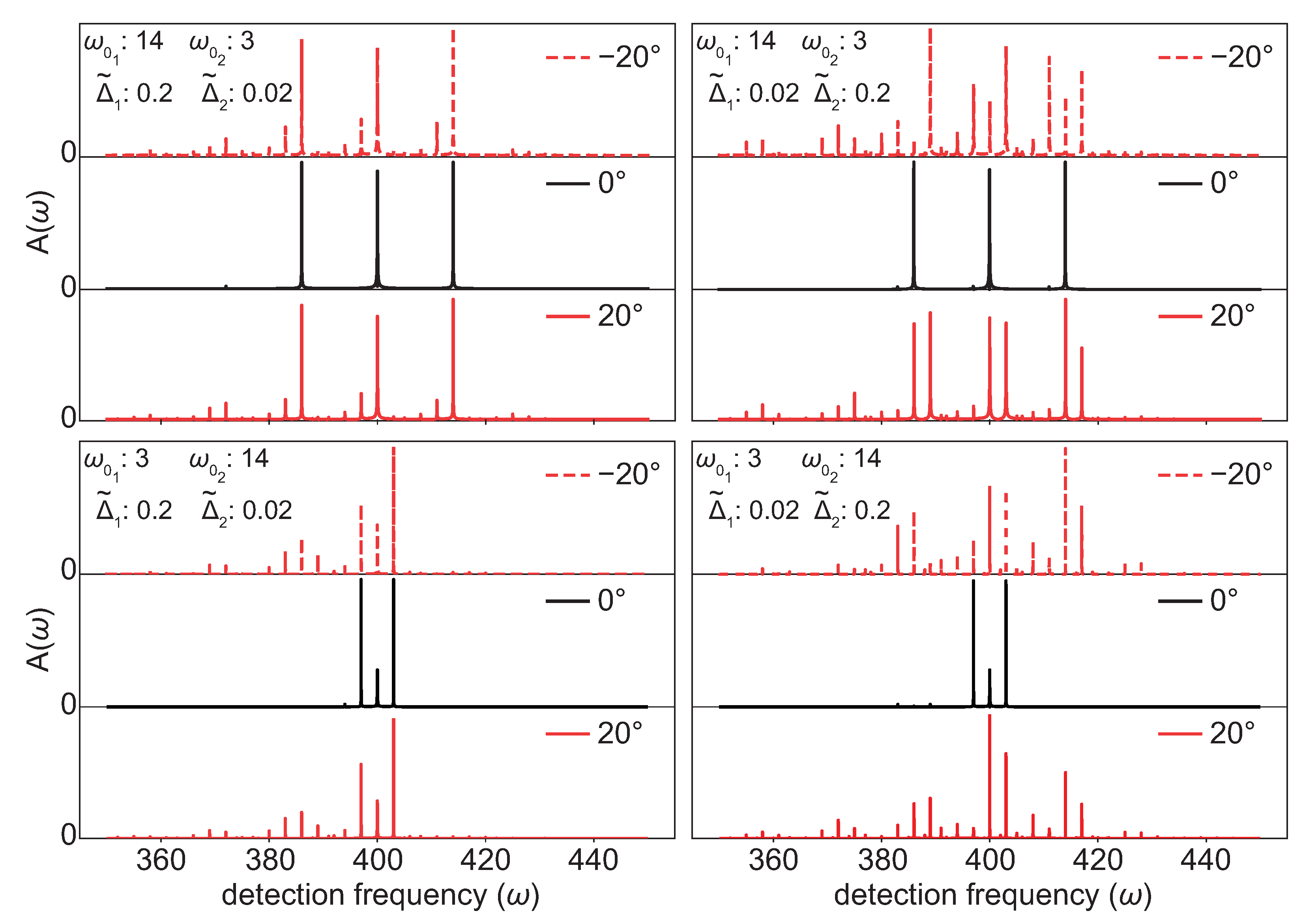
As a first step, we set the line-broadening parameter to a value small enough to discern individual transitions, $\gamma /{\omega }_{0_1}=0.001$. This could, for example, represent a gas-phase spectroscopy measurement, which would have sharp transitions due to the lack of solvation [22]. By identifying each transition in the spectrum, we can identify changes in the multiplicity (peak splittings) as the Duschinsky angle varies. Because we inspect only the FCS of mode 1, which we label as the ‘fundamental’ mode, we must simulate several cases, depending on the relative frequency and displacement of mode 2, which we label as the ‘spectator’ mode. There are four cases for capturing the possible relative values of the frequency and displacement parameters. In each of those four cases, we examine the spectra for rotation angles of $\{-{20}^{\circ },0^{\circ },+{20}^{\circ }\}$. Computational studies indicate that rotations can have nearly any angle, and hence, the values of $\pm {20}^{\circ }$ demonstrate the perturbative effect of the mixing rather than complete rotation.

The panel in the upper left of Figure 2 is the case of ${\omega }_{0_1}>{\omega }_{0_2}$ and ${\tilde{\Delta }}_1>{\tilde{\Delta }}_2$, when the spectator mode has a frequency and displacement that are far less than those of the fundamental mode. The simulated FCS reveal that in the spectrum with no rotation, there are three strong peaks with a separation of ${\omega }_{0_1}$, which fits the expectations from our prior work [15]. Through close inspection, one can notice that the peak at $\omega ={\omega }_{eg}$ has an amplitude that is slightly less than those of the peaks at $\omega ={\omega }_{eg}\pm {\omega }_{0_1}$. The $\pm {20}^{\circ }$ spectra are almost identical to each other: The spectator mode causes the main central peak to slightly decrease in amplitude and causes each main peak to become a series of progressively weaker peaks. This peak multiplicity is similar to a ‘triplet of triplets’ pattern found in nuclear magnetic resonance spectroscopy [28]. The peak spacing of each progression is ${\omega }_{0_2}$, and the additional peak progressions are dominantly shifted towards lower detection frequencies.

The lower-left panel of Figure 2 is the case of ${\omega }_{0_1}<{\omega }_{0_2}$ and ${\tilde{\Delta }}_1>{\tilde{\Delta }}_2$, when the spectator mode has a frequency greater than and a displacement less than those of the fundamental mode. The results are similar to those in the previous case: The 0${}^{\circ }$ spectrum is similar to a single-mode spectrum with dominant peaks separated by ${\omega }_{0_1}$, and the $\pm {20}^{\circ }$ spectra are nearly identical to each other. In each spectrum, the amplitude of the peak at $\omega ={\omega }_{eg}-{\omega }_{0_1}$ is reduced and additional clusters of peaks appear. The peaks within a cluster are separated by ${\omega }_{0_1}$, unlike the previous case, in which ${\omega }_{0_1}>{\omega }_{0_2}$. The center frequency of each cluster is separated by ${\omega }_{0_2}$, and the progression of clusters all shifts towards lower detection frequencies. This case is unique among the simulations because it is the only case in which—regardless of rotation angle—no peaks appear when $\omega >{\omega }_{eg}$, except for the single peak at ${\omega }_{eg}+{\omega }_{0_1}$.

In the right column of Figure 2, the fundamental mode has a small displacement, the spectator mode has a large displacement (${\tilde{\Delta }}_1<{\tilde{\Delta }}_2$), and the spectra at the fundamental frequency are more sensitive to rotations because this causes mixing with a significantly displaced mode. In the upper-right panel for ${\omega }_{0_1}>{\omega }_{0_2}$, the fundamental frequency is large and the spectator mode frequency is small. Because the displacement of the spectator mode is large, it even makes a contribution in the $0^{\circ }$ spectrum, an effect that we had not previously observed with 1D models. The three dominant peaks are spaced by ${\omega }_{0_1}$ and look similar to those in the panel on the left, but three weak peaks are visibly shifted by ${\omega }_{0_2}$ below each of the dominant peaks. Adding a nonzero rotation introduces clusters of peaks similar to those in the left column. In contrast to the left column, the $+{20}^{\circ }$ and $-{20}^{\circ }$ spectra are quite distinct. For example, consider the central peak at $\omega ={\omega }_{eg}$. For both $\pm {20}^{\circ }$, the central peak splits into three peaks that are separated by ${\omega }_{0_2}$. For $+{20}^{\circ }$, the central peak and the peak shifted to a higher frequency are of roughly equal amplitudes, and the peak shifted to a lower frequency is very weak. For a $-{20}^{\circ }$ rotation, the central peak is the weakest of the three. In addition to the asymmetry between the $\pm {20}^{\circ }$ spectra, we note that unlike the left column, there is now significant amplitude in peaks shifted toward higher detection frequencies.

Finally, in the lower-right panel, we show the case of ${\omega }_{0_1}<{\omega }_{0_2}$ and ${\tilde{\Delta }}_1<{\tilde{\Delta }}_2$. Similarly to the upper-right panel, the $\pm {20}^{\circ }$ spectra produce rather distinct FCS profiles. Now, there are entire clusters of peaks shifted to higher frequencies, where the shift in each cluster is, of course, ${\omega }_{0_2}$. Like all other cases in which the rotation angle is $0^{\circ }$, here too, this spectrum is identical to that produced by simulations using a 1D model.

In summary, these simulations indicate that, as expected, when the rotation angle is zero, the simulations are nearly identical to those that would arise in simulations using 1D models. The primary signature of a nonzero rotation angle is strong peak splitting at the frequency of the coupled mode. This effect is particularly pronounced when the displacement of the spectator mode is much greater than the displacement of the fundamental mode, regardless of relative frequencies or the sign of rotation angle. Because we are displaying only the amplitude profiles, $A\left(\omega \right)$, we are blind to the phase of each peak in Figure 2. While in prior works, we examined the phase profiles, $\varphi \left(\omega \right)$, directly [15], they can be extremely complicated. Instead, it is more productive to examine the interference effects that arise when the peaks are broad and overlapping.

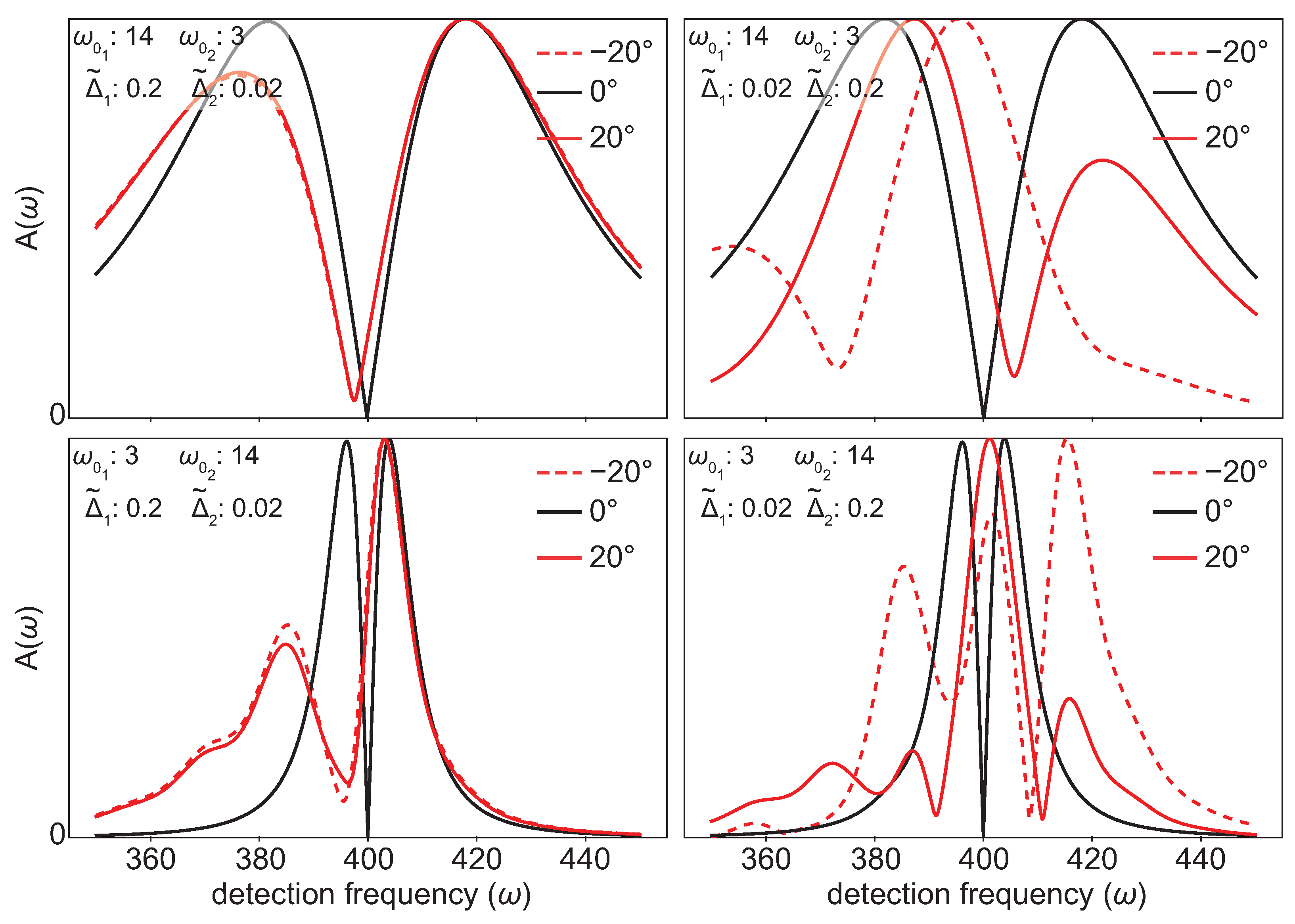
Therefore, we performed simulations for the same four cases as in Figure 2, where the only change was the value of $\gamma /{\omega }_{0_1}$, and we display the results in Figure 3. Increasing $\gamma$ causes the lines to broaden and overlap. At most detection frequencies, the overlapping lines interfere constructively. At the main “node”, the lines interfere destructively. For consistency with prior work, we choose here to define the broadening in terms of the fundamental mode and choose $\gamma /{\omega }_{0_1}=4$ for all four cases. In the calculation of two-mode FCS profiles, our choice of defining $\gamma$ in terms of the fundamental mode has consequences for the shape of the calculated profiles. In the top row of Figure 1, ${\omega }_{0_1}>{\omega }_{0_2}$, and $\gamma$ is larger than the spacing between either mode, so no distinct peaks are observed. In the bottom row, $\gamma$ is smaller than the spectator frequency mode spacing, and distinct peaks are still observably separated by ${\omega }_{0_2}$. This specific difference between the top and bottom rows is merely a consequence of the ambiguity in defining $\gamma$ in a consistent manner for two-mode FCS profiles.

In all four cases, $0^{\circ }$ rotation produces an FCS profile that looks very similar to the FCS profile for a single-mode calculation. There are also two trends that affect all four cases for the nonzero rotation angle. The first is a pronounced ‘softening’ of the node, which arises from interference among the new peaks introduced from the nonzero rotation, which yields an incomplete cancellation. The second is a shift in the detection frequency at which the node is deepest, which arises from the change in amplitude of the transitions, observed on an individual level in Figure 2.

To examine the effects of a nonzero rotation angle in more detail, we begin in the left column, where the displacement of the fundamental mode is relatively large compared to that of the spectator mode, $({\tilde{\Delta }}_1>{\tilde{\Delta }}_2)$. When $\gamma$ is very small (Figure 2) in these two cases, rotating to $\pm {20}^{\circ }$ adds additional lines or clusters of lines shifted by the spectator mode frequency in the direction of lower detection frequencies. Consequently, the high-frequency peak of the corresponding spectrum in Figure 3 is nearly unchanged; the changes that arise from the rotation are observed primarily in the low-detection-frequency portion of the profile. The low-detection-frequency peaks for both cases in the left column of Figure 3 have a reduced amplitude and are broadened. In the upper-left panel, the spectator mode spacing is small; therefore, the effects are less pronounced. In the lower-left panel, the spectator mode is a high frequency and the spacing between clusters of lines—which arise from the mode mixing—is large compared to the spacing between lines in the fundamental mode. This increases the broadening toward lower detection frequencies and increases the asymmetry between the relative height of the high- and low-detection-frequency peaks in the spectra. Similarly to the spectra in Figure 2, rotations in either direction produce nearly identical spectra in Figure 3 for these two cases.

Next, we examine the cases in the right column of Figure 3, which show the effect of rotation when the fundamental mode has a small displacement and the spectator mode has a large displacement. For these cases in Figure 2, we observed that nonzero rotation angle introduced new peaks—and clusters of peaks—shifted to both lower and higher detection frequencies. The consequences of the interference among these new peaks are revealed in Figure 3, where we observe significant changes in not only the low-frequency peaks, but also the high-frequency primary peaks in the $0^{\circ }$ spectrum. In nearly all simulations, the spectrum is severely distorted relative to its corresponding $0^{\circ }$ spectrum. In the top-right case (${\omega }_{0_1}>{\omega }_{0_2}$, ${\tilde{\Delta }}_1<{\tilde{\Delta }}_2$), the $-{20}^{\circ }$ spectrum has a massive red shift in the node location and an approximately 50% change in the relative amplitudes, and the $+{20}^{\circ }$ spectrum is even more unusual, showing a blueshifted node and a 50% change in the relative amplitudes, but with the previously unobserved effect that the lower-frequency peak has a greater amplitude. In the bottom-right case (${\omega }_{0_1}<{\omega }_{0_2}$, ${\tilde{\Delta }}_1<{\tilde{\Delta }}_2$), the $-{20}^{\circ }$ spectrum now has three peaks of varying heights and two nodes: a blueshifted primary node, a secondary node to the red, and a peak where the $0^{\circ }$ spectrum had a node. The $+{20}^{\circ }$ spectrum shows at least four peaks with three regions of low amplitude. By comparing this with the corresponding spectrum in Figure 2, the regions near 390 and 410 THz are nodes due to the interference of overlapping out-of-phase transitions. The region at 380 THz appears to be a dip arising from the absence of transitions at this detection frequency. Again, there is a peak at the detection frequency where the $0^{\circ }$ spectrum had a node.

The spectra in Figure 3 reveal that a nonzero Duschinsky rotation angle causes distortions that range from subtle to severe, depending primarily on the relative displacements of the two modes of the 2D model. When the fundamental mode has a larger displacement than the spectator mode, the effects are subtle changes in the relative peak heights, softening and frequency-shifting of the node location, and, in some cases, changes in the peak widths. By contrast, when the spectator mode has a larger displacement than the fundamental mode, the changes in the FCS profiles are dramatic. The nonzero rotation generates multiple new peaks and nodes in both the blue and red frequencies and even previously unobserved changes in the relative peak heights.

4. Conclusions

In this contribution, we have presented a 2D harmonic-oscillator model for use in simulations of femtosecond coherence spectra. The expressions for the Franck–Condon coefficients are the crucial element in these simulations, and the coefficients involve significant combinatorics. The model includes the possibility of a rotation between the two electronic states, which is known as Duschinsky rotation. By examining the spectra that arise purely from oscillations at one of the mode frequencies, we have shown that when the Duschinksy rotation angle is zero, the simulations are nearly identical to those arising from the corresponding 1D model. By contrast, a nonzero rotation angle yields new transitions or clusters of transitions that can interfere to cause a range of changes. In some parameter sets, the effects of nonzero rotation angle were subtle, whereas in other parameter sets, the nonzero rotation angle caused quite dramatic changes in the spectrum. This model can be used to fit measured spectra that previously produced un-physical values when fitted by 1D models. Future work could include revisiting unequal curvature cases, which we have not examined, or could make comparisons with quantum-chemical computations of Duschinsky rotations.