Mathematical Models for Population Growth with Variable Carrying Capacity: Analytical Solutions

Abstract

A general population model with variable carrying capacity consisting of a coupled system of nonlinear ordinary differential equations is proposed, and a procedure for obtaining analytical solutions for three broad classes of models is provided. A particular case is when the population and carrying capacity per capita growth rates are proportional. As an example, a generalised Thornley–France model is given. Further examples are given when the growth rates are not proportional. A criterion when inflexion may occur is also provided, and results of numerical simulations are presented.

1. Introduction

The logistic model has been extensively used to study the cause and effect relationship between the ‘carrying capacity’ (i.e., the population size that available resources can support) and the population size. See, for instance, the references in Brauer & Castillo-Chávez [1], Gotelli [2], Pastor [3], as well the seminal papers by Verhulst [4] and Pearl & Reed [5].

It is typically assumed that the carrying capacity does not vary with time and, therefore, the logistic model exhibits a sigmoidal shape when the population size is plotted as a function of time. However, many phenomena such as human population growth exhibit more complex behaviours, unlike population species grown in laboratory cultures, for example. Thus, it is of theoretical and practical interest to investigate mathematical models that incorporate variable carrying capacities. One of the main objectives of studying such models is to explore how different functional forms of the carrying capacity influence the dynamics of the population variable and its long-term behaviour.

Meyer [6] and Meyer & Ausubel [7] studied a bi-logistic model derived from a logistic model but with a sigmoidal time-dependent carrying capacity. Cohen [8] proposed a human population growth model with a variable carrying capacity that is a function of the population size itself. The aforementioned models make the case that the inclusion of a variable carrying capacity is more reflective of the human condition.

Safuan et al. [9] proposed a coupled system of ordinary differential equations (ODEs) to describe the interaction between the population and its carrying capacity. The model they considered does not require prior knowledge of the carrying capacity, nor does it impose constraints on the initial conditions. Assuming a special form of the carrying capacity in the logistic equation, the same authors obtained an analytical solution in series form [10].

As pointed out by Cohen [8], there is no consensus with regards to appropriate models for human carrying capacity. However, most would accept that human carrying capacity is influenced by food availability, amongst other factors. Hopfenberg [11] postulated that food production data are the sole variable that influences human carrying capacity, and a simple linear relationship between human carrying capacity and the food production index is assumed. More recently, Zulkarnaen & Rodrigo [12] proposed three classes of human population dynamical models of logistic type where the carrying capacity is a function of the food production index. They employed an integration-based parameter estimation technique [13] to derive explicit formulas for the model parameters. Using actual population and food production index data, the results of numerical simulations of their models suggested that an increase in food availability implies an increase in carrying capacity, but the carrying capacity is ‘self-limiting’ and does not increase indefinitely.

Thornley & France [14] proposed an ‘open-ended’ form of the logistic equation by considering a system of two ODEs representing the coupled processes of growth and development. Their model is ‘open-ended’ in the sense that dynamic changes in nutrition and environment can influence growth and development, which, in turn, may affect the asymptotic carrying capacity value. Subsequently, Thornley et al. [15] found an analytical solution to the Thornley–France model in the case of constant parameters. The solution of the system of ODEs is expressed in terms of the solution of a single ODE of power-law logistic type, also referred to as the $\theta$-logistic model, which frequently arises in ecology and elsewhere [16]. A related article by Wu et al. [17] formulated the variable carrying capacity by exploring a resource dynamic-based feedback mechanism underlying the population growth models. The inclusion of variable carrying capacities in interacting species such as in predator–prey models have been considered in Al-Moqbali et al. [18], Al-Salti et al. [19].

Power-law logistic models have been investigated by von Bertalanffy [20] and Richards [21]. The principal (nonnegative) parameter of these models is denoted by $\theta$. The Gompertz model and the logistic model are recovered when $\theta =0$ and $\theta =1$, respectively. Larger values of $\theta$ behave like a logistic model but with an increasingly sharper cessation of growth as the asymptote (i.e., the constant carrying capacity limit) is approached [15]. As a fraction of the asymptote, inflexion can occur over the range from $\frac{1}{\mathrm{e}}$ (Gompertz) through $\frac{1}{2}$ (‘ordinary’ logistic) and then to 1 (for large $\theta$). Determining the point where inflexion takes place can be especially important when fitting the model to actual data that exhibit a sigmoidal trend. See Banks [22] for a detailed analysis of the $\theta$-logistic model. More recently, Albano et al. [23] considered a general growth curve that includes the Malthus, Richards, Gompertz and other models. Their generalised model is essentially a Bernoulli ODE, which is well known to be analytically tractable. They investigated the analytical and numerical properties of the solution as the parameters varied.

Here we propose a general population model with a variable carrying capacity, which includes the Thornley–France [14], Safuan–Jovanoski–Towers–Sidhu [9] and Meyer–Ausubel [7] models as special cases. Moreover, when the carrying capacity is kept constant, the proposed model system reduces to a single ODE population model and recovers the Gompertz, ‘ordinary’ logistic and $\theta$-logistic models, amongst others. The idea is to extract the essential properties of such models without getting ‘bogged down’ by particular cases. We provide a procedure for obtaining, when possible, the analytical solution of this general population model. Different models can then be chosen depending on the particular phenomenon being studied. An important tractable special case is when the per capita growth rates of the population and carrying capacity are proportional to each other. We give a criterion for when inflexion may occur. Several illustrative examples are also provided.

2. Population Models with Variable Carrying Capacities

Consider the initial value problem (IVP)

$$\frac{\mathrm{d}N}{\mathrm{d}t}=Nf(N,K),\frac{\mathrm{d}K}{\mathrm{d}t}=Kg(N,K),N\left(0\right)=N_0,K\left(0\right)=K_0,$$

(1)

where $N\left(t\right)$ and $K\left(t\right)$ are the population and carrying capacity, respectively, at time t. The initial values $N_0$ and $K_0$ are positive and given. Let f and g be sufficiently smooth bivariate functions on ${\mathbb{R}}_{+}\times {\mathbb{R}}_{+}$, where ${\mathbb{R}}_{+}=(0,\infty )$. Denote by $D_j$, where $j=1,2$, the partial derivative with respect to the independent variable in the jth position. We assume that the population per capita growth rate $\frac{1}{N}\frac{\mathrm{d}N}{\mathrm{d}t}$ decreases with increasing population ($D_{1}f(x,y)<0$) and increases with increasing carrying capacity ($D_{2}f(x,y)>0$). As for the signs of $D_{1}g(x,y)$ and $D_{2}g(x,y)$, it is not obvious what these should be since the behaviour of the carrying capacity per capita growth rate $\frac{1}{K}\frac{\mathrm{d}K}{\mathrm{d}t}$ may depend on the particular population species.

When g is identically zero, then $K\left(t\right)=K_0$ and (1) reduces to

$$\frac{\mathrm{d}N}{\mathrm{d}t}=Nf(N,K_0),N\left(0\right)=N_0.$$

A well-known example is the $\theta$-logistic model [22]

$$f(N,K_0)=\frac{r}{\theta }\left[1-{\left(\frac{N}{K_0}\right)}^{\theta }\right],$$

where $r>0$ is the intrinsic growth rate, and $\theta >0$ is a parameter related to the point of inflexion of the solution. The case $\theta =1$ gives the ‘ordinary’ logistic model. In the limit as $\theta \to 0^{+}$, the $\theta$-logistic model reduces to the Gompertz model [24]

$$f(N,K_0)=rlog\left(\frac{K_0}{N}\right).$$

In the case of a variable carrying capacity, the Thornley–France model [14] takes the form

$$\begin{array}{c}\hfill f(N,K)=a\left(1-\frac{N}{K}\right),g(N,K)=-b\left(1-\frac{N}{K}\right),\end{array}$$

(2)

where $a,b>0$. Note that $D_{1}g(x,y)>0$ and $D_{2}g(x,y)<0$. Safuan et al. [9] proposed the model

$$\begin{array}{c}\hfill f(N,K)=a\left(1-\frac{N}{K}\right),g(N,K)=b-cN,\end{array}$$

(3)

where $a,b,c>0$. Here we see that $D_{1}g(x,y)<0$ and $D_{2}g(x,y)=0$. Meyer [6] and Meyer & Ausubel [7] assumed that

$$\begin{array}{c}\hfill f(N,K)=a\left(1-\frac{N}{K}\right),g(N,K)=b-cK,\end{array}$$

where $a,b,c>0$. This time, $D_{1}g(x,y)=0$ and $D_{2}g(x,y)<0$.

2.1. Construction of Analytically Tractable Population Models with Variable Carrying Capacities

Suppose that there exists a positive $C^1$-function F such that $y=F\left(x\right)$ solves the IVP

$$yg(x,y)\mathrm{d}x-xf(x,y)\mathrm{d}y=0,y=K_0\mathrm{when}x=N_0.$$

(4)

Define

$$G\left(x\right)={\int }_{N_0}^x\frac{1}{zf(z,F(z\left)\right)}\mathrm{d}z.$$

(5)

We claim that

$$G\left(N\right(t\left)\right)=t,K\left(t\right)=F\left(N\right(t\left)\right)$$

(6)

gives the formal solution of (1) in implicit form. Indeed, (4) and (6) imply that

$$F^{\prime }\left(x\right)=\frac{F\left(x\right)g(x,F(x\left)\right)}{xf(x,F(x\left)\right)},F^{\prime }\left(N\left(t\right)\right)=\frac{K\left(t\right)g\left(N\right(t),K(t\left)\right)}{N\left(t\right)f\left(N\right(t),K(t\left)\right)}.$$

Implicitly differentiating $G\left(N\right(t\left)\right)=t$ with respect to t yields

$$1=G^{\prime }\left(N\left(t\right)\right)N^{\prime }\left(t\right)=\frac{1}{N\left(t\right)f\left(N\right(t),K(t\left)\right)}{N}^{\prime }\left(t\right)$$

or $\frac{\mathrm{d}N}{\mathrm{d}t}=Nf(N,K)$. Hence

$$K^{\prime }\left(t\right)=F^{\prime }\left(N\left(t\right)\right)N^{\prime }\left(t\right)=\frac{K\left(t\right)g\left(N\right(t),K(t\left)\right)}{N\left(t\right)f\left(N\right(t),K(t\left)\right)}{N}^{\prime }\left(t\right)=K\left(t\right)g(N\left(t\right),K\left(t\right))$$

or $\frac{\mathrm{d}K}{\mathrm{d}t}=Kg(N,K)$. It is clear that $G\left(N\left(0\right)\right)=G\left(N_0\right)=0$ and $K\left(0\right)=F\left(N\left(0\right)\right)=F\left(N_0\right)=K_0$. This proves the claim. Therefore, the task of finding an analytical solution of (1) essentially reduces to solving the first-order ODE (4).

2.2. Determination of Inflexion Points for the Population Species Variable

Before we consider some examples, let us first investigate where inflexion may occur for the population species variable. As mentioned previously, this is particularly relevant during model fitting. Using (6) and differentiating the first ODE in (1) with respect to t, we have

$$\begin{array}{c}\hfill \frac{{\mathrm{d}}^{2}N}{\mathrm{d}{t}^2}=[f(N,F\left(N\right))+N{D}_{1}f(N,F\left(N\right))+N{D}_{2}f(N,F\left(N\right))F^{\prime }\left(N\right)]\frac{\mathrm{d}N}{\mathrm{d}t}.\end{array}$$

Therefore, inflexion for the function N may occur at some positive root $N^{*}$ of the equation

$$H\left(z\right)=f(z,F\left(z\right))+z{D}_{1}f(z,F\left(z\right))+z{D}_{2}f(z,F\left(z\right))F^{\prime }\left(z\right)=0.$$

(7)

If this occurs, it will be when $t=t^{*}$, where

$$t^{*}=G\left(N\left(t^{*}\right)\right)=G\left(N^{*}\right)={\int }_{N_0}^{N^{*}}\frac{1}{zf(z,F(z\left)\right)}\mathrm{d}z.$$

(8)

2.3. First Class of Analytically Tractable Models: f and g Are Proportional

Suppose that there exists $\alpha \in \mathbb{R}\setminus \left\{0\right\}$ such that $g(x,y)=\alpha f(x,y)$. This basically assumes that the per capita growth rates $\frac{1}{N}\frac{\mathrm{d}N}{\mathrm{d}t}$ and $\frac{1}{K}\frac{\mathrm{d}K}{\mathrm{d}t}$ are proportional. Then (4) and (5) give

$$y=F\left(x\right)=K_0{N}_0^{-\alpha }{x}^{\alpha },G\left(x\right)={\int }_{N_0}^x\frac{1}{zf(z,K_0{N}_0^{-\alpha }{z}^{\alpha })}\mathrm{d}z,$$

respectively. From (6) we obtain the exact solution

$${\int }_{N_0}^{N\left(t\right)}\frac{1}{zf(z,K_0{N}_0^{-\alpha }{z}^{\alpha })}\mathrm{d}z=t,K\left(t\right)=K_0{N}_0^{-\alpha }{\left[N\left(t\right)\right]}^{\alpha }$$

(9)

of the system (1).

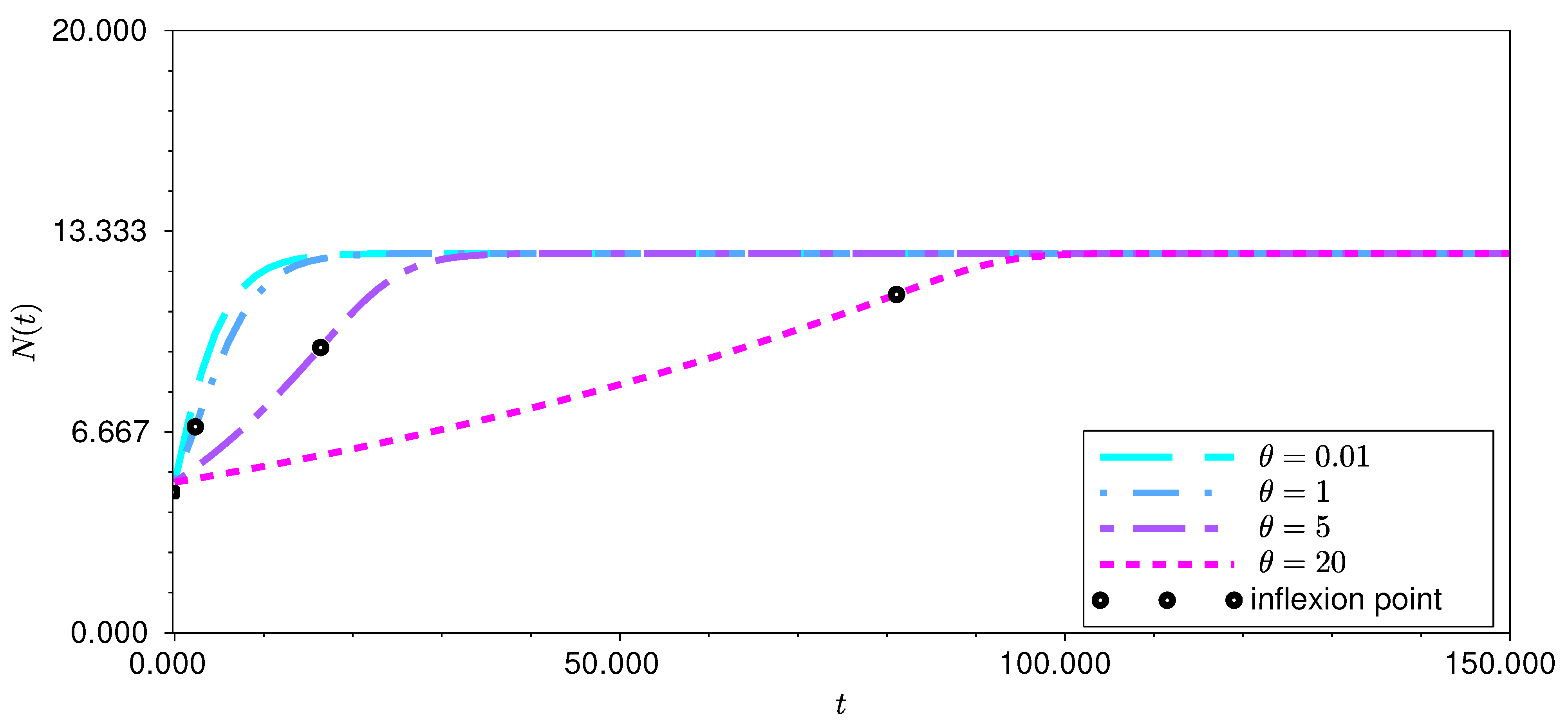
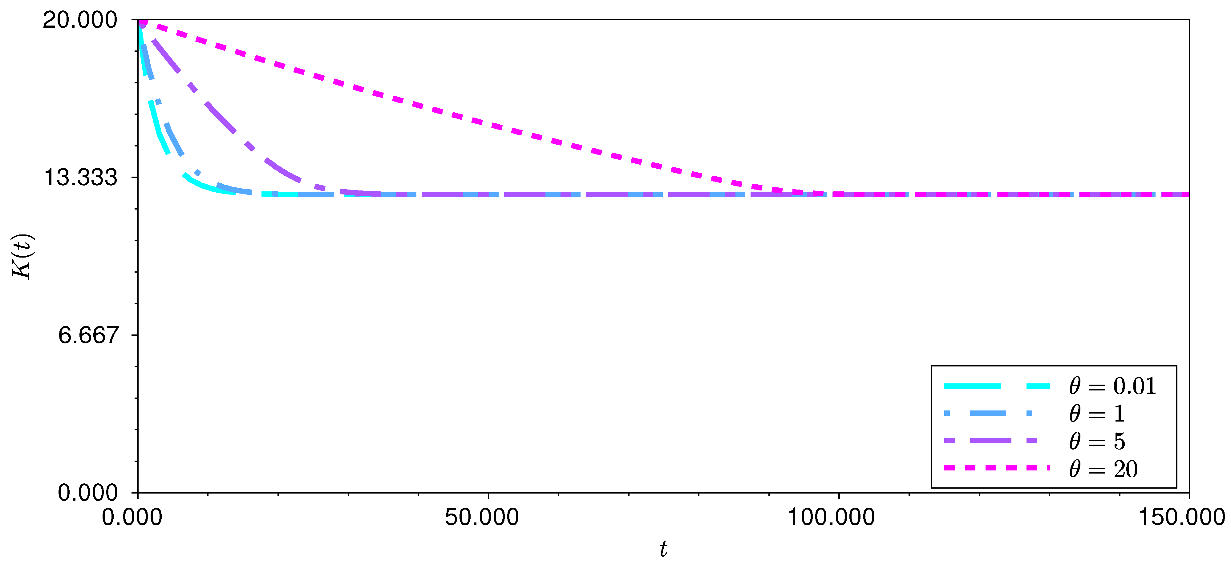
Example 1.

Let

$$\begin{array}{c}\hfill f(x,y)=\frac{a}{\theta }\left[1-{\left(\frac{x}{y}\right)}^{\theta }\right],g(x,y)=-\frac{b}{\theta }\left[1-{\left(\frac{x}{y}\right)}^{\theta }\right],\end{array}$$

(10)

where $a,b>0$ and $\theta \ge 0$. Then $g(x,y)=\alpha f(x,y)$, where $\alpha =-\frac{b}{a}<0$. Thus, (1) becomes

$$\frac{\mathrm{d}N}{\mathrm{d}t}=\frac{a}{\theta }N\left[1-{\left(\frac{N}{K}\right)}^{\theta }\right],\frac{\mathrm{d}K}{\mathrm{d}t}=-\frac{b}{\theta }K\left[1-{\left(\frac{N}{K}\right)}^{\theta }\right],N\left(0\right)=N_0,K\left(0\right)=K_0.$$

(11)

The ‘value’ when $\theta =0$ is meant to be understood as the limit when $\theta \to 0^{+}$; this is related to the Gompertz model in the case of a constant carrying capacity. The Thornley–France model (2) is a special case of (10) if we take $\theta =1$. From the first equation of (9), we obtain

$$t=\frac{\theta }{a}{\int }_{N_0}^{N\left(t\right)}\frac{1}{z[1-{\left(K_0{N}_0^{-\alpha }\right)}^{-\theta }{z}^{\theta (1-\alpha )}]}\mathrm{d}z=\frac{1}{a(1-\alpha )}{\int }_{{\left(K_0{N}_0^{-\alpha }\right)}^{-\theta }{N}_0^{\theta (1-\alpha )}}^{{\left(K_0{N}_0^{-\alpha }\right)}^{-\theta }{\left[N\left(t\right)\right]}^{\theta (1-\alpha )}}\frac{1}{u(1-u)}\mathrm{d}u.$$

(12)

Recall the formula

$$I\left(u\right)=\int \frac{1}{u(1-u)}\mathrm{d}u=log\left(\frac{u}{1-u}\right),0<u<1.$$

If $I\left(b_0\right)-I\left(a_0\right)=c_0$, where $0<a_0<b_0<1$ and $c_0>0$, then it is not difficult to show that

$$b_0=\frac{1}{1+\frac{1-a_0}{a_0}{\mathrm{e}}^{-c_0}}.$$

Taking $a_0={\left(K_0{N}_0^{-\alpha }\right)}^{-\theta }{N}_0^{\theta (1-\alpha )}={\left(K_0^{-1}{N}_0\right)}^{\theta }$, $b_0={\left(K_0{N}_0^{-\alpha }\right)}^{-\theta }{\left[N\left(t\right)\right]}^{\theta (1-\alpha )}$ and $c_0=a(1-\alpha )t$, we deduce that the exact solution of (11) is

$$\begin{array}{c}\hfill N\left(t\right)={\left[\frac{{\left(K_0{N}_0^{-\alpha }\right)}^{\theta }}{1+\frac{1-{\left(K_0^{-1}{N}_0\right)}^{\theta }}{{\left(K_0^{-1}{N}_0\right)}^{\theta }}{\mathrm{e}}^{-a(1-\alpha )t}}\right]}^{\frac{1}{\theta (1-\alpha )}},K\left(t\right)=K_0{N}_0^{-\alpha }{\left[N\left(t\right)\right]}^{\alpha }.\end{array}$$

(13)

As $a,b>0$ and $\alpha =-\frac{b}{a}<0$, we have from (13) that

$$N_{\infty }=\underset{t\to \infty }{lim}N\left(t\right)={\left(K_0{N}_0^{-\alpha }\right)}^{\frac{1}{1-\alpha }},K_{\infty }=\underset{t\to \infty }{lim}K\left(t\right)={\left(K_0{N}_0^{-\alpha }\right)}^{\frac{1}{1-\alpha }}.$$

This is consistent with the fact that $f(N_{\infty },K_{\infty })=g(N_{\infty },K_{\infty })=0$ in (11) yields that any equilibrium of (11), and there are infinitely many, lies on the curve $K_{\infty }=N_{\infty }$.

Let us now look at the inflexion points of N by studying the roots of $H\left(z\right)=0$ in (7). Straightforward calculations give

$$D_{1}f(x,y)=-\frac{a}{x}{\left(\frac{x}{y}\right)}^{\theta },D_{2}f(x,y)=\frac{a}{y}{\left(\frac{x}{y}\right)}^{\theta },x{F}^{\prime }\left(x\right)=\alpha F\left(x\right),$$

$$x{D}_{1}f(x,y)=-a+\theta f(x,y),y{D}_{2}f(x,y)=a-\theta f(x,y).$$

If we define

$$H_0(x,y)=f(x,y)+x{D}_{1}f(x,y)+\alpha y{D}_{2}f(x,y),$$

then $H\left(z\right)=0$ if and only if $H_0(z,F\left(z\right))=0$. However, $H_0(x,y)=[1+\theta (1-\alpha )]f(x,y)-a(1-\alpha )$, so that $H_0(z,F\left(z\right))=0$ if and only if

$$\frac{a}{\theta }\left[1-{\left(\frac{z}{F\left(z\right)}\right)}^{\theta }\right]=f(z,F\left(z\right))=\frac{a(1-\alpha )}{1+\theta (1-\alpha )}.$$

This is equivalent to

$${\left[\frac{1}{1+\theta (1-\alpha )}\right]}^{\frac{1}{\theta }}=\frac{z}{F\left(z\right)}=\frac{z}{K_0{N}_0^{-\alpha }{z}^{\alpha }}={\left(\frac{z}{K_{\infty }}\right)}^{1-\alpha },K_{\infty }={\left(K_0{N}_0^{-\alpha }\right)}^{\frac{1}{1-\alpha }}.$$

Thus $H\left(N^{*}\right)=0$ if and only if

$$N^{*}=K_{\infty }{\left[\frac{1}{1+\theta (1-\alpha )}\right]}^{\frac{1}{\theta (1-\alpha )}}.$$

(14)

Finally, we see from (8) that

$$\begin{array}{cc}\hfill t^{*}& =\frac{1}{a(1-\alpha )}\left[I{\left(\left(\frac{N^{*}}{K_{\infty }}\right)\right)}^{\theta (1-\alpha )})-I\left({\left(\frac{N_0}{K_{\infty }}\right)}^{\theta (1-\alpha )}\right)\right].\hfill \end{array}$$

(15)

As I is an increasing function of u, and assuming that $N_0<N^{*}$, it follows that $t^{*}>0$.

It was already noted that $\theta =1$ in (10) reduces to the Thornley–France model (2). Then, if $\theta =1$, (13) recovers the analytical solution found in Thornley et al. [15]. Equation (14) indicates where inflexion occurs as a fraction of the asymptotic carrying capacity, while (15) gives the time of inflexion (compare with (17) and (18), respectively, found in Thornley et al. [15] with an appropriate renaming of parameters).

On the other hand, when we let $\theta \to \infty$, then (14) shows that $\frac{N^{*}}{K_{\infty }}$ tends to unity so that, similar to the Thornley–France model when $\theta =1$, exponential growth is sustained for longer and the inflexion value $N^{*}$ moves closer to the asymptotic carrying capacity value $K_{\infty }$.

If $\theta >0$ and $\alpha =0$ (corresponding to $b=0$ in (10)), then $K\left(t\right)=K_0$ and (1) reduces to a single ODE

$$\frac{\mathrm{d}N}{\mathrm{d}t}=\frac{a}{\theta }N\left[1-{\left(\frac{N}{K_0}\right)}^{\theta }\right],$$

which is the θ-logistic model. In particular, if $\theta =1$ and $\alpha =0$ (i.e., the ‘ordinary’ logistic model), then (14) shows that the inflexion value is one-half of the asymptotic carrying capacity value, which is well known. If $\theta \to 0^{+}$, then we deduce from (14) that $\frac{N^{*}}{K_{\infty }}$ tends to $\frac{1}{\mathrm{e}}$ for any $\alpha =-\frac{b}{a}<0$. This is similar in behaviour to the case when $\alpha =0$ (i.e., $b=0$ in (10)), so that $K\left(t\right)=K_0$ and (1) recovers the Gompertz model

$$\frac{\mathrm{d}N}{\mathrm{d}t}=aNlog\left(\frac{K_0}{N}\right).$$

Thus $\frac{N^{*}}{K_{\infty }}$ tends to $\frac{1}{\mathrm{e}}$ as $\theta \to 0^{+}$ even for the variable carrying capacity system (11).

Here we include some results of numerical simulations of (11) (equivalently, (13)). Let $a=0.2$, $b=0.1$, $N_0=5$ and $K_0=20$. Take four different values of $\theta =0.01,1,5,20$ to see and compare the population dynamics, as shown in Figure 1, as well as the carrying capacity behaviour in Figure 2.

As can be seen in both figures, the larger the value of θ, the longer it takes for the population and carrying capacity to reach equilibrium.

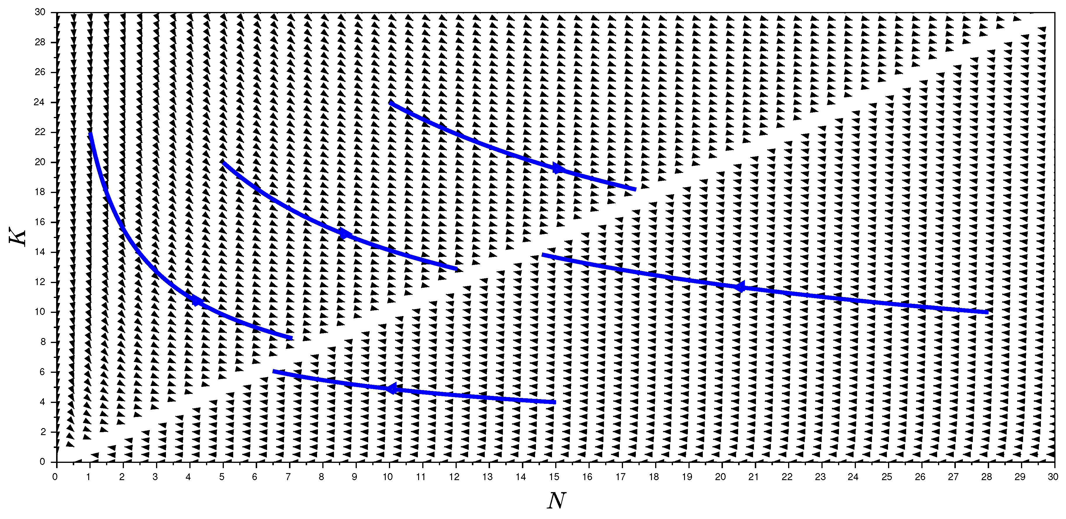
Figure 3 ($\theta =0.01$) and Figure 4 ($\theta =1.2$) depict some trajectories in the $NK$-plane and illustrate that the carrying capacity experiences a decline as the population grows larger. This is a consequence of the proportionality of the per capita growth rates with a negative proportionality constant. Moreover, when the initial conditions are varied, the trajectories approach the equilibrium line $K_{\infty }=N_{\infty }$. This behaviour is typical for other values of θ as well.

2.4. Second Class of Analytically Tractable Models: f and g Are Homogeneous Functions

Suppose that f and g in (1) are homogeneous functions, i.e.,

$$f(\lambda x,\lambda y)=\lambda f(x,y),g(\lambda x,\lambda y)=\lambda g(x,y)\mathrm{for}\mathrm{every}\lambda >0.$$

Let $v=\frac{y}{x}$ in (4), so that $g(x,y)=g(x,xv)=xg(1,v)$ and $f(x,y)=f(x,xv)=xf(1,v)$. Then (4) is transformed into the separable ODE

$$x\frac{\mathrm{d}v}{\mathrm{d}x}=v\frac{g(1,v)-f(1,v)}{f(1,v)},$$

whose general solution is

$$\mathsf{\Phi }\left(v\right)=\mathsf{\Phi }\left(\frac{y}{x}\right)=log\left(x\right)+log\left(C\right),\mathsf{\Phi }\left(v\right)=\int \frac{f(1,v)}{v\left[g\right(1,v)-f(1,v\left)\right]}\mathrm{d}v,$$

(16)

where $C>0$ is an arbitrary constant of integration. Hence, assuming that $\mathsf{\Phi }$ is invertible, we deduce that the solution of (4) is

$$y=F\left(x\right)=x{\mathsf{\Phi }}^{-1}(log\left(Cx\right)),log\left(C\right)=\mathsf{\Phi }\left(\frac{K_0}{N_0}\right)-log\left(N_0\right).$$

(17)

Next, we determine G. From (5), we see that

$$G\left(x\right)={\int }_{N_0}^x\frac{1}{zf(z,z{\mathsf{\Phi }}^{-1}(log\left(Cz\right)))}\mathrm{d}z.$$

(18)

Finally, (6) implies that the exact solution of (1) in the case when both f and g are homogeneous functions is

$${\int }_{N_0}^{N\left(t\right)}\frac{1}{zf(z,z{\mathsf{\Phi }}^{-1}(log\left(Cz\right)))}\mathrm{d}z=t,K\left(t\right)=N\left(t\right){\mathsf{\Phi }}^{-1}(log\left(CN\left(t\right)\right)).$$

(19)

Example 2.

Let

$$f(x,y)=a\left(1-\frac{x}{y}\right),g(x,y)=a-\frac{cx}{y},$$

where $0<a<c$, so that (1) becomes

$$\frac{\mathrm{d}N}{\mathrm{d}t}=aN\left(1-\frac{N}{K}\right),\frac{\mathrm{d}K}{\mathrm{d}t}=K\left(a-\frac{cN}{K}\right),N\left(0\right)=N_0,K\left(0\right)=K_0;$$

(20)

compare with model (3) proposed by Safuan et al. [10]. Observe that f and g are homogeneous functions but are not proportional since $a<c$. Then (16) gives

$$\mathsf{\Phi }\left(v\right)=\frac{a}{a-c}[v-log\left(v\right)],\mathsf{\Phi }\left(\frac{y}{x}\right)=\frac{a}{a-c}\left[\frac{y}{x}-log\left(\frac{y}{x}\right)\right]=log\left(Cx\right)$$

(21)

and, therefore,

$$\left(\frac{c}{a}-1\right)log\left(C{N}_0\right)=log\left(\frac{K_0}{N_0}\right)-\frac{K_0}{N_0}\mathrm{or}{\left(C{N}_0\right)}^{\frac{c}{a}-1}=\frac{K_0}{N_0}{\mathrm{e}}^{-\frac{K_0}{N_0}}.$$

(22)

The second equation in (21) can be rewritten as

$$-\frac{y}{x}{\mathrm{e}}^{-\frac{y}{x}}=-exp\left(-\frac{a-c}{a}log\left(Cx\right)\right)=-{\left(Cx\right)}^{\frac{c}{a}-1}.$$

(23)

Let us recall some properties of the Lambert W-function. Suppose that $u,z\in \mathbb{R}$. Then $z=W\left(u\right)$ satisfies the equation $z{\mathrm{e}}^z=u$ if $u\ge -\frac{1}{\mathrm{e}}$. Furthermore, $W\left(u\right)<0$ for $-\frac{1}{\mathrm{e}}\le u<0$ and

$$W^{\prime }\left(u\right)=\frac{W\left(u\right)}{u[1+W(u\left)\right]},u\ne -\frac{1}{\mathrm{e}},0.$$

(24)

Identifying

$$z=-\frac{y}{x},u=-{\left(Cx\right)}^{\frac{c}{a}-1},$$

and assuming that $0<x\le \frac{1}{C}{\mathrm{e}}^{\frac{a}{a-c}}$ so that $u\ge -\frac{1}{\mathrm{e}}$, we obtain from (23) that

$$y=F\left(x\right)=-xW(-{\left(Cx\right)}^{\frac{c}{a}-1}).$$

We see that $F\left(x\right)>0$ since the W-function is negative here because $-\frac{1}{\mathrm{e}}\le u<0$. Following a similar argument, we deduce from (21) that

$${\mathsf{\Phi }}^{-1}\left(z\right)=-W(-{\mathrm{e}}^{-\frac{a-c}{a}z}),{\mathsf{\Phi }}^{-1}(log\left(Cz\right))=-W(-{\left(Cz\right)}^{\frac{c}{a}-1}).$$

Therefore, (18) yields

$$\begin{array}{cc}\hfill G\left(x\right)& =\frac{1}{a}{\int }_{N_0}^x\frac{W(-{\left(Cz\right)}^{\frac{c}{a}-1})}{z[1+W(-{\left(Cz\right)}^{\frac{c}{a}-1})]}\mathrm{d}z=\frac{1}{c-a}{\int }_{-{\left(C{N}_0\right)}^{\frac{c}{a}-1}}^{-{\left(Cx\right)}^{\frac{c}{a}-1}}\frac{W\left(u\right)}{u[1+W(u\left)\right]}\mathrm{d}u\hfill \\ \hfill & =\frac{1}{c-a}[W(-{\left(Cx\right)}^{\frac{c}{a}-1})-W(-{\left(C{N}_0\right)}^{\frac{c}{a}-1})],\hfill \end{array}$$

where we used (24) in the last step. Equation (22) gives

$$W(-{\left(C{N}_0\right)}^{\frac{c}{a}-1})=W\left(-\frac{K_0}{N_0}{\mathrm{e}}^{-\frac{K_0}{N_0}}\right)=-\frac{K_0}{N_0}$$

since $z=W\left(u\right)=W\left(z{\mathrm{e}}^z\right)$ if $u=z{\mathrm{e}}^z$. Hence the exact solution of (20) from (19) is

$$\begin{array}{c}\hfill W(-{\left[CN\left(t\right)\right]}^{\frac{c}{a}-1})=-\frac{K_0}{N_0}+(c-a)t,K\left(t\right)=-N\left(t\right)W(-{\left[CN\left(t\right)\right]}^{\frac{c}{a}-1}).\end{array}$$

(25)

Example 3.

Suppose that

$$\begin{array}{c}\hfill f(x,y)=alog\left(\frac{y}{x}\right),g(x,y)=alog\left(\frac{y}{x}\right)+b,\end{array}$$

where $a,b>0$. Therefore, (1) becomes

$$\frac{\mathrm{d}N}{\mathrm{d}t}=aNlog\left(\frac{K}{N}\right),\frac{\mathrm{d}K}{\mathrm{d}t}=K\left[alog\left(\frac{K}{N}\right)+b\right],N\left(0\right)=N_0,K\left(0\right)=K_0.$$

(26)

We see that f and g are homogeneous functions but are not proportional as $b>0$. Then (16) implies that

$$\mathsf{\Phi }\left(v\right)=\frac{a}{2b}{[log\left(v\right)]}^2,\mathsf{\Phi }\left(\frac{y}{x}\right)=\frac{a}{2b}{\left[log\left(\frac{y}{x}\right)\right]}^2=log\left(Cx\right)$$

and

$$log\left(C\right)=\frac{a}{2b}{\left[log\left(\frac{K_0}{N_0}\right)\right]}^2-log\left(N_0\right),{[log\left(C{N}_0\right)]}^{\frac{1}{2}}={\left(\frac{a}{2b}\right)}^{\frac{1}{2}}log\left(\frac{K_0}{N_0}\right).$$

(27)

Since

$${\mathsf{\Phi }}^{-1}\left(v\right)=exp\left({\left(\frac{2b}{a}v\right)}^{\frac{1}{2}}\right),{\mathsf{\Phi }}^{-1}(log\left(Cv\right))=exp\left({\left[\frac{2b}{a}log\left(Cv\right)\right]}^{\frac{1}{2}}\right),$$

Equation (17) yields

$$y=F\left(x\right)=xexp\left({\left[\frac{2b}{a}log\left(Cx\right)\right]}^{\frac{1}{2}}\right).$$

Furthermore,

$$f(z,z{\mathsf{\Phi }}^{-1}(log\left(Cz\right)))=a{\left[\frac{2b}{a}log\left(Cz\right)\right]}^{\frac{1}{2}}={\left(2ab\right)}^{\frac{1}{2}}{[log\left(Cz\right)]}^{\frac{1}{2}}$$

and from (18), we obtain

$$\begin{array}{cc}\hfill G\left(x\right)& =\frac{1}{{\left(2ab\right)}^{\frac{1}{2}}}{\int }_{N_0}^x\frac{1}{z{[log\left(Cz\right)]}^{\frac{1}{2}}}\mathrm{d}z=\frac{1}{{\left(2ab\right)}^{\frac{1}{2}}}{\int }_{log\left(C{N}_0\right)}^{log\left(Cx\right)}{u}^{-\frac{1}{2}}\mathrm{d}u\hfill \\ \hfill & ={\left(\frac{2}{ab}\right)}^{\frac{1}{2}}{[log\left(Cx\right)]}^{\frac{1}{2}}-{\left(\frac{2}{ab}\right)}^{\frac{1}{2}}{[log\left(C{N}_0\right)]}^{\frac{1}{2}}.\hfill \end{array}$$

Substituting into (19) gives ${[log\left(CN\left(t\right)\right)]}^{\frac{1}{2}}={[log\left(C{N}_0\right)]}^{\frac{1}{2}}+{\left(\frac{ab}{2}\right)}^{\frac{1}{2}}t$, which simplifies to

$$\begin{array}{c}\hfill log\left(CN\left(t\right)\right)=log\left(C{N}_0\right)+atlog\left(\frac{K_0}{N_0}\right)+\frac{ab}{2}{t}^2\end{array}$$

using (27). Thus,

$$N\left(t\right)=N_0{\left(\frac{K_0}{N_0}\right)}^{at}{\mathrm{e}}^{\frac{ab}{2}{t}^2}.$$

Moreover, (19) also implies that

$$K\left(t\right)=N\left(t\right)exp\left({\left[\frac{2b}{a}log\left(CN\left(t\right)\right)\right]}^{\frac{1}{2}}\right),$$

so that

$$\begin{array}{cc}\hfill log\left(K\right(t\left)\right)& =log\left(N\left(t\right)\right)+{\left[\frac{2b}{a}log\left(CN\left(t\right)\right)\right]}^{\frac{1}{2}}\hfill \\ \hfill & =log\left(N\left(t\right)\right)+{\left(\frac{2b}{a}\right)}^{\frac{1}{2}}{[log\left(C{N}_0\right)]}^{\frac{1}{2}}+{\left(\frac{2b}{a}\right)}^{\frac{1}{2}}{\left(\frac{ab}{2}\right)}^{\frac{1}{2}}t\hfill \\ \hfill & =log\left(N\left(t\right)\right)+log\left(\frac{K_0}{N_0}\right)+bt.\hfill \end{array}$$

Hence

$$K\left(t\right)=\frac{K_0}{N_0}{\mathrm{e}}^{bt}N\left(t\right)=\frac{K_0}{N_0}{\mathrm{e}}^{bt}{N}_0{\left(\frac{K_0}{N_0}\right)}^{at}{\mathrm{e}}^{\frac{ab}{2}{t}^2}=K_0{\left(\frac{K_0}{N_0}\right)}^{at}{\mathrm{e}}^{\frac{ab}{2}{t}^2+bt}.$$

Thus, the exact solution of (26) is

$$\begin{array}{c}\hfill N\left(t\right)=N_0{\left(\frac{K_0}{N_0}\right)}^{at}{\mathrm{e}}^{\frac{ab}{2}{t}^2},K\left(t\right)=K_0{\left(\frac{K_0}{N_0}\right)}^{at}{\mathrm{e}}^{\frac{ab}{2}{t}^2+bt}.\end{array}$$

(28)

2.5. Third Class of Analytically Tractable Models: f and g Determine an Exact ODE

Assume that f and g are such that

$$\frac{\partial }{\partial x}\left[xf(x,y)\right]+\frac{\partial }{\partial y}\left[yg(x,y)\right]=f(x,y)+x{D}_{1}f(x,y)+g(x,y)+y{D}_{2}g(x,y)=0.$$

(29)

This implies that (4) is an exact ODE whose general solution is $\mathsf{\Psi }(x,y)=C=\mathsf{\Psi }(N_0,K_0)$, where C is an arbitrary constant of integration and

$$D_1\mathsf{\Psi }(x,y)=-yg(x,y),D_2\mathsf{\Psi }(x,y)=xf(x,y).$$

(30)

Then

$$\mathsf{\Psi }(x,y)=-\int yg(x,y)\mathrm{d}x+Q\left(y\right)=\int xf(x,y)\mathrm{d}y+P\left(x\right),$$

(31)

where $P=P\left(x\right)$ and $Q=Q\left(y\right)$ are arbitrary functions of integration. Differentiating $\mathsf{\Psi }$ in (31) with respect to y and using the second equation in (30) and then (29), we get

$$Q\left(y\right)=\int \left[xf(x,y)-\int f(x,y)\mathrm{d}x-\int x{D}_{1}f(x,y)\mathrm{d}x\right]\mathrm{d}y.$$

(32)

An analogous calculation yields

$$P\left(x\right)=\int \left[-yg(x,y)-\int f(x,y)\mathrm{d}y-\int x{D}_{1}f(x,y)\mathrm{d}y\right]\mathrm{d}x.$$

(33)

Assuming that $\mathsf{\Psi }(x,y)=C=\mathsf{\Psi }(N_0,K_0)$ can be solved for $y=F\left(x\right)$, then we have from (5) and the second equation in (30) that

$$G\left(x\right)={\int }_{N_0}^x\frac{1}{zf(z,F(z\left)\right)}\mathrm{d}z={\int }_{N_0}^x\frac{1}{D_2\mathsf{\Psi }(z,F\left(z\right))}\mathrm{d}z.$$

(34)

Therefore, (6) expresses the exact solution of (1) as

$${\int }_{N_0}^{N\left(t\right)}\frac{1}{D_2\mathsf{\Psi }(z,F\left(z\right))}\mathrm{d}z=t,K\left(t\right)=F\left(N\left(t\right)\right).$$

(35)

Looking at condition (29) more closely, we conclude that

$$yg(x,y)=-\int f(x,y)\mathrm{d}y-\int x{D}_{1}f(x,y)\mathrm{d}y+R\left(x\right)$$

(36)

for some arbitrary function $R=R\left(x\right)$. Hence the exactness condition (29) necessarily implies the above form for g. Thus from (31) and (36), we have

$$\begin{array}{cc}\hfill \mathsf{\Psi }(x,y)& =\int \left[\int f(x,y)\mathrm{d}y+x\int D_{1}f(x,y)\mathrm{d}y-R\left(x\right)\right]\mathrm{d}x\hfill \\ \hfill & +\int \left[xf(x,y)-\int f(x,y)\mathrm{d}x-\int x{D}_{1}f(x,y)\mathrm{d}x\right]\mathrm{d}y\hfill \\ \hfill & =\int xf(x,y)\mathrm{d}y-\int R\left(x\right)\mathrm{d}x.\hfill \end{array}$$

This simplified form for $\mathsf{\Psi }$ is then substituted into the first equation in (35).

Example 4.

Let $a>0$. If

$$f(x,y)=a\left(1-\frac{x}{y}\right)=a-ax{y}^{-1},D_{1}f(x,y)=-a{y}^{-1},$$

then (36) evaluates to $yg(x,y)=-ay+2axlog\left(y\right)$, taking $R\left(x\right)=0$ for simplicity. Therefore, (1) becomes

$$\frac{\mathrm{d}N}{\mathrm{d}t}=aN\left(1-\frac{N}{K}\right),\frac{\mathrm{d}K}{\mathrm{d}t}=-aK+2aNlog\left(K\right),N\left(0\right)=N_0,K\left(0\right)=K_0.$$

(37)

We have

$$\mathsf{\Psi }(x,y)=\int x(a-ax{y}^{-1})\mathrm{d}y=ax[y-xlog\left(y\right)],$$

where $C=\mathsf{\Psi }(N_0,K_0)=a{N}_0[K_0-N_{0}log\left(K_0\right)]$. The equation $\mathsf{\Psi }(x,y)=C$ gives

$$log\left(y\right)-\frac{y}{x}=-\frac{C}{a}{x}^{-2},-\frac{y}{x}{\mathrm{e}}^{-\frac{y}{x}}=-x^{-1}exp\left(-\frac{C}{a}{x}^{-2}\right).$$

Hence, as in Example 2,

$$y=F\left(x\right)=-xW\left(-x^{-1}exp\left(-\frac{C}{a}{x}^{-2}\right)\right)\mathrm{if}-x^{-1}exp\left(-\frac{C}{a}{x}^{-2}\right)\ge -\frac{1}{\mathrm{e}}.$$

Then

$$D_2\mathsf{\Psi }(x,y)=ax-a{x}^2{y}^{-1},D_2\mathsf{\Psi }(z,F\left(z\right))=az\left[1-\frac{z}{F\left(z\right)}\right]$$

and

$$1-\frac{z}{F\left(z\right)}=\frac{1+W(-z^{-1}exp(-\frac{C}{a}{z}^{-2})}{W(-z^{-1}exp(-\frac{C}{a}{z}^{-2})}.$$

From (34) we obtain

$$G\left(x\right)=\frac{1}{a}{\int }_{N_0}^x\frac{W(-z^{-1}exp(-\frac{C}{a}{z}^{-2})}{z[1+W(-z^{-1}exp(-\frac{C}{a}{z}^{-2})]}\mathrm{d}z,$$

which cannot be further evaluated analytically (unlike in Example 2). The exact solution of (37) using (35) is

$$\begin{array}{c}\hfill {\int }_{N_0}^{N\left(t\right)}\frac{W(-z^{-1}exp(-\frac{C}{a}{z}^{-2})}{z[1+W(-z^{-1}exp(-\frac{C}{a}{z}^{-2})]}\mathrm{d}z=at,\\ \hfill K\left(t\right)=-N\left(t\right)W\left(-{\left[N\left(t\right)\right]}^{-1}exp\left(-\frac{C}{a}{\left[N\left(t\right)\right]}^{-2}\right)\right).\end{array}$$

(38)

3. Concluding Remarks

In this article, we proposed population models with variable carrying capacities modelled by a coupled system (1) of two nonlinear ODEs and found their analytical solutions. While it was clear that the assumptions $D_{1}f(x,y)<0$ and $D_{2}f(x,y)>0$ are reasonable since they describe the behaviour of the population per capita growth rate, we showed through several explicit examples that corresponding assumptions for $D_{1}g(x,y)$ and $D_{2}g(x,y)$ that describe the carrying capacity per capita growth rate are not obvious and may be model dependent. One possible reason for this is that carrying capacity is not directly observable, unlike the population size.

If the per capita growth rates are proportional, as in Example 1, then in addition to the analytical solution, we also found a criterion for the occurrence of inflexion in the population profile as a fraction of the asymptotic carrying capacity. This criterion does not apply to the models in Examples 2 and 3 since they do not have a nontrivial equilibrium. However, it should apply for the model in Example 4 with a nontrivial equilibrium $(N_{\infty },K_{\infty })=({\mathrm{e}}^{-\frac{1}{2}},{\mathrm{e}}^{-\frac{1}{2}})$. Further classes of analytically tractable models of the form (1), not necessarily in the context of population growth with variable carrying capacity, can, of course, be found by considering analytically tractable cases of (4) following the idea in Rodrigo [25].

Future work would involve a more careful investigation of the assumptions for the carrying capacity per capita growth rate. While this article focused on the analytical aspects of population models with variable carrying capacities, fitting the models to actual population data is the next important step. The estimation of parameters in the models can be undertaken by adapting the arguments in Zulkarnaen & Rodrigo [12], Holder & Rodrigo [13]. Parameter estimation using an integration-based technique in population models with variable carrying capacities that depend on food availability is the subject of an article by the authors that is currently under review [26]. Another research direction is the modelling of interacting population species where the carrying capacities are not fixed anymore but may depend on time and/or space. Results for predator–prey models have been obtained in Al-Moqbali et al. [18], Albano et al. [23], although spatio-temporal models (e.g., chemotaxis [27]) can also be considered. Travelling waves are an important class of biologically relevant solutions for spatio-temporal models described by partial differential equations. A travelling wave coordinate transformation leads to a system of higher dimensional ODEs, for which analytically tractable models can potentially be identified using the techniques in the current article.